Decision-Making Model under Risk Assessment Based on Entropy

Abstract

Decision-making under risk assessment involves dealing with the matter of uncertainty, especially in projects such as tunnel construction. Risk control should include not only measures to reduce the possible consequence of incident, but also exploration measures (information collecting measures) to reduce the uncertainty of the incident. The classical risk assessment model in engineering is $R=P\times C$ which only takes account of the assessment and decision-making of possible consequences. It cannot provide theoretical guidance for taking exploration measures. The paper presents an advanced methodology to assess the effectiveness of exploration measures in decision-making. The methodology classifies risk into two attributes: hazard (expected value) and uncertainty (entropy). On this basis, a generalized model of decision-making under risk assessment is proposed. This model extends the use of the classical assessment model to a more general case. The reason for taking exploration measures and assessment of such measures’ effectiveness could be explained well by this developed model. This model can also serve as a descriptive model for many risk problems and provide a decision-making basis for a variety of risk types. Moreover, the assessment process and calculation method are applied with some case studies.

1. Introduction

Risk assessment and management are widely applied to large engineering projects with increasing frequency [1]. Several methods for assessing and managing risk have been established and supported by approved standards and guidelines [2]. Risk analysis may be qualitative, semi-quantitative or quantitative. The risk analysis and evaluation tools that are commonly used in geotechnical engineering and tunneling, include fault tree analysis (FTA), event tree analysis (ETA), bowtie diagrams, multi-risk analysis, probabilistic risk analysis (PRA) [3,4,5,6,7], analytical hierarchy process (AHP) [8], bayesian networks (BN) [9,10,11], fuzzy logic and other artificial intelligence (AI) methods [12,13]. Recently, new approaches and methods have been developed in hazard assessment and risk analysis. Vicari et al. [14] provided an excellent means for assessing the hazard posed by ongoing effusive eruptions. For tunneling, attribute synthetic evaluation [15] and fuzzy mathematics [16,17,18] were used to assess the risk of water inrush in karst tunnels. Abdolreza [18] proposed a new methodology based on fuzzy logic for tunneling risk assessment. Choi et al. [12] presented a risk assessment methodology for underground construction projects. In terms of the methodology, an uncertainty model based on the fuzzy concept was built to evaluate risk. The fuzzy-based uncertainty model was designed to consider the uncertainty range that represents the degree of uncertainty involved in both (i) probabilistic parameter estimates and (ii) subjective judgments. Geographic Information System (GIS) technology was also used to dynamically predict the water inrush in the process of tunnel construction [19]. Fouladgar et al. [20] used the TOPSIS method to solve multi-criteria decision-making problems in tunneling projects. The above studies laid a solid foundation for the development of risk assessment and provided the basis of decision-making.

Currently, decision-making under risk is based on the level of risk which is assessed by the previous risk analysis step. The level of risk is defined as the “magnitude of a risk or combination of risks, expressed in terms of the combination of consequences and their likelihood.” In general, risk can be described as a 2D combination of probability and consequence [21]. In other words, risk is a type of expected value. In addition, the decision-making model under risk is the expected utility model which was developed by von Neumann and Morgenstern [22]. However, uncertainty-related risk is more than just the expected value. Some researchers clarified the meaning of risk in other ways. Amundrud and Aven [23] classified risk into two types: risk = (C, P) and risk = (C, U), where C is the consequence of the activities studied, and U refers to uncertainty. He and Huang [24] proposed the risk attribute theory, which classified risk into four attributes: expected value, expectation and variance, entropy, and relative maximum absolute value.

Hence, decision-making under risk assessment is one of the fundamental issues and has been a heated issue in recent years [25,26,27]. Cornell and Dillon [28] explored the respective roles of risk and decision analysis in decision support. Many studies have been conducted to extend the classical decision-making model under risk [29,30,31,32]. Pedrycz and Chen [33] stated that decision-making is inherently interactive. The facets of interactivity and the iterative way in which decisions are formed gave rise to granular computing. Meanwhile, a special issue regarding granular computing [34,35,36,37,38,39,40,41,42,43,44,45,46,47,48,49,50,51] was published to systematically introduce granular computing and its application. It is worthy of future research to apply granular computing techniques to solve risk assessment problems. On the other hand, it should be noted that risk is highly related to uncertainty. The influence of uncertainty should a concerned of the decision-making under risk. The concept of entropy is used to quantify uncertainty [52,53,54]. Entropy has been found applications in many fields, such as statics, physics, communication, ecology, etc. [55]. Some researchers did creative and meaningful work to apply entropy to decision-making. Yang and Qiu [29] extended the classical decision model under risk to a more general case and proposed an expected utility-entropy (EU-E) measure of risk and a decision-making model. The model mainly reflected an individual’s intuitive attitude towards risk. Recently, Yang and Qiu [56] continue to improve the EU-E measure of risk and the decision model and proposed the normalized EU-E decision model. Additionally, an entropy-based approach is being applied in other fields [57,58].

The classical risk assessment in engineering is R = P × C. This model mainly takes account of the possible consequence of incident which consists of the probability and consequence of an incident. However, many risk questions are highly related to the uncertainty of the risk incident itself. The less information we know about the risk incident, the more uncertainty there exists in the risk incident and the less effective are the measures taken. When confronting deep uncertainty with insufficient information, one may first want to examine the effect of collecting information prior to making a decision.

The objective of risk assessment is to provide a basis for risk control measures, which should include pre-control measures to reduce the possible consequence of risk and exploration measures to reduce uncertainty. For example, the advanced geological forecast is widely used in tunnel construction. However, the question that arises here is what kind of measure should a decision-maker choose and why. The classical model only takes account of the assessment and decision-making of possible consequences. It cannot provide theoretical guidance for taking exploration measures. The initial aim of our recommended model is to solve this problem.

The paper presents a methodology to provide theoretical guidance for exploration measures (information collecting measures). The methodology classifies risk into two attributes: expected value and entropy. Expected value denotes the possible consequence of the risk incident and entropy denotes the uncertainty involved in the incident. Based on this methodology, a new decision-making model under risk is proposed. This model extends the use of the classical assessment model to a more general case. Also, this model can serve as a descriptive model for many risk problems and provide a decision-making basis for variety of risk types.

2. Classification of Risk Problem

The processes and mechanisms of risk occurrence are discussed before analyzing the risk assessment model. The past, present, and future of our natural world are dominated by the laws of science, which are found or remain to be found. In our natural world, random or uncertain things are poorly understood. To some extent, the uncertainty in probability theory stems from our limited knowledge and cognition of our world. In this view, coin tossing is taken as an example. The final probability of each side of a coin is 0.5. However, if we know the initial state of the toss and the mechanics law dominating the movement of the coin, then we can know which side will appear. Thus, the probability is finite in this case.

If we apply the above thought to risk analysis, then a risk incident can be denoted by the following: the occurrence of incident A is determined by mechanisms and influencing factors that led to the occurrence of the incident. If the mechanisms and influencing factors are fully understood and clear, then the occurrence of the incident is certain. In this case, no risk exists in the incident.

We apply this thought to a general case. The occurrence of incident A is determined by the formula $y=f(x_1,x_2,x_3,\dots ,x_n)$, where $(x_1,x_2,x_3,\dots ,x_n)$ are the influencing factors leading to the occurrence of the incident, and $f$ is the operator of the formula. When $y\le 0$, incident A does not occur. When $y>0$, incident A happens. If $(x_1,x_2,x_3,\dots ,x_n)$ are certain and f is clear or known, then y is certain. In other words, risk is absent. This scenario can be expressed by the following formula:

$$P(\mathrm{A}|x_1,x_2,x_3,\dots ,x_n)=0 \text{or} 1$$

(1)

The occurrence of the incident is uncertain when one or some values of $x_1,x_2,x_3,\dots ,x_n$ are uncertain or the mechanism is unclear. This case can be denoted as a risk incident, which is classified into two categories.

Case 1.

One, or some, values of $x_1,x_2,x_3,\dots ,x_n$ are uncertain. For example, the value of $x_1$ is in an interval [a, b]. In this case, $y$ is uncertain and there is a certain probability distribution. The probability distribution of $y$ is related to the probability distribution of $x_1$ . The occurrence probability of risk incident A can be expressed by the following formula:

$$P(\mathrm{A}|x_1,x_2,x_3,\dots ,x_n)=P(y>0)$$

(2)

Case 2.

The form of the index set is transformed to $(x_1,x_2,x_3,\dots ,x_m,x_{m+1},x_{m+2},\dots ,x_n)$, where $(x_1,x_2,x_3,\dots ,x_m)$ represents the index set in which the influencing factors are clear and can be obtained, and $(x_{m+1},x_{m+2},\dots ,x_n)$ represents the influencing factors that are obscure and uncertain or whose values are hard to obtain. In consideration of the above unclear elements, an uncertainty exists in risk incident A. The state of incident A can be judged by the known influencing factors. Thus, we can obtain the following formula:

$$P(\mathrm{A}|x_1,x_2,x_3,\dots ,x_m)=[0, 1]$$

(3)

For risk assessment, known experience/knowledge or statistical analysis of historical data can be used to obtain the formula between $(x_1,x_2,x_3,\dots ,x_m)$ and the occurrence probability of the incident as follows:

$$P(\mathrm{A}|x_1,x_2,x_3,\dots ,x_m)=f(x_1,x_2,x_3,\dots ,x_m)$$

(4)

where the result is a probability constant when $x_1,x_2,x_3,\dots ,x_m$ are certain or a probability distribution when one or some values of $x_1,x_2,x_3,\dots ,x_m$ are uncertain.

In general, risk problems can be divided into the two above-mentioned cases.

3. Discussion of the Risk Assessment Model

3.1. Applicability of the R = P × C Classical Model

Classical risk assessment in engineering is R = P × C. P represents the probability of an incident while C represents the consequence of the incident. This model mainly takes account of the hazard state of the incident, which consists of the probability and consequence of the hazard. However, many risk questions are highly related to the uncertainty of risk incidents. The less information we know about a risk incident, the more uncertainty there exists in the risk incident and the less effectiveness are the measures taken. The measures taken to reduce risk may not be so feasible under this circumstance. The final objective of risk assessment is to implement decision-making for risk disposition. Risk control should include not only measures to reduce the hazard of the incident, but also the exploration of measures to reduce the uncertainty of the risk incident.

For example, the risk pre-control measures for water inrush in a tunnel risk assessment include the following measures:

• The line of extra-long tunnel is designed to be of a gable slope for drainage.
• Comprehensive advanced geological forecasting, which includes conventional geological methods, comprehensive advanced geophysical exploration, and horizontal borehole advanced forecasting (five holes of every main tunnel section, and three holes of every parallel guide-pit tunnel), is applied in high-risk active fault regions and fault fracture zones.
• Comprehensive advanced geological forecasting, which includes conventional geological methods, comprehensive advanced geophysical exploration, and horizontal borehole advanced forecasting (three holes for every main tunnel section, and one hole for every parallel guide-pit tunnel), is applied in the syncline and anticline of the soluble rock region.
• According to the surrounding rock and water enrichment situation, a parallel driftway between the main tunnel and water enrichment area is excavated to reduce the water inrush hazard of the groundwater for the main tunnel.

Among the above measures, the first and fourth measures are aimed to reduce the possible hazard of water inrush. Meanwhile, the second and third measures are exploration measures which are aimed at gaining more information about the geological conditions. These measures all take a lot of time and cost a significant amount of money. Thus, it is necessary to evaluate what kind of measures to take before making a decision. However, the current classical risk assessment model cannot provide a feasible basis according to this circumstance.

We take Case 1 for further illustration.

Risk incident A is assumed to be influenced by elements $x_1,x_2$ and the formula is $y=\frac{x_1}{x_2}-1$, where if $y\le 0$ incident A does not happen, and if $y>0$ incident A does happen.

For the value of $x_1,x_2$, the more accurate the information obtained, the more money spent.

Table 1. Risk factors’ value and risk value (R = P × C).

	Risk Factors		Risk Value
	${\mathit{x}}_{\mathbf{1}}$	${\mathit{x}}_{\mathbf{2}}$	Probability	Outcome	Risk Value
Before taking exploration measures	(0, 2)	1	0.5	C	0.5C
After taking exploration measures	(0.9, 1.4)	1	0.8	C	0.8C

shows the risk factors’ value and risk value after taking exploration measures whose cost is T.

In Table 1, the value of $x_1$ is in an interval. There is no more specific information about $x_1$. According to the maximum entropy theory, $x_1$ obeys an even distribution. From Table 1, we can obtain the decreased value $\Delta R$ after taking exploration measures:

$$\Delta R=0.5C-0.8C=-0.3C$$

From the above formula, the risk value increases, rather than decreases, according to the typical risk assessment model. However, in essence, it decreases the risk after taking exploration measures which narrows the interval of $x_1$. The current risk assessment model cannot give a clear explanation for this question as the model does not take account of uncertainty.

3.2. Applicability Discussion of the Expected Utility-Entropy Model

Shannon [59], the founder of information theory, measured the objective uncertainty of the state of nature by entropy in his landmark paper. Entropy is used to represent the uncertainty degree of a system. After defining and calculating entropy, Yang and Qiu [29] proposed a new model based on the expected utility and entropy for decision-making under risk. In this model, the measure of risk when taking action is defined as:

$$R(\mathrm{a})=\lambda H_a(\theta )-(1-\lambda )\frac{E[\mu (X(a,\theta ))]}{\text{max}\{E[\mu (X(a,\theta ))]\}}$$

(5)

where risk is characterized by the combination of expectation and entropy, and entropy is used to represent the uncertainty of the outcome/income.

Fischer and Kleine [60] questioned this model and they argued that the new model violates basic normative principles and does not agree with the observed patterns of actual human behavior and risk perception. They took a concrete example to provide a clear interpretation. The example is as follows:

A lottery of the shape (10, 0.1; 10.01, 0.1; 9.98, 0.1; 9.95, 0.1; 10.02, 0.1; 10.05, 0.1; 9.97, 0.1; 10.03, 0.1; 9.99, 0.1; 10.04, 0.1) has a high entropy of 2.3, although the outcome is close to 10 in each possible state. However, the lottery (8, 0.5; 11, 0.5) has an entropy of 0.69. The expected values of the two lotteries are 10.014 and 9.5, respectively. According to expected utility and entropy theory, the second lottery would be more advisable than the first one. Not only does the former have a higher expected value, it also seems to be far less “risky”.

On the basis of the discussion in Section 3.1, the assessment model must consider the measure of uncertainty. However, the example in Section 3.2 easily demonstrates the limitation of expected utility and entropy.

The role of entropy in the field of risk decision theory could not be denied just because of the question of the expected utility and entropy model. The application of this model is based on certain preconditions. The examples of Fischer and Kleine [60] have a common feature, i.e., the casualness of the range. The formula of entropy indicates that entropy is highly related to the number of values of the range. The expected utility and entropy model is unsuitable when the number of values of the range is unlimited and the range interval is unstable. However, this new thought provides a meaningful idea on the uncertainty under risk.

For example, the outcome interval is (1, 2, 3, 4), and the corresponding probability interval is $(p_1,p_2,p_3,p_4)$. The following two choices are available:

• a: $p_1,p_2,p_3,p_4=(0.25, 0.25, 0.25, 0.25)$
• b: $p_1,p_2,p_3,p_4=(0, 0.5, 0.5, 0)$

The two choices have the same range, on the basis of the calculation, E(a) = E(b) = 2.5; H(a) = 1.38; H(b) = 0.69. Obviously, b would be the choice.

In risk assessment, the range is generally stable and complete with a definitive assessment object. Thus, entropy can be used to represent uncertainty as a part of the risk assessment model. Risk consists of two parts: hazard and entropy. Hazard is characterized by $P\times C$ (in the presence of many outcomes, the formula can be ${\sum }_{i=1}^n{P}_i{C}_i$). Entropy H represents uncertainty. If we take ${\sum }_{i=1}^n{P}_i{C}_i$ as an expected value, then expected utility and entropy can provide a reference for the risk assessment model. However, this model cannot simply be applied in risk assessment.

• The expected utility and entropy model is different from the typical risk assessment model in application. The former is for the choice between different schemes. The objective of risk assessment is to provide a basis for risk disposition.
• Entropy represents the uncertainty of different outcomes in the expected utility and entropy model. However, the first step in risk assessment is hazard classification. Risk control measures correspond with risk levels. Thus, entropy in risk assessment should be used to represent the uncertainty of risk levels. In addition, the calculation of entropy should be different from that of the expected utility and entropy model.
• The value of entropy is not related to the expected value in the expected utility and entropy model. However, in this way, risk assessment does not make sense for the following reasons:

  (a)

  When the hazard is relatively small, people would not take measures to reduce the uncertainty no matter how large the uncertainty is. For example, people must choose between two ways ahead. No useful information for decision-making currently exists. People who make a wrong choice will suffer great losses. Under this circumstance, people would pay the price to obtain useful information. However, if the price of making a wrong choice is acceptable, people would not take measures to reduce the uncertainty of this state. In the expected utility and entropy model, high entropy means high risk. It does not make sense under this circumstance.

  (b)

  When the hazard is large, people would pay the price to obtain further information on uncertainty reduction. The more serious the consequences are when people make a wrong choice, the more people would spend on obtaining information.

Based on the discussion above, we propose a new risk assessment model founded on entropy under risk.

4. Our Recommend Approach

4.1. Entropy-Hazard Risk Assessment Model

A risk assessment model should consist of three elements: probability P, consequence C, and entropy H. Probability and consequence represent the hazard of risk, which is denoted by R₁. Entropy represents the uncertainty of risk, which is denoted by R₂. Risk assessment of the incident is conducted by analyzing the above three elements.

The objective of risk assessment is to provide a basis for risk control measures, which include pre-control measures to reduce the possible hazard of risk and exploration measures to reduce uncertainty. For example, advanced geological forecasting is widely used in tunnel construction. However, the question that arises here is what kind of measure should a decision-maker choose, and why. The initial objective of our recommended model is to solve this problem.

The classical risk assessment model is based on pre-control measures. Risk is classified into different levels that correspond to different pre-control measures. As shown in

Table 2. Classification of the risk level.

Frequency	Consequence
	Disastrous	Severe	Serious	Considerable	Insignificant
Very likely	Unacceptable	Unacceptable	Unacceptable	Unwanted	Unwanted
Likely	Unacceptable	Unacceptable	Unacceptable	Unwanted	Acceptable
Occasional	Unacceptable	Unwanted	Unwanted	Acceptable	Acceptable
Unlikely	Unwanted	Unwanted	Acceptable	Acceptable	Negligible
Very unlikely	Unwanted	Acceptable	Acceptable	Negligible	Negligible

, the International Tunneling Association classifies risk into four levels: “unacceptable”, “unwanted”, “acceptable”, and “negligible” [61]. For the risk level “unacceptable”, measures must be taken regardless of the cost to reduce risk. The cost should also be in accordance with the profit that the decrease of risk makes.

On the basis of the above discussion, reducing entropy should be one part of risk control. The risk assessment model considering uncertainty should obey the following principles:

• When the hazard is relatively large, people would pay the price to reduce the uncertainty for risk control.
• No matter how large the uncertainty is, people would not take measures to reduce uncertainty when the hazard is small.
• If the hazard and uncertainty can be reduced to the same degree at the same cost, people would prefer choosing to reduce the hazard. For example, we assume that the hazard value of one incident is R₁ and the uncertainty value of that is R₂. When taking measures respectively, but at the same cost T, the hazard and uncertainty are reduced by 100%. People choose measures that reduce the hazard because risk is absent when the hazard value decreases to 0 regardless of the size of the uncertainty. By contrast, a risk still exists even when the entropy decreases to 0.

Risk assessment involving uncertainty can also be represented in economic terms. The economic terms involve two costs. One is the cost $T_H$ that the measures need to reduce uncertainty, and the other is the tolerance cost $T_H^{\prime }$ decision-makers accept when taking measures to reduce uncertainty. Hence, making a decision by comparing the two costs is suitable.

• When $T_H>T_H^{\prime }$, measures should not be taken;
• When $T_H<T_H^{\prime }$, measures can be taken.

The next step is to obtain the tolerance cost $T_H^{\prime }$.

According to the first and second principles above, the tolerance cost $T_H^{\prime }$ and hazard value have a direct ratio, which is expressed below:

$T_H^{\prime }=\alpha R_1$, where $\alpha$ is an undetermined coefficient, and $\alpha >0$.

Let $H^{\prime }$ and H be the entropy values after and before taking measures to reduce uncertainty, respectively. Then, the decreasing proportion would be $\frac{H-H^{\prime }}{H}$. According to the third principle, the tolerance cost should not be larger than the product of the decreasing proportion and hazard, as shown in Equation (6):

$$T_H^{\prime }<\frac{H-H^{\prime }}{H}{R}_1$$

(6)

According to formula (6) and $T_H^{\prime }=\alpha R_1$, the final formula of $T_H^{\prime }$ is represented below:

$$T_H^{\prime }=\alpha (\frac{H-H^{\prime }}{H})R_1$$

(7)

where $0<\alpha <1$, which represents the willingness of people to take measures to reduce uncertainty. The smaller $\alpha$ is, the less willing people are to pay the price to reduce uncertainty.

4.2. Calculation Method of Entropy

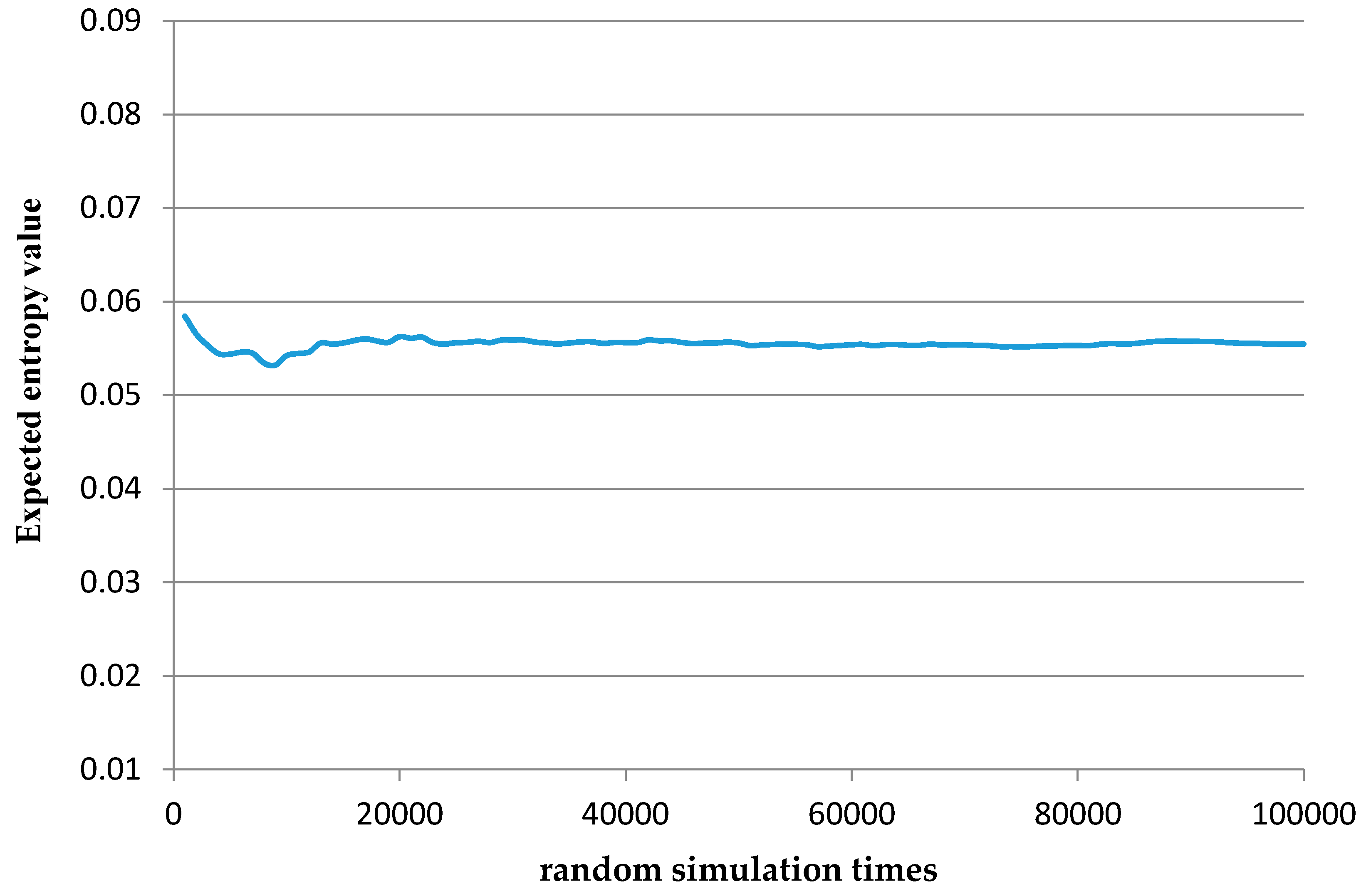
4.2.1. Calculation of the Entropy Value

Many uncertainty factors exist in risk assessment. Here, a question arises: which factor’s entropy should be taken as one part of the risk assessment model? We conduct the analysis on the two cases given in Section 2. The uncertainty analysis of the two cases is shown in

Table 3. Uncertainty analysis of the risk incident.

Case 1	Index Type	Influencing Factors	Risk
			Risk Incident	Occurrence Probability	Consequence	Risk Level
	Range	$(x_1,x_2,x_3,\dots ,x_n)$	$P(y>0),P(y\le 0)$	$P(y>0)$	C	$(R_1^1,R_1^2,R_1^3,R_1^4)$
	Entropy Value	>0	0~−ln(0.5)	0	0	0
Case 2	Index Type	Influencing Factors	Risk
			Risk Incident	Occurrence Probability	Consequence	Risk Level
	Range	$(x_1,x_2,x_3,\dots ,x_n)$	$P(y>0),P(y\le 0)$	$P(y>0)$	C	$(R_1^1,R_1^2,R_1^3,R_1^4)$
	Entropy Value	>0	>0	0	0	0~ln(0.25)

It should be noted that risk level is assumed to be classified into four grades, $(R_1^1,R_1^2,R_1^3,R_1^4)$, where $R_1^i$ represents the hazard component and $R_1$ belongs to grade i.

.

For Case 1, factors with uncertainty are risk-influencing factors and risk incidents. The former represents the uncertainty of risk-influencing factors, and the latter means that uncertainty exists in the occurrence of the risk incident.

Let H(X) be the entropy value of risk-influencing factors and H(A) be entropy value of risk incident A. Thus:

$$H(X)=f[H(x_1),H(x_2),H(x_3),\dots ,H(x_n)]$$

(8)

where $H(x_i)$ is the entropy value of factor i.

$$H(A)=-P(y>0)lnP(y>0)-P(y\le 0)lnP(y\le 0)$$

(9)

For Case 2, factors with uncertainty are risk-influencing factors, the risk incident, the occurrence probability, and the risk level. The meanings of the risk-influencing factors and risk incident are explained in Case 1. The uncertainty of the occurrence probability means that the occurrence probability is uncertain but obeys some probability distributions. Thus, the uncertainty of occurrence probability leads to the uncertainty of the risk level.

For Case 2, the entropy value formula of the risk-influencing factors and risk incident is the same as that for Case 1.

For the risk occurrence probability, if the occurrence probability obeys a discrete distribution, then H(P) can be denoted as follows:

$$H(P)=-{\displaystyle \sum _{i=1}^n}P(P_i)lnP(P_i)$$

(10)

If H(P) obeys a continuous distribution, then H(P) can be expressed as:

$$H(P)=\int f(P)lnf(P)dp$$

(11)

The entropy of the risk level is expressed as follows:

$$H(R_1)=-{\displaystyle \sum _{i=1}^4}P(R_1^i)lnP(R_1^i)$$

(12)

where $P(R_1^i)$ means the probability of R₁ belonging to grade i.

The above discussion indicates that uncertainty has four types, namely H(X), H(A), H(P), and H($R_1$). However, the type of uncertainty that can represent the second component $R_2$ of risk remains to be discussed.

Case 1 has only two choices: $R_2=H(X)$ or $R_2=H(A)$. $H(A)$ is definitely 0 when $H(X)$ is reduced to 0, but $H(X)$ is not definitely 0 when $H(A)$ is 0. For decision-makers, the occurrence of a risk incident is certain when $H(A)$ is 0. Thus, reducing $H(X)$ to 0 is unnecessary.

In the example in Section 3.1, $H(X)$ is large and $H(A)$ is 0 when the range of x₁ is [2, 10]. However, under this circumstance, decision-makers can definitely know that the incident will occur. Thus, reducing $H(X)$ is not needed, and $H(A)$ is taken as the value of R₂.

Case 2 has four choices: $R_2=H(X)$, $R_2=H(A)$, $R_2=H(P)$, or $R_2=H(R_1)$. When $H(X)$ is reduced to 0, $H(A)$ is not 0, and $H(P)$ and $H(R_1)$ are 0. $H(A)$ is not 0 because the uncertainty of the risk incident could not be reduced in Case 2. Under this circumstance, $H(P)$ is 0. $H(R_1)$ is also 0 when $H(P)$ is 0. However, $H(P)$ may be not 0 when $H(R_1)$ is 0. If $H(R_1)$ is 0, then decision-makers can definitely know which risk level the incident belongs to. Thus, reducing $H(P)$ to 0 is not needed.

For example, if the occurrence probability of risk obeys the even distribution (0.3, 0.8) and the distribution of the risk level is (1, 0, 0, 0), then decision-makers are certain that the risk belongs to $R_1^1$. Even if measures are taken to reduce the entropy of the occurrence probability, the final risk level will not change. Thus, we take H(R₁) to represent R₂ in Case 2.

4.2.2. Calculation Method of $H^{\prime }$

As shown in Equation (7), the entropy value after taking measures is required to obtain $T_H^{\prime }$. According to Section 4.2.1, the entropy value means $H(A)$ or $H(R_1)$. In general, the precision of one or some factors can be predicted to be reduced to a certain range after taking measures. However, knowing the exact range is difficult. For example, if the precision of x₁ is predicted to be 0.2 after taking measures, then the value of x₁ is in the interval of [a, a + 0.2]. If we assume that the initial range of x₁ is [0, 2], then the range of a is [0, 1.8]. The uncertainty of a leads to the uncertainty of y. Hence, determining the value of entropy $H(A)$ is difficult. However, the probability distribution of $H(A)$ can be obtained by the probability distribution of a and the formula between y and x₁. $E[H(A)]$, the expected value of $H(A)$, can also be obtained through the probability distribution of $H(A)$. Taking the expected entropy value as $H^{\prime }$ for entropy is reasonable after taking measures, such as the predictive entropy. Thus, $H^{\prime }$ can be expressed as follows:

$$H^{\prime }=\{\begin{array}{c}E[H(A)], \text{Case} 1\\ E[H(R_1)], \text{Case} 2\end{array}$$

(13)

On the basis of the probability distribution of risk factors, data simulation can be performed using the Monte Carlo method to obtain the expected entropy value. According to the theorem of large numbers, the expected entropy value converges along with the increasing number of simulation times. Then, the final convergence value is the expected entropy value.

As shown in Figure 1, a certain variation of the expected entropy value exists when the number of simulation times is less than 30,000. Along with the increasing number of simulation times, the expected entropy value gradually converges to a stable value of 0.055.

5. Assessment Process and Case Study

Risk assessment should obey the principle that the uncertainty should initially be reduced, followed by the hazard. The specific risk assessment process is shown in Figure 2.

In addition, an algorithm is presented to describe the proposed approach in detail.

• Step 1: Analyze risk incidents and obtain information about risk incidents, including influencing factors $x_1,x_2,x_3,\cdots ,x_n$ and their values.
• Step 2: Enter the initial parameters: C, $T_{H,i}$ (the cost of ith exploration measures) and $x_1,x_2,x_3,\cdots ,x_n$.
• Step 3: Determine the risk category to which the incident belongs and calculate P, H.
  If it belongs to Case 1, the probability P is calculated using formula (2), and H is calculated using formula (9);
  If it belongs to Case 2, the probability P is calculated using formula (3), and H is calculated using formula (12).
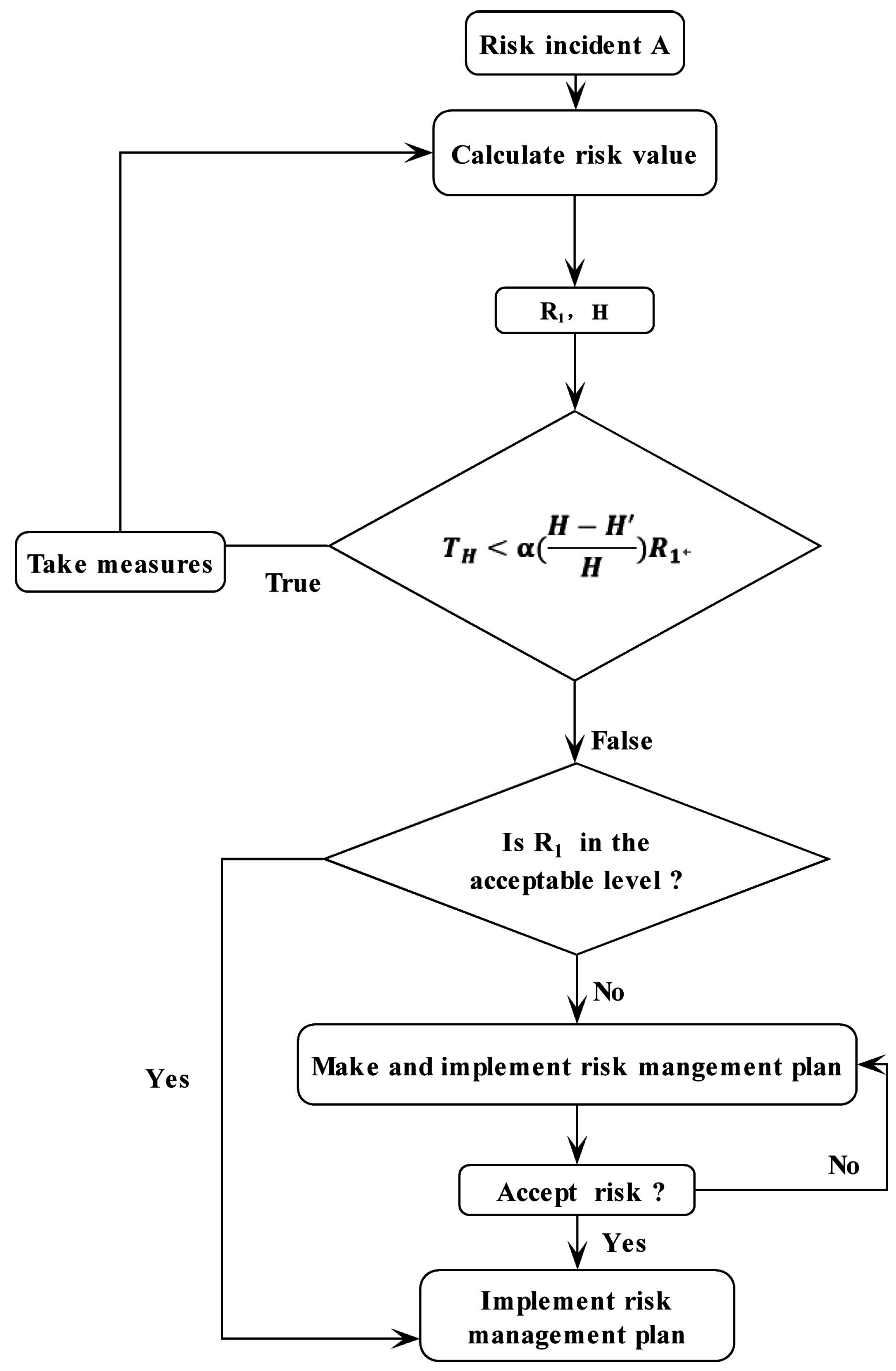
• Step 4: Calculate $H^{\prime }$ using formula (13) and calculate $T_{H,i}^{\prime }$ using formula (7). If $T_{H,i}$ < $T_{H,i}^{\prime }$ (the tolerance cost of i-th exploration measures), continue to step 5; otherwise, skip to step 6.
• Step 5: After taking measures, update initial parameters: $x_1,x_2,x_3,\cdots ,x_n$, C, $T_{H,i}$ and $\alpha$. Calculate the updated probability P using formula (2) or (3).
• Step 6: Determine whether to take risk control measures according to the value $R_1$ and acceptance criteria. In addition, implement the next risk management plan. A simple example is made to provide a specific explanation.

The occurrence of risk incident A is related to several factors. Among the factors, $x_1,x_2,x_3$ are currently known. According to the statistical analysis of historical data, the fitting formula between the occurrence probability of incident A and the influencing factors is $P(A)=0.1x_1+0.07x_2^2+0.09x_2+0.05x_3$, where $x_1,x_2,x_3\in (0, 1)$.

The risk level and acceptable criterion are given in

Table 4. Risk level of risk incident A.

Risk Level	Scope of Risk Component R1	Risk-Acceptable Criterion
$R_1^1$	>106	Unacceptable
$R_1^2$	105~106	Unwanted
$R_1^3$	5 × 103~105	Acceptable
$R_1^4$	<5 × 103	Negligible

. The risk value is represented by the form of expense.

According to experienced experts, the occurrence of incident A will cause a loss of 5 × 10⁶. The value ranges of $x_1,x_2,x_3$ are $x_1\in (0.005,0.03)$, $x_2\in (0,0.3)$, and $x_3\in (0.05,0.2)$, respectively. The occurrence probability of risk P and H(R₁) can be calculated using the Mote Carlo method. As the probability is uncertain, P is replaced with the expected probability. Then, we can obtain P = 0.0236 and H(R₁) = 0.6754. The probabilities of second-grade and third-grade risk levels are 0.6 and 0.4, respectively.

According to the analysis of experts, further exploration measures of $x_1,x_2,x_3$ are given. The expense and expected effect are shown in

Table 5. Expense and expected effect of exploration measures.

Number of Measure	Target Factor	Expense	Expected Precision Range
1	$x_1$	13,000	0.005
2	$x_2$	20,000	0.05
3	$x_2$	10,000	0.1
4	$x_3$	30,000	0.01

.

On the basis of Equation (7), $H^{\prime }$ and $T_H^{\prime }$ are calculated (here, we assume α = 1/5) as follows:

• Measure 1: $H^{\prime }$ = 0.6743, $T_H^{\prime }$ =38.44
• Measure 2: $H^{\prime }$ = 0.1842, $T_H^{\prime }$ = 17,164
• Measure 3: $H^{\prime }$ = 0.3173, $T_H^{\prime }$ = 12,502
• Measure 4: $H^{\prime }$ = 0.6667, $T_H^{\prime }$ = 303

Compared with the real expense, only the expense of Measure 3 is lower than the tolerance cost. Thus, Measure 3 would be the final choice. After taking Measure 3, the value range of $x_2$ is (0.15, 0.25). The risk value is recalculated to obtain P = 0.0289 and H(R₁) = 0.0358. The entropy is rather small, and the risk level is in the second-grade risk level, the probability of which is 0.9942.

At this time, further uncertainty reduction is not needed. According to the risk-acceptable criterion in Table 4, the second-grade risk level belongs to the level “unacceptable”. Thus, measures must be taken to reduce the hazard. However, the cost of measures must be larger than the profit the measures make. Then, the problem can be solved by the classical risk decision-making model.

6. Conclusions and Discussion

How to handle deep uncertainties is a main foundational issue in risk assessment and risk management. The question of how to define and measure uncertainty is particularly critical in decision-making under risk. Uncertainty is essentially the absence of information, which may or may not be obtainable. Classical decision-making under risk deals with choices of different risk control measures without regard for exploration measures, such as advanced geological forecasting in tunnel construction. Prior to making decisions, people may first want to examine the effect of collecting further information.

The objective of our proposed approach is to provide a basis for risk control measures, which should include pre-control measures to reduce the possible consequence of risk and exploration measures to reduce uncertainty. The paper presents a methodology to provide theoretical guidance for exploration measures (information collecting measures). The methodology classifies risk into two attributes: expected value and entropy. Expected value denotes the possible consequence of the risk incident and entropy denotes the uncertainty involved in the incident. Based on this methodology, a new decision-making model under risk is proposed. Finally, the following conclusions are drawn:

• The occurrence of risk incidents is assumed to be determined by a certain formula and influencing factors. On the basis of this assumption, risk incidents are classified into two categories.
• Uncertainty is taken as a part of the risk assessment model, and it is expressed by entropy. Importantly, the calculation formula of entropy is given under different circumstances.
• Entropy may be used to represent uncertainty under risk. With regard to the interrelation between hazard and uncertainty, a new risk assessment model based on entropy is developed.
• Decision strategies for reducing uncertainty are based on the value of information. Specifically, the comparison between reducing hazard and reducing uncertainty is expressed in terms of cost. If the value of collecting information, namely reducing uncertainty, is larger than that of reducing hazard, then the measures taken to reduce uncertainty are tolerable and available.
• Risk assessment under uncertainty involves a decision to reduce uncertainty or reduce hazard. The general assessment process of our model is based on the criterion that uncertainty is first reduced, followed by the hazard.

This paper confirms the feasibility of the new model by introducing examples. However, the model remains to be demonstrated in practical and universal decision-making problems under risk. By theory, the proposed model can serve as a decision-making basis for selecting measures that should be taken for certain problems. This model can serve as a descriptive model for many risk problems. Furthermore, this model might provide risk analysts with different ideas on the issue of risk management.

References

1. Einstein, H.H. Risk and risk analysis in rock engineering. Tunn. Undergr. Space Technol. 1996, 11, 141–155. [Google Scholar] [CrossRef]
2. Aven, T.; Zio, E. Foundational issues in risk assessment and risk management. Risk Anal. 2014, 34, 1164–1172. [Google Scholar] [CrossRef] [PubMed]
3. Brown, E.T. Risk assessment and management in underground rock engineering—An overview. J. Rock Mech. Geotech. Eng. 2012, 4, 193–204. [Google Scholar] [CrossRef]
4. Baecher, G.B.; Christian, J.T. Reliability and Statistics in Geotechnical Engineering; Wiley: New York, NY, USA, 2003. [Google Scholar]
5. Fenton, G.A.; Griffiths, D.V. Risk Assessment in Geotechnical Engineering; Wiley: New York, NY, USA, 2008. [Google Scholar]
6. Honjo, Y.; Suzuki, M.; Hara, T.; Zhang, F. (Eds.) Geotechnical Risk and Safety; CRC Press: Leiden, The Netherlands, 2009.
7. Juang, C.H.; Phoon, K.K.; Puppala, A.J.; Green, R.A.; Fenton, G.A. (Eds.) GeoRisk 2011: Geotechnical Risk Assessment and Management; ASCE: Reston, VA, USA, 2011.
8. Taroun, A.; Yang, J.B. Dempster–Shafer theory of evidence: Potential usage for decision making and risk analysis in construction project management. Built Hum. Environ. Rev. 2011, 4 (Suppl. 1), 155–166. [Google Scholar]
9. Jensen, F.V.; Nielsen, T.D. Bayesian Networks and Decision Graphs, 2nd ed.; Springer: New York, NY, USA, 2007. [Google Scholar]
10. Sousa, R.L.; Einstein, H.H. Risk analysis during tunnel construction using Bayesian networks: Porto metro case study. Tunn. Undergr. Space Technol. 2012, 27, 86–100. [Google Scholar] [CrossRef]
11. Sousa, R.L. Risk Analysis for Tunneling Projects. Ph.D. Thesis, Massachusetts Institute of Technology, Cambridge, MA, USA, 2010. [Google Scholar]
12. Choi, H.H.; Cho, H.N.; Seo, J.W. Risk assessment methodology for underground construction projects. J. Constr. Eng. Manag. 2004, 130, 258–272. [Google Scholar] [CrossRef]
13. Zhou, H.B.; Zhang, H. Risk assessment methodology for a deep foundation pit construction project in Shanghai, China. J. Constr. Eng. Manag. 2011, 137, 1185–1194. [Google Scholar] [CrossRef]
14. Vicari, A.; Ciraudo, A.; Del Negro, C.; Herault, A.; Fortuna, L. Lava flow simulations using discharge rates from thermal infrared satellite imagery during the 2006 Etna Eruption. Nat. Hazards 2009, 50, 539–550. [Google Scholar] [CrossRef]
15. Li, S.C.; Zhou, Z.Q.; Li, L.P.; Xu, Z.H.; Zhang, Q.Q.; Shi, S.S. Risk assessment of water inrush in karst tunnels based on attribute synthetic evaluation system. Tunn. Undergr. Space Technol. 2013, 38, 50–58. [Google Scholar] [CrossRef]
16. Li, L.; Lei, T.; Li, S.; Zhang, Q.; Xu, Z.; Shi, S.; Zhou, Z. Risk assessment of water inrush in karst tunnels and software development. Arab. J. Geosci. 2015, 8, 1843–1854. [Google Scholar] [CrossRef]
17. Ge, Y.H.; Li, S.C.; Zhang, Q.S.; Lu, W. Risk analysis of water inrush into karst tunnel using fuzzy comprehensive evaluation method. In Proceedings of the International Workshop on Intelligent Systems and Applications (ISA 2009), Wuhan, China, 23–24 May 2009; pp. 1–4.
18. Yazdani-Chamzini, A. Proposing a new methodology based on fuzzy logic for tunnelling risk assessment. J. Civ. Eng. Manag. 2014, 20, 82–94. [Google Scholar] [CrossRef]
19. Li, X.; Li, Y. Research on risk assessment system for water inrush in the karst tunnel construction based on GIS: case study on the diversion tunnel groups of the Jinping II Hydropower Station. Tunn. Undergr. Space Technol. 2014, 40, 182–191. [Google Scholar] [CrossRef]
20. Fouladgar, M.M.; Yazdani-Chamzini, A.; Zavadskas, E.K. Risk evaluation of tunneling projects. Arch. Civ. Mech. Eng. 2012, 12, 1–12. [Google Scholar] [CrossRef]
21. Aven, T. A semi-quantitative approach to risk analysis, as an Alternative to QRAs. Reliab. Eng. Syst. Saf. 2008, 93, 790–797. [Google Scholar] [CrossRef]
22. Von Neumann, J.; Morgenstern, O. The Theory of Games and Economic Behavior; Princeton University Press: Princeton, NJ, USA, 1944. [Google Scholar]
23. Amundrud, Ø.; Aven, T. On how to understand and acknowledge risk. Reliab. Eng. Syst. Saf. 2015, 142, 42–47. [Google Scholar] [CrossRef]
24. He, Y.; Huang, R.H. Risk attributes theory: Decision making under risk. Eur. J. Oper. Res. 2008, 186, 243–260. [Google Scholar] [CrossRef]
25. Tom, S.M.; Fox, C.R.; Trepel, C.; Poldrack, R.A. The neural basis of loss aversion in decision-making under risk. Science 2007, 315, 515–518. [Google Scholar] [CrossRef] [PubMed]
26. Karagoz, S.; Aydin, N.; Isikli, E. Decision Making in Solid Waste Management under Fuzzy Environment. In Intelligence Systems in Environmental Management: Theory and Applications; Springer: Cham, Switzerland, 2017. [Google Scholar]
27. Kahneman, D.; Tversky, A. Prospect theory: An analysis of decision under risk. Econometrica 1979, 47, 263–291. [Google Scholar] [CrossRef]
28. Paté-Cornell, M.E.; Dillon, R.L. The respective roles of risk and decision analysis in decision support. Decis. Anal. 2006, 3, 220–232. [Google Scholar] [CrossRef]
29. Yang, J.; Qiu, W. A measure of risk and a decision-making model based on expected utility and entropy. Eur. J. Oper. Res. 2005, 164, 792–799. [Google Scholar] [CrossRef]
30. Bell, D.E. Risk, return, and utility. Manag. Sci. 1995, 41, 23–30. [Google Scholar] [CrossRef]
31. Jia, J.; Dyer, J.S.; Butler, J.C. Measures of perceived risk. Manag. Sci. 1999, 45, 519–532. [Google Scholar] [CrossRef]
32. Dyer, J.S.; Jia, J. Relative risk-value models. Eur. J. Oper. Res. 1997, 103, 170–185. [Google Scholar] [CrossRef]
33. Pedrycz, W.; Chen, S.M. Granular Computing and Decision-Making: Interactive and Iterative Approaches; Springer: Heidelberg, Germany, 2015. [Google Scholar]
34. Peters, G.; Weber, R. DCC: A framework for dynamic granular clustering. Granul. Comput. 2016, 1, 1–11. [Google Scholar] [CrossRef]
35. Livi, L.; Sadeghian, A. Granular computing, computational intelligence, and the analysis of non-geometric input spaces. Granul. Comput. 2016, 1, 13–20. [Google Scholar] [CrossRef]
36. Xu, Z.; Wang, H. Managing multi-granularity linguistic information in qualitative group decision making: An overview. Granul. Comput. 2016, 1, 21–35. [Google Scholar] [CrossRef]
37. Antonelli, M.; Ducange, P.; Lazzerini, B.; Marcelloni, F. Multi-objective evolutionary design of granular rule-based classifiers. Granul. Comput. 2016, 1, 37–58. [Google Scholar] [CrossRef]
38. Mendel, J.M. A comparison of three approaches for estimating (synthesizing) an interval type-2 fuzzy set model of a linguistic term for computing with words. Granul. Comput. 2016, 1, 59–69. [Google Scholar] [CrossRef]
39. Lingras, P.; Haider, F.; Triff, M. Granular meta-clustering based on hierarchical, network, and temporal connections. Granul. Comput. 2016, 1, 71–92. [Google Scholar] [CrossRef]
40. Skowron, A.; Jankowski, A.; Dutta, S. Interactive granular computing. Granul. Comput. 2016, 1, 95–113. [Google Scholar] [CrossRef]
41. Dubois, D.; Prade, H. Bridging gaps between several forms of granular computing. Granul. Comput. 2016, 1, 115–126. [Google Scholar] [CrossRef]
42. Loia, V.; D’Aniello, G.; Gaeta, A.; Orciuoli, F. Enforcing situation awareness with granular computing: A systematic overview and new perspectives. Granul. Comput. 2016, 1, 127–143. [Google Scholar] [CrossRef]
43. Yao, Y. A triarchic theory of granular computing. Granul. Comput. 2016, 1, 145–157. [Google Scholar] [CrossRef]
44. Ciucci, D. Orthopairs and granular computing. Granul. Comput. 2016, 1, 159–170. [Google Scholar] [CrossRef]
45. Kreinovich, V. Solving equations (and systems of equations) under uncertainty: How different practical problems lead to different mathematical and computational formulations. Granul. Comput. 2016, 1, 171–179. [Google Scholar] [CrossRef]
46. Wilke, G.; Portmann, E. Granular computing as a basis of human-data interaction: A cognitive cities use case. Granul. Comput. 2016, 1, 181–197. [Google Scholar] [CrossRef]
47. Min, F.; Xu, J. Semi-greedy heuristics for feature selection with test cost constraints. Granul. Comput. 2016, 1, 199–211. [Google Scholar] [CrossRef]
48. Maciel, L.; Ballini, R.; Gomide, F. Evolving granular analytics for interval time series forecasting. Granul. Comput. 2016, 1, 213–224. [Google Scholar] [CrossRef]
49. Apolloni, B.; Bassis, S.; Rota, J.; Galliani, G.L.; Gioia, M.; Ferrari, L. A neuro fuzzy algorithm for learning from complex granules. Granul. Comput. 2016, 1, 225–246. [Google Scholar] [CrossRef]
50. Song, M.; Wang, Y. A study of granular computing in the agenda of growth of artificial neural networks. Granul. Comput. 2016, 1, 247–257. [Google Scholar] [CrossRef]
51. Liu, H.; Gegov, A.; Cocea, M. Rule-based systems: A granular computing perspective. Granul. Comput. 2016, 1, 259–274. [Google Scholar] [CrossRef] [Green Version]
52. Cover, T.M.; Thomas, J.A. Elements of Information Theory; Wiley: Hoboken, NJ, USA, 2012. [Google Scholar]
53. Renyi, A. On measures of entropy and information. In Proceedings of the Fourth Berkeley Symposium on Mathematical Statistics and Probability, Berkeley, CA, USA, 20 June–30 July 1961; pp. 547–561.
54. Tsallis, C. Possible generalization of Boltzmann-Gibbs statistics. J. Stat. Phys. 1988, 52, 479–487. [Google Scholar] [CrossRef]
55. Chen, B.; Wang, J.; Zhao, H.; Principe, J. Insights into Entropy as a Measure of Multivariate Variability. Entropy 2016, 18, 196. [Google Scholar] [CrossRef]
56. Yang, J.; Qiu, W. Normalized Expected Utility-Entropy Measure of Risk. Entropy 2014, 16, 3590–3604. [Google Scholar] [CrossRef]
57. Gao, B.; Wu, C.; Wu, Y.; Tang, Y. Expected Utility and Entropy-Based Decision-Making Model for Large Consumers in the Smart Grid. Entropy 2015, 17, 6560–6575. [Google Scholar] [CrossRef]
58. He, D.; Xu, J.; Chen, X. Information-Theoretic-Entropy Based Weight Aggregation Method in Multiple-Attribute Group Decision-Making. Entropy 2016, 18, 171. [Google Scholar] [CrossRef]
59. Shannon, C.E. A mathematical theory of communication. Bell Syst. Tech. J. 1948, 27, 379–423. [Google Scholar] [CrossRef]
60. Fischer, K.; Kleine, A. Remarks on “A measure of risk and a decision-making model based on expected utility and entropy” by Jiping Yang and Wanhua Qiu (EJOR 164 (2005), 792–799). Eur. J. Oper. Res. 2007, 182, 469–474. [Google Scholar] [CrossRef]
61. International Tunneling Association. Guidelines for tunneling risk management. Tunn. Undergr. Space Technol. 2004, 19, 617–643. [Google Scholar]
Figure 1. Expected entropy value under different random simulation times.
Entropy 18 00404 g001
Figure 2. Risk assessment process.
Entropy 18 00404 g002