Article

Kernel Density Estimation on the Siegel Space with an Application to Radar Processing †

by
Emmanuel Chevallier
1,*,
Thibault Forget
2,3,
Frédéric Barbaresco
2 and
Jesus Angulo
3
1
Department of Computer Science and Applied Mathematics, Weizmann Institute of Science, Rehovot 7610001, Israel
2
Thales Air Systems, Surface Radar Business Line, Advanced Radar Concepts Business Unit, Voie Pierre-Gilles de Gennes, Limours 91470, France
3
CMM-Centre de Morphologie Mathématique, MINES ParisTech, PSL-Research University, Paris 75006, France
*
Author to whom correspondence should be addressed.
This paper is an extended version of our paper published in the 2nd conference on Geometric Science of Information, Paris, France, 28–30 October 2015.
Entropy 2016, 18(11), 396; https://doi.org/10.3390/e18110396
Submission received: 13 August 2016 / Revised: 26 October 2016 / Accepted: 31 October 2016 / Published: 11 November 2016
(This article belongs to the Special Issue Differential Geometrical Theory of Statistics)

Abstract

:
This paper studies probability density estimation on the Siegel space. The Siegel space is a generalization of the hyperbolic space. Its Riemannian metric provides an interesting structure to the Toeplitz block Toeplitz matrices that appear in the covariance estimation of radar signals. The main techniques of probability density estimation on Riemannian manifolds are reviewed. For computational reasons, we chose to focus on the kernel density estimation. The main result of the paper is the expression of Pelletier’s kernel density estimator. The computation of the kernels is made possible by the symmetric structure of the Siegel space. The method is applied to density estimation of reflection coefficients from radar observations.

1. Introduction

Various techniques can be used to estimate the density of probability measure in the Euclidean spaces, such as histograms, kernel methods, or orthogonal series. These methods can sometimes be adapted to densities in Riemannian manifolds. The computational cost of the density estimation depends on the isometry group of the manifold. In this paper, we study the special case of the Siegel space. The Siegel space is a generalization of the hyperbolic space. It has a structure of symmetric Riemannian manifold, which enables the adaptation of different density estimation methods at a reasonable cost. Convergence rates of the density estimation using kernels and orthogonal series were gradually generalized to Riemannian manifolds (see [1,2,3]).
The Siegel space appears in radar processing in the study of Toeplitz block Toeplitz matrices, whose blocks represent covariance matrices of a radar signal (see [4,5,6]). The Siegel also appears in statistical mechanics, see [7] and was recently used in image processing (see [8]). Information geometry is now a standard framework in radar processing (see [4,5,6,9,10,11,12,13]). The information geometry on positive definite Teoplitz block Teoplitz matrices is directly related to the metric on the Siegel space (see [14]). Indeed, Toeplitz block Toeplitz matrices can be represented by a symmetric positive definite matrix and a point laying in a product of Siegel disks. The metric considered on Toeplitz block Toeplitz matrices is induced by the product metric between a metric on the symmetric positive definite matrices and the Siegel disks metrics (see [4,5,6,9,14]).
One already encounters the problem of density estimation in the hyperbolic space for electrical impedance [15], networks [16] and radar signals [17]. In [18], a generalization of the Gaussian law on the hyperbolic space was proposed. Apart from [19], where authors propose a generalization of the Gaussian law, probability density estimation on the Siegel space has not yet been addressed.
The contributions of the paper are the following. We review the main non parametric density estimation techniques on the Siegel disk. We provide some rather simple explicit expressions of the kernels defined by Pelletier in [1]. These expressions make the kernel density estimation the most adapted method. We present visual results of estimated densities in the simple case where the Siegel disk reduces to the Poincaré disk.
The paper begins with an introduction to the Siegel space in Section 2. Section 3 reviews the main non-parametric density estimation techniques on the Siegel space. Section 3.3 contains the original results of the paper. Section 4 presents an application to radar data estimation.

2. The Siegel Space

This section presents facts about the Siegel space. The interested reader can find more details in [20,21]. The necessary background on Lie groups and symmetric space can be found in [22].

2.1. The Siegel Upper Half Space

The Siegel upper half space is a generalization of the Poincaré upper half space (see [23]) for a description of the hyperbolic space. Let S y m ( n ) be the space of real symmetric matrices of size n × n and S y m + ( n ) the set of real symmetric positive definite matrices of size n × n . The Siegel upper half space is defined by
H n = Z = X + i Y | X S y m ( n ) , Y S y m + ( n ) .
H n is equipped with the following metric:
d s = 2 t r ( Y 1 d Z Y 1 d Z ¯ ) .
The set of real symplectic matrices S p ( n , R ) is defined by
g S p ( n , R ) g t J g = J ,
where
J = 0 I n I n 0 ,
and I n is the n × n identity matrix. S p ( n , R ) is a subgroup of S L 2 n ( R ) , the set of 2 n × 2 n invertible matrices of determinant 1. Let g = A B C D S p ( n , R ) . The metric d s is invariant under the following action of S p ( n , R ) ,
g . Z = ( A Z + B ) ( C Z + D ) 1 .
This action is transitive, i.e.,
Z H n , g S p ( n , R ) , g . i I = Z .
The stabilizer K of i I is the set of elements g of S p ( n , R ) whose action leaves i I fixed. K is a subgroup of S p ( n , R ) called the isotropy group. We can verify that
K = A B B A , A + i B S U ( n ) .
A symmetric space is a Riemannian manifold, where the reversal of the geodesics is well defined and is an isometry. Formally, e x p p ( u ) e x p p ( u ) is an isometry for each p on the manifold, where u is a vector in the tangent space at p, and e x p p the Riemannian exponential application at p. In other words, the symmetry around each point is an isometry. H n is a symmetric space (see [20]). The structure of a symmetric space can be studied through its isometry group and the Lie algebra of its isometry group. The present work will make use of the Cartan and Iwasawa decompositions of the Lie algebra of S p ( n , R ) (see [22]). Let sp ( n , R ) be the Lie algebra of S p ( n , R ) . Given A, B and C three real n × n matrices, let denote A B C A t = ( A , B , C ) . We have
sp ( n , R ) = ( A , B , C ) | B and C symmetric .
The Cartan decomposition of sp ( n , R ) is given by
sp ( n , R ) = t p ,
where
t = ( A , B , B ) | B symmetric and A skew-symmetric ,
p = ( A , B , B ) | A , B , symmetric .
The Iwasawa decomposition is given by
sp ( n , R ) = t a n ,
where
a = ( H , 0 , 0 ) | H diagonal ,
n = ( A , B , 0 ) | A upper triangular with 0 on the diagonal , B symmetric .
It can be shown that
p = k K A d k ( a ) ,
where A d is the adjoint representation of S p ( n , R ) .

2.2. The Siegel Disk

The Siegel disk D n is the set of complex matrices Z | I Z * Z 0 , where ≥ stands for the Loewner order (see [24] for details on the Loewner order). Recall that for A and B two Hermitian matrices, A B with respect to the Loewner order means that A B is positive definite. The transformation
Z H n ( Z i I ) ( Z + i I ) 1 D n
is an isometry between the Siegel upper half space and the Siegel disk. Let C = I i I I i I . The application g S p ( n , R ) C g C 1 identifies the set of isometries of H n and of D n . Thus, it can be shown that a matrix g = A B A ¯ B ¯ S p ( n , C ) acts isometrically on D n by
g . Z = ( A Z + B ) ( A ¯ Z + B ¯ ) 1 ,
where A ¯ stands for the conjugate of A. The point i I in H n is identified with the null matrix noted 0 in D n . Let Z D n . There exists P a diagonal matrix with decreasing positive real entries and U a unitary matrix such that Z = U P U t . Let τ 1 . . . τ n be such that
P = t h ( τ 1 ) t h ( τ n ) .
Let
A 0 = c h ( τ 1 ) c h ( τ n ) , B 0 = s h ( τ 1 ) s h ( τ n )
and
g Z = U 0 0 U ¯ . A 0 B 0 A 0 B 0 .
It can be shown that
g Z S p ( n , C ) and g Z . 0 = Z .
We provide now a correspondence between the elements of D n and the elements of p defined in Equation (1). Let
H Z = τ 1 τ n τ 1 τ n a ,
and
a Z = e τ 1 e τ n e τ 1 e τ n A = e x p ( a ) .
It can be shown that there exists k K such that
C e x p ( A d k ( H Z ) ) C 1 . 0 = Z ,
or equivalently
C k a Z k C 1 . 0 = Z .
Recall that Equation (2) gives A d k ( H ) p and k a k e x p ( p ) . The distance between Z and 0 in D n is given by
d ( 0 , Z ) = 2 τ i 2 1 / 2
(see p. 292 in [20] ).

3. Non Parametric Density Estimation on the Siegel Space

Let Ω be a space, endowed with a σ-algebra and a probability measure p. Let X be a random variable Ω D n . The Riemannian measure of D n is called v o l and the measure on D n induced by X is noted μ X . We assume that μ X has a density, noted f, with respect to v o l , and that the support of X is a compact set noted S u p p . Let ( x 1 , . . . , x k ) D n k be a set of draws of X.
The Dirac measure at a point a D n is denoted δ a . Let μ k = 1 k i = 1 k δ x i denotes the empirical measure of the set of draws. This section presents four non-parametric techniques of estimation of the density f from the set of draws ( x 1 , . . . , x k ) . The estimated density at x in D n is noted f ^ k ( x ) = f ^ ( x , x 1 , . . . , x k ) . The relevance of a density estimation technique depends on several aspects. When the space allows it, the estimation technique should equally consider each direction and location. This leads to an isotropy and a homogeneity condition. In the kernel method, for instance, a kernel density function K x i is placed at each observation x i . Firstly, in order to treat directions equally, the function K x i should be invariant under the isotropy group of x i ; Secondly, for another observation x j , functions K x i and K x j should be similar up to the isometries that send x i on x j . These considerations strongly depend on the geometry of the space: if the space is not homogeneous and the isotropy group is empty, these indifference principles have no meaning. Since the Siegel space is symmetric, it is homogeneous and has a non empty isotropy group. Thus, the density estimation technique should be chosen accordingly.
The convergence of the different estimation techniques is widely studied. Results were first obtained in the Euclidean case, and are gradually extended to the probability densities on manifold (see [1,2,15,25]).
The last relevant aspect is computational. Each estimation technique has its own computational framework that presents pros and cons given the different applications. For instance, the estimation by orthogonal series needs an initial pre-processing, but provides a fast evaluation of the estimated density in compact manifolds.

3.1. Histograms

The histogram is the simplest density estimation method. Given a partition of the space D n = i A i , the estimated density is given by
f ^ ( x A i ) = 1 v o l ( A i ) j = 1 k 1 A i ( x j ) ,
where 1 A i stands for the indicator function of A i . Following the considerations of the previous sections, the elements of the partition should firstly be as isotropic as possible, and secondly as similar as possible to each other. Regarding the problem of histograms, the case of the Siegel space is similar to the case of the hyperbolic space. There exist various uniform polygonal tilings on the Siegel space that could be used to compute histograms. However, there are ratio λ R for which there is no homothety. Thus, it is not always possible to adapt the size of the bins to a given set of draws of the random variable. Modifying the size of the bins can require a change of the structure of the tiling. This is why the study of histograms has not been deepened.

3.2. Orthogonal Series

The estimation of the density f can be made out of the estimation of the scalar product between f and a set of “orthonormal” functions e j . The most standard choice for e j is the eigenfunctions of the Laplacian. When the variable X takes its values in R n , this estimation technique becomes the characteristic function method. When the underlying space is compact, the spectrum of the Laplacian operator is countable, while when the space is non-compact, the spectrum is uncountable. In the first case, the estimation of the density f is made through the estimation of a sum, while in the second case is made through the estimation of an integral. In practice, the second situation presents a larger computational complexity. Unfortunately, eigenfunctions of the Laplacian operator are known on D n but not on compact sub-domains. This is why the study of this method has not been deepened.

3.3. Kernels

Let K : R + R + be a map which verifies the following properties:
(i)
R d K ( | | x | | ) d x = 1 ;
(ii)
R d x K ( | | x | | ) d x = 0 ;
(iii)
K ( x > 1 ) = 0 ;
(iv)
s u p ( K ( x ) ) = K ( 0 ) .
Let p D n . Generally, given a point p on a Riemannian manifold, e x p p defines an injective application only on a neighborhood of 0. On the Siegel space, e x p p is injective on the whole space. When the tangent space T p D n is endowed with the local scalar product,
| | u | | = d ( p , e x p p ( u ) ) ,
where | | . | | is the Euclidean distance associated with the local scalar product and d ( . , . ) is the Riemannian distance. The corresponding Lebesgue measure on T p D n is noted L e b p . Let e x p p * ( L e b p ) denote the push-forward measure of L e p p by e x p p . The function θ p defined by:
θ p : q θ p ( q ) = d v o l d e x p p * ( L e b p ) ( q )
is the density of the Riemannian measure on D n with respect to the Lebesgue measure L e b p after the identification of D n and T p D n induced by e x p p (see Figure 1).
Given K and a positive radius r, the estimator of f proposed by [1] is defined by:
f ^ k = 1 k i 1 r n 1 θ x i ( x ) K d ( x , x i ) r .
The corrective factor θ x i ( x ) 1 is necessary since the kernel K originally integrates to one with respect to the Lebesgue measure and not with respect to the Riemannian measure. It can be noticed that this estimator is the usual kernel estimator in the case of Euclidean space. When the curvature of the space is negative, which is the case of the Siegel space, the distribution placed over each sample x i has x i as intrinsic mean. The following theorem provides convergence rate of the estimator. It is a direct adaptation of Theorem 3.1 of [1].
Theorem 1.
Let ( M , g ) be a Riemannian manifold of dimension n and μ its Riemannian volume measure. Let X be a random variable taking its values in a compact subset C of ( M , g ) . Let 0 < r r i n j , where r i n j is the infimum of the injectivity radius on C. Assume the law of X has a twice differentiable density f with respect to the Riemannian volume measure. Let f ^ k be the estimator defined in Equation (7). There exists a constant C f such that
x M E x 1 , . . . , x k [ ( f ( x ) f ^ k ( x ) ) 2 ] d μ C f ( 1 k r n + r 4 ) .
If r k 1 n + 4 ,
x M E x 1 , . . . , x k [ ( f ( x ) f ^ k ( x ) ) 2 ] d μ = O ( k 4 n + 4 ) .
Proof. 
See Appendix A. ☐
It can be checked that on the Siegel space r i n j = + and that, for an isometry α, we have:
f ^ k ( x , x 1 , . . . , x k ) = f ^ k ( α ( x ) , α ( x 1 ) , . . . , α ( x k ) ) .
Each location and direction are processed as similarly as possible. This density estimator can be used for data classification on Riemannian manifolds, see [26].
In order to obtain the explicit expression of the estimator, one must have the explicit expression of the Riemannian exponential, of its inverse, and of the function θ p (see Equations (6) and (7)). These expressions are difficult and sometimes impossible to obtain for general Riemannian manifolds. In the case of the Siegel space, the symmetric structure makes the computation possible. Since the space is homogeneous, the computation can be made at the origin i I H n or 0 D n and transported to the whole space. In the present work, the random variable lays in D n . However, in the literature, the Cartan and Iwasawa decompositions are usually given for the isometry group of H n . Thus, our computation starts in H n before moving to D n .
The Killing form on the Lie algebra sp ( n , R ) of the isometry group of H n induces a scalar product on p . This scalar product can be transported on e x p ( p ) by left multiplication. This operation gives e x p ( p ) a Riemannian structure. It can be shown that on this Riemannian manifold, the Riemannian exponential at the identity coincides with the group exponential. Furthermore,
ϕ : e x p ( p ) H n g g . i I
is a bijective isometry, up to a scaling factor. Since the volume change θ p is invariant under rescaling of the metric, this scaling factor has no impact. Thus, H n can be identified with e x p ( p ) and e x p i I H n with e x p | p . The expression of the Riemannian exponential is difficult to obtain in general; however, it boils down to the group exponential in the case of symmetric spaces. This is the main element of the computation of θ p . The Riemannian volume measure on e x p ( p ) is noted v o l . Let
ψ : K × a p ( k , H ) A d k ( H ) .
Let a + be the diagonal matrices with strictly decreasing positive eigenvalues. Let Λ + be the set of positive roots of sp ( n , R ) as described in p. 282 in [20],
Λ + = { e i + e j , i j } { e i e j , i < j } ,
where e i ( H ) is the i-th diagonal term of the diagonal matrix H. Let C c ( E ) be the set of continuous compactly supported functions on the space E. In [27], at page 73, it is given that for all t C c ( p ) , there exists c 1 > 0 such that
p t ( Y ) d Y = c 1 K a + t ( ψ ( k , H ) ) λ Λ + λ ( H ) d k d H ,
where d Y is a Lebesgue measure on the coefficients of Y. Let p ˜ = ψ ( K × a + ) . λ Λ + never vanishes on a + and p \ p ˜ has a null measure. Thus,
p ˜ t ( Y ) λ Λ + 1 λ ( H Y ) d Y = c 1 K , a + t ( A d k ( H ) ) d k d H ,
where H Y is the point in a + such that there exists k in K such that ψ ( k , H Y ) = Y . Calculation in p. 73 in [27] also gives that for all t C c ( p ) , there exists c 2 > 0 , such that
S p ( n , R ) t ( g ) d g = c 2 K a + K t ( k 2 . e x p ( A d k 1 ( H ) ) ) J ( H ) d k 1 d H d k 2 ,
where d g is the Haar measure on S p ( n , R ) and
J ( H ) = λ Λ + e λ ( H ) e λ ( H ) = 2 | Λ + | λ Λ + sinh ( λ ( H ) ) .
Thus, for all t C c ( S p ( n , R ) / K ) ,
S p ( n , R ) / K t ( x ) d x = c 2 K a + t ( e x p ( A d k ( H ) ) ) J ( H ) d k d H ,
where d x is the invariant measure on S p ( n , R ) / K . After identifying S p ( n , R ) / K and e x p ( p ) , the Riemannian measure on e x p ( p ) coincides with the invariant measure on S p ( n , R ) / K . Thus, for all t C c ( e x p ( p ) ) ,
e x p ( p ) t ( x ) d v o l = c 2 K a + t ( e x p ( A d k ( H ) ) ) J ( H ) d k d H .
Using the notation H Y of Equation (12),
p ˜ t ( e x p ( Y ) ) J ( H Y ) λ Λ + 1 λ ( H Y ) d Y = c 1 K a + t ( e x p ( A d k ( H ) ) ) J ( H ) d k d H .
Combining Equations (15) and (16), we obtain that there exists c 3 such that
p ˜ t ( e x p ( Y ) ) λ Λ + sinh ( λ ( H Y ) ) λ ( H Y ) d Y = c 3 e x p ( p ) t ( x ) d v o l .
The term sinh ( λ ( H ) ) λ ( H ) can be extended by continuity on a ; thus,
p t ( e x p ( Y ) ) λ Λ + sinh ( λ ( H Y ) ) λ ( H Y ) d Y = c 3 e x p ( p ) t ( x ) d v o l .
Let d Y be the Lebesgue measure corresponding to the metric. Then, the exponential application does not introduce a volume change at 0 p . Since H 0 = 0 and sinh ( λ ( H ) ) λ ( H ) H 0 1 , we have c 3 = 1 . Let l o g denote the inverse of the exponential application. We have
d l o g * ( v o l ) d Y = λ Λ + sinh ( λ ( H Y ) ) λ ( H Y ) .
Since ϕ from Equation (10) is an isometry up to a scaling factor, if Y p and C ϕ ( e x p ( Y ) ) C 1 = e x p 0 ( u T 0 D n ) , then
d l o g * ( v o l ) d L e b 0 ( u ) = d l o g * ( v o l ) d Y ( Y ) ,
where L e b 0 refers to the Lebesgue measure on the tangent space T 0 D n as in Equation (6). Given Z D n , H Z from Equation (4) verifies C ϕ ( e x p ( A d k ( H Z ) ) ) C 1 = Z for some k in K. Thus,
θ 0 ( Z ) = d l o g * ( v o l ) d Y ( A d k ( H Z ) ) = λ Λ + sinh ( λ ( H Z ) ) λ ( H Z ) .
We have then
θ 0 ( Z ) = i < j sinh ( τ i τ j ) τ i τ j i j sinh ( τ i + τ j ) τ i + τ j ,
where the ( τ i ) are described in Section 2.2. Given Z 1 , Z 2 D n ,
θ Z 1 ( Z 2 ) = θ 0 ( g Z 1 1 . Z 2 ) ,
where g Z 1 1 is defined in Equation (3). It is thus possible to use the density estimator defined in Equation (7). Indeed,
1 θ Z 1 ( Z 2 ) K d ( Z 1 , Z 2 ) r = i < j τ i τ j sinh ( τ i τ j ) i j τ i + τ j sinh ( τ i + τ j ) K ( 2 τ i 2 ) 1 / 2 r ,
where the ( τ i ) are the diagonal elements of H g Z 1 1 . Z 2 . Recall that when n = 1 , the Siegel disk corresponds to the Poincaré disk. Thus, we retrieve the expression of the kernel for the hyperbolic space,
1 θ Z 1 ( Z 2 ) K d ( Z 1 , Z 2 ) r = 2 τ sinh ( 2 τ ) K ( 2 τ 2 ) 1 / 2 r .

4. Application to Radar Processing
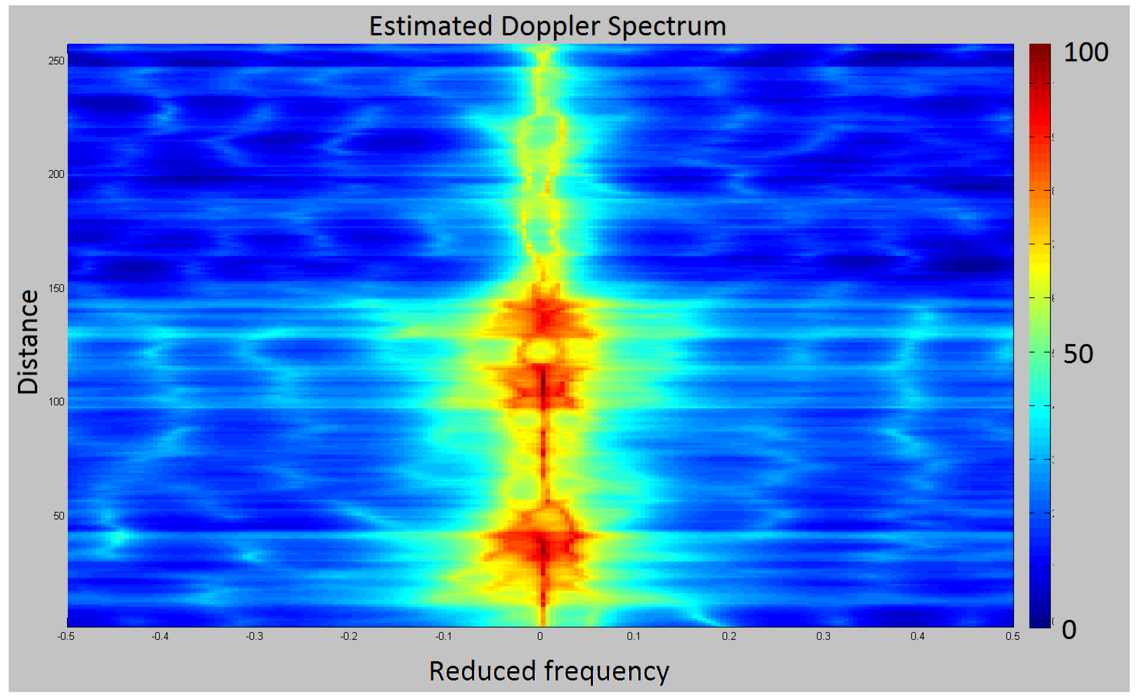
4.1. Radar Data

In space time adaptative radar processing (STAP), the signal is formed by a succession of matrices X representing the realization of a temporal and spatial process. Let B n , m + be the set of positive definite block Teoplitz matrices composed of n × n blocks of m × m matrices (PD BT). For a stationary signal, the autocorrelation matrix R is PD BT (see [5,6,14]). Authors of [5,6,14] proposed a generalization of Verblunsky coefficients and defined a parametrization of PD BT matrices,
B n , m + S y m + × D n m 1 R ( P 0 , Ω 1 , . . . , Ω m 1 ) ,
in which the metric induced by the Kähler potential is the product metric of an affine invariant metric on S y m + and m 1 times the metric of the Siegel disk, up to a scaling factor. When the signal is not Gaussian, reflection/Verblunsky coefficients in Poincaré or Siegel Disks should be normalized as described in [28] by a normalized Burg algorithm. Among other references, positive definite block Teoplitz matrices have been studied in the context of STAP-radar processing in [4,5,6].

4.2. Marginal Densities of Reflection Coefficients

In this section, we show density estimation results of the marginal parameters Ω k . For the sake of visualization, only the Siegel disk D 1 is considered. Recall that D 1 coincides with the Poincaré disk. The results are partly extracted from the conference paper [17]. Data used in the experimental tests are radar observations from THALES X-band Radar, recorded during 2014 field trials campaign at Toulouse Blagnac Airport for European FP7 UFO study (Ultra-Fast wind sensOrs for wake-vortex hazards mitigation) (see [29,30]). Data are representative of Turbulent atmosphere monitored by radar. Figure 2 illustrates the density estimation of six coefficients on the Poincaré unit disk under a rainy environment. The densities are individually re-scaled for visualization purposes. For each environment, the dataset is composed of 120 draws. The densities of the coefficients Ω k are representative of the background. This information on the background is expected to ease the detection of interesting targets.

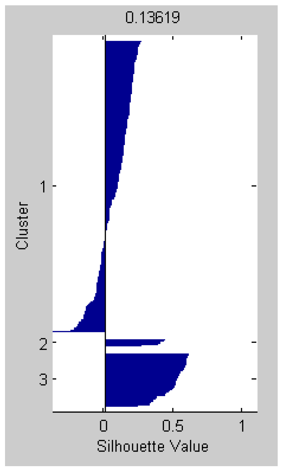
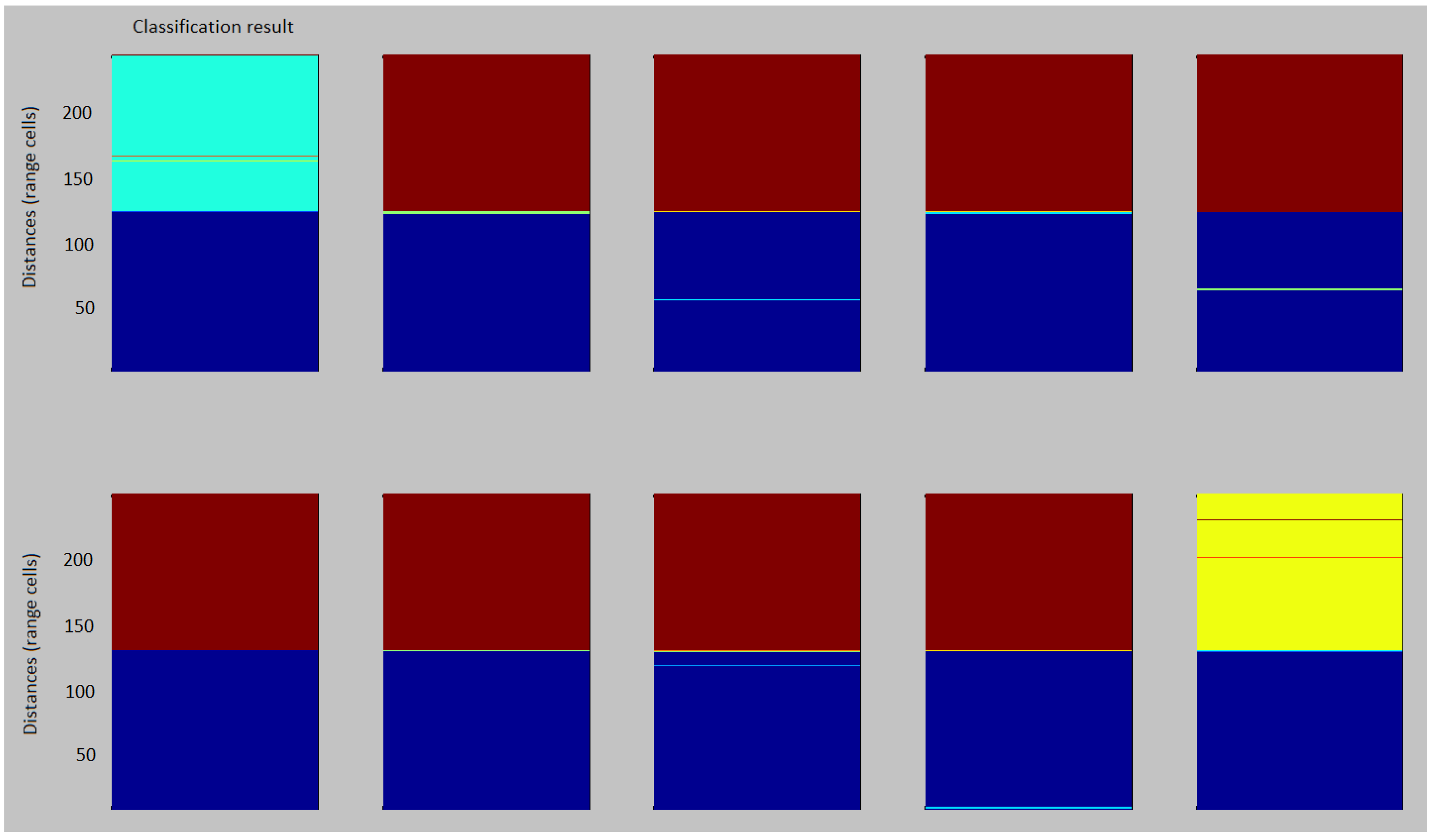
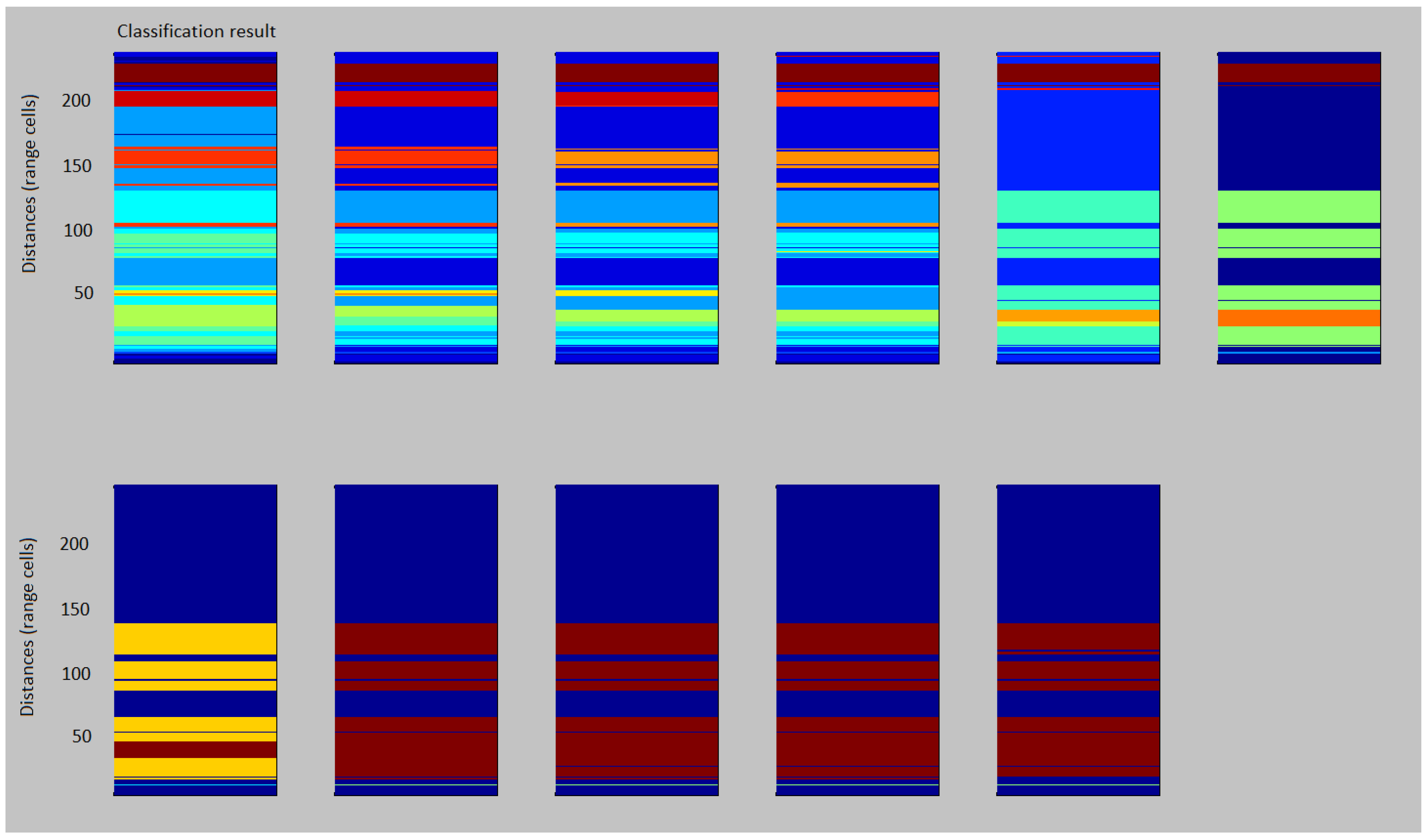
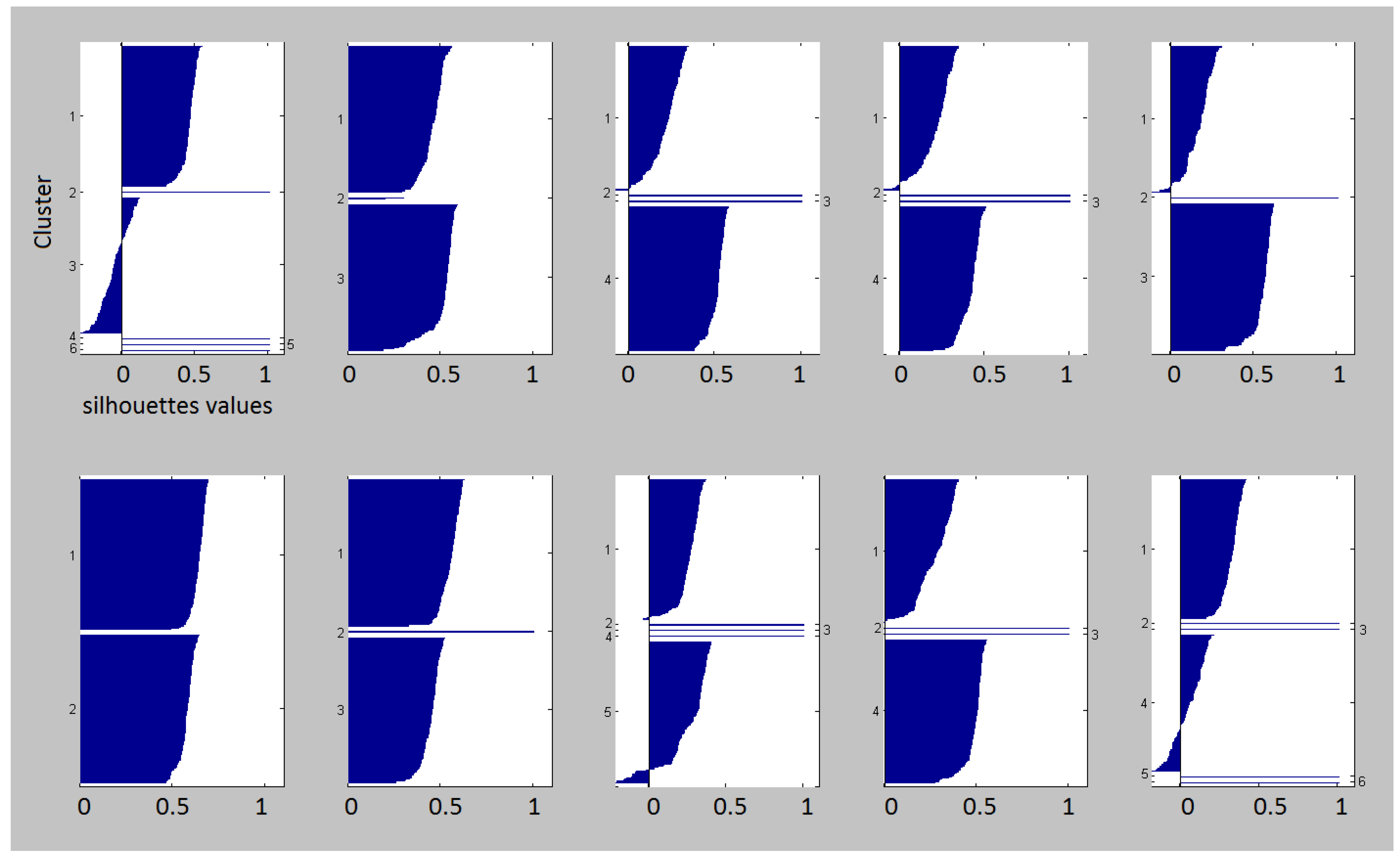
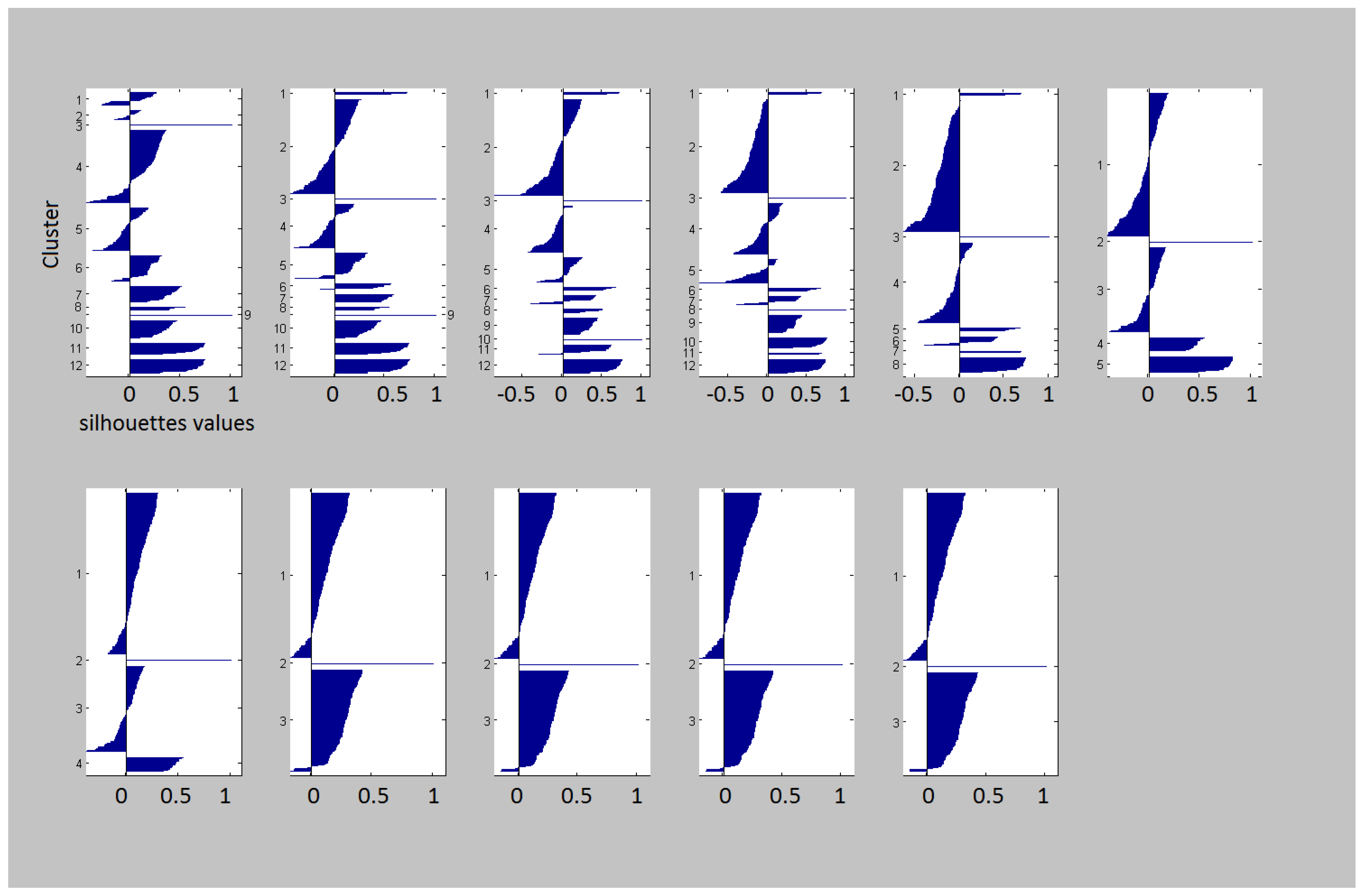
4.3. Radar Clutter Segmentation

Clutter refers to background Doppler signal related to meteorological conditions (e.g., wind in wooded areas, currents and breaking waves on water), which hinders detection of small and slow targets. At each range, a set of reflection coefficients are computed from the Doppler spectrum (see [31]). This set of coefficients is a point in the Poincaré poly-disk. From this set of points in the poly-disk, it is possible to estimate the underlying density. Segmenting clutter, i.e., determining zones of homogeneous Doppler characteristics (see Figure 3), enables the improvement of detection algorithms on each zone. The mean-shift algorithm enables segmentation of the space according to the kernel density estimation of a set of points. It was introduced by Fukunaga and Hostetler in 1975 (see [32]). It corresponds to a gradient ascent of the density estimator (see [33]) for a study of the statistical consistency of the gradient lines estimation. Each data point moves to a local mode of the density estimator, which yields as many clusters as modes. This algorithm has been generalized on manifolds in [34], and applied to radar images in [35]. It can thus be used to segment the set of points in the Poincaré poly-disk. Unfortunately, the mean-shift algorithm requires working with a kernel depending only on the distance to its barycenter, which is not the case of the kernel defined in Equation (19). Thus, the computations are performed without the use of the corrective term θ p . It is possible to solve this problem by replacing the corrective term by its average at a given radius, which leads to a kernel depending only on the distance to its barycenter. Our future work will focus on the computation of these averages. Let
f ^ r K ( x ) = c d k i = 1 k 1 r n K d ( x i , x ) 2 r 2 ,
where c n is a normalization constant. Let g = k .
The mean-shift is defined by
m ( x ) = i = 1 k 1 r n + 2 g d ( x , x i ) 2 r 2 i = 1 k 1 r n + 2 g d ( x , x i ) 2 r 2 l o g x ( x i ) f r K f r g ,
where m ( x ) is in the tangent space at x. The algorithm moves from x to e x p x ( m ( x ) ) until convergence to a local maximum. The points of the space are segmented according to the local maxima to which they converge.
In order to assess the quality of unsupervised classification, we use the notion of Silhouette, see [36], which computes for each point a proximity criterion with respect to other points of the same cluster and other points of different clusters (see Figure 4). Let x be in the cluster A. We respectively define a ( x ) = m i n y A d ( x , y ) and b ( x ) = m i n y A d ( x , y ) , the minimum distance to points of the same (resp. other) class(es). The Silhouette of x is
a ( x ) b ( x ) m a x { a ( x ) , b ( x ) } ,
which takes values between 1 and 1, respectively, when the data point is considered “badly” and “well” clustered. The average of all the silhouettes provides an indication of the relevance of the classification. One can represent graphically the silhouette profile by plotting for each class horizontal segments of the length of the silhouette value (see Figure 5).
In order to test the Riemannian Mean Shift performance, we generate simple synthetic radar clutter data. Given 250 range cells, we generate 125 cells of ground clutter (wind) centered at 0 m·s−1, of spectral width 5 m·s−1, to which we add 125 cells of rain clutter, centered at 5 m·s−1, of spectral width 10 m·s−1. This clutter is sampled 10 times and the segmentation is performed on each simulation (see Figure 6, Figure 7 and Figure 8).
It can be seen that, apart from a few outliers, the two clutters are well classified and that the algorithm was able to distinguish between two zones of different Doppler characteristics.
We then test our algorithm on real sea clutter data (see Figure 9, Figure 10 and Figure 11).
The results are more difficult to interpret in that case. The Doppler spectra are varying quite a lot along the range axis. Even though it looks over-segmented, the first classification (kernel size defined by the distance to the 10th closest neighbor point) displays the highest average silhouette value.

5. Conclusions

Three non parametric density estimation techniques have been considered. The main advantage of histograms in the Euclidean context is their simplicity of use. This makes histograms an interesting tool despite the fact that they do not present optimal convergence rates. On the Siegel space, histograms lose their simplicity advantage. They were thus not deeply studied. The orthogonal series density estimation also presents technical disadvantages on the Siegel space. Indeed, the series become integrals, which make the numerical computation of the estimator more difficult than in the Euclidean case. On the other hand, the use of the kernel density estimator does not present major differences with the Euclidean case. The convergence rate obtained in [1] can be extended to compactly supported random variables on non compact Riemannian manifolds. Furthermore, the corrective term whose computation is required to use Euclidean kernels on Riemannian manifolds turns out to have a reasonably simple expression. Our future efforts will concentrate on the use of kernel density estimation on the Siegel space in radar signal processing. As the experimental section suggests, we strongly believe that the estimation of the densities of the Ω k will provide an interesting description of the different backgrounds. This non-parametric method of density estimation should be compared with parametric ones, as “Maximum Entropy Density” (Gibbs density) on homogenesous manifold as proposed in [37] based on the works of Jean-Marie Souriau. As proposed in [38], a median-shift approach might also be investigated.

Acknowledgments

The authors would like to thank Salem Said, Michal Zidor and Dmitry Gourevitch for the help they provided in the understanding of symmetric spaces and the Siegel space.

Author Contributions

Emmanuel Chevallier carried out the mathematical development. Thibault Forget has set up the Radar clutter segmentation. Frédéric Barbaresco has introduced Poincaré/Siegel Half space and Poincaré/Siegel Disk parameterization for Radar Doppler and Space-Time Adaptive Processing based on Metric spaces deduced from Information Geometry. This parameterization has been re-used in this paper. Jesus Angulo was the Ph.D. supervisor of Emmanuel Chevallier and participates in the supervision of master thesis of Thibault Forget, both thesis are at the origin of this study. All authors have read and approved the final manuscript.

Conflicts of Interest

The authors declare no conflict of interest.

Appendix A. Demonstration of Theorem 1

Lemma A1.
Let ( M , g ) be a Riemannian manifold, let C be a compact subset of M and let U be a relatively compact open subset of M containing C. Then, there is a compact Riemannian manifold ( M , g ) such that U is an open subset of M , the inclusion i : U M is a diffeomorphism onto its image and g = g on U ¯ .
Proof. 
We can assume that M is not compact. Let f : M R be a smooth function on M which tends to + at infinity. Since U ¯ is compact, f 1 ( ] , a [ ) contains U ¯ for a large enough. By Sard Theorem, there exists a value a R such that f 1 ( a ) contains no critical point of f and such that f 1 ( ] , a [ ) contains U ¯ . It follows that N = f 1 ( ] , a ] ) is a submanifold with boundary of M. Since f tends to + at infinity, N is compact as well as its boundary N = f 1 ( { a } ) .
Call M the double of N. It is a compact manifold which contains N such that the inclusion i : N M is a diffeomorphism onto its image (see [39], Theorem 5.9 and Definition 5.10 ). Choose any metric g 0 on M . Consider two open subsets W 1 and W 2 in M and two smooth functions f 1 , f 2 : M [ 0 , 1 ] such that
U ¯ W 1 W ¯ 1 W 2 W ¯ 2 int N ,
the interior of N,
f 1 ( x ) = 1
on W ¯ 1 , vanishes outside of W 2 , and
f 2 ( x ) = 1
outside W 1 , and vanishes in U ¯ . Define g on M by
g = f 1 g + f 2 g 0
on N and
g = f 2 g 0
outside of N. Since f 1 + f 2 > 0 , g is positive definite everywhere on M . Since f 1 vanishes outside of W 2 , g is smooth on M . Finally, since f 1 = 1 and f 2 = 0 on U ¯ , g = g on U ¯ . ☐
We can now prove Theorem 1. Let X be a random variable as in Theorem 1. Following the notations of the theorem and the lemma, let U = x M , d ( x , C ) < r i n j . U is open, relatively compact and contains C. Let ( M , g ) be as in the lemma. Let f ^ and f ^ be the kernel density estimators defined on M and M , respectively. Theorem 3.1 of [1] provides the desired results for f ^ . For r r i n j , the support and the values on the support of f ^ and f ^ coincide. Thus, the desired result also holds for f ^ .

References

  1. Pelletier, B. Kernel density estimation on Riemannian manifolds. Stat. Probab. Lett. 2005, 73, 297–304. [Google Scholar] [CrossRef]
  2. Hendriks, H. Nonparametric estimation of a probability density on a Riemannian manifold using Fourier expansions. Ann. Stat. 1990, 18, 832–849. [Google Scholar] [CrossRef]
  3. Asta, D.M. Kernel Density Estimation on Symmetric Spaces. In Geometric Science of Information; Springer: Berlin/Heidelberg, Germany, 2015; Volume 9389, pp. 779–787. [Google Scholar]
  4. Barbaresco, F. Robust statistical radar processing in Fréchet metric space: OS-HDR-CFAR and OS-STAP processing in siegel homogeneous bounded domains. In Proceedings of the 2011 12th International Radar Symposium (IRS), Leipzig, Germany, 7–9 Septerber 2011.
  5. Barbaresco, F. Information Geometry of Covariance Matrix: Cartan-Siegel Homogeneous Bounded Domains, Mostow/Berger Fibration and Fréchet Median. In Matrix Information Geometry; Bhatia, R., Nielsen, F., Eds.; Springer: Berlin/Heidelberg, Germany, 2012; pp. 199–256. [Google Scholar]
  6. Barbaresco, F. Information geometry manifold of Toeplitz Hermitian positive definite covariance matrices: Mostow/Berger fibration and Berezin quantization of Cartan-Siegel domains. Int. J. Emerg. Trends Signal Process. 2013, 1, 1–87. [Google Scholar]
  7. Berezin, F.A. Quantization in complex symmetric spaces. Izv. Math. 1975, 9, 341–379. [Google Scholar] [CrossRef]
  8. Lenz, R. Siegel Descriptors for Image Processing. IEEE Signal Process. Lett. 2016, 25, 625–628. [Google Scholar]
  9. Barbaresco, F. Robust Median-Based STAP in Inhomogeneous Secondary Data: Frechet Information Geometry of Covariance Matrices. In Proceedings of the 2nd French-Singaporian SONDRA Workshop on EM Modeling, New Concepts and Signal Processing For Radar Detection and Remote Sensing, Cargese, France, 25–28 May 2010.
  10. Degurse, J.F.; Savy, L.; Molinie, J.P.; Marcos, S. A Riemannian Approach for Training Data Selection in Space-Time Adaptive Processing Applications. In Proceedings of the 2013 14th International Radar Symposium (IRS), Dresden, Germany, 19–21 June 2013; Volume 1, pp. 319–324.
  11. Degurse, J.F.; Savy, L.; Marcos, S. Information Geometry for radar detection in heterogeneous environments. In Proceedings of the 33rd International Workshop on Bayesian Inference and Maximum Entropy Methods in Science and Engineering, Amboise, France, 21–26 September 2014.
  12. Barbaresco, F. Koszul Information Geometry and Souriau Geometric Temperature/Capacity of Lie Group Thermodynamics. Entropy 2014, 16, 4521–4565. [Google Scholar] [CrossRef]
  13. Barbaresco, F. New Generation of Statistical Radar Processing based on Geometric Science of Information: Information Geometry, Metric Spaces and Lie Groups Models of Radar Signal Manifolds. In Proceedings of the 4th French-Singaporian Radar Workshop SONDRA, Lacanau, France, 23 May 2016.
  14. Jeuris, B.; Vandebril, R. The Kahler mean of Block-Toeplitz matrices with Toeplitz structured block. SIAM J. Matrix Anal. Appl. 2015, 37, 1151–1175. [Google Scholar] [CrossRef]
  15. Huckemann, S.; Kim, P.; Koo, J.; Munk, A. Mobius deconvolution on the hyperbolic plan with application to impedance density estimation. Ann. Stat. 2010, 38, 2465–2498. [Google Scholar] [CrossRef]
  16. Asta, D.; Shalizi, C. Geometric network comparison. 2014; arXiv:1411.1350. [Google Scholar]
  17. Chevallier, E.; Barbaresco, F.; Angulo, J. Probability density estimation on the hyperbolic space applied to radar processing. In Geometric Science of Information; Springer: Berlin/Heidelberg, Germany, 2015; pp. 753–761. [Google Scholar]
  18. Said, S.; Bombrun, L.; Berthoumieu, Y. New Riemannian Priors on the Univariate Normal Model. Entropy 2014, 16, 4015–4031. [Google Scholar] [CrossRef]
  19. Said, S.; Hatem, H.; Bombrun, L.; Baba, C.; Vemuri, B.C. Gaussian distributions on Riemannian symmetric spaces: Statistical learning with structured covariance matrices. 2016; arXiv:1607.06929. [Google Scholar]
  20. Terras, A. Harmonic Analysis on Symmetric Spaces and Applications II; Springer: Berlin/Heidelberg, Germany, 2012. [Google Scholar]
  21. Siegel, C.L. Symplectic geometry. Am. J. Math. 1943, 65. [Google Scholar] [CrossRef]
  22. Helgason, S. Differential Geometry, Lie Groups, and Symmetric Spaces; Academic Press: Cambridge, MA, USA, 1979. [Google Scholar]
  23. Cannon, J.W.; Floyd, W.J.; Kenyon, R.; Parry, W.R. Hyperbolic geometry. In Flavors of Geometry; Cambridge University Press: Cambridge, UK, 1997; Volume 31, pp. 59–115. [Google Scholar]
  24. Bhatia, R. Matrix Analysis. In Graduate Texts in Mathematics-169; Springer: Berlin/Heidelberg, Germany, 1997. [Google Scholar]
  25. Kim, P.; Richards, D. Deconvolution density estimation on the space of positive definite symmetric matrices. In Nonparametric Statistics and Mixture Models: A Festschrift in Honor of Thomas P. Hettmansperger; World Scientific Publishing: Singapore, 2008; pp. 147–168. [Google Scholar]
  26. Loubes, J.-M.; Pelletier, B. A kernel-based classifier on a Riemannian manifold. Stat. Decis. 2016, 26, 35–51. [Google Scholar] [CrossRef]
  27. Gangolli, R.; Varadarajan, V.S. Harmonic Analysis of Spherical Functions on Real Reductive Groups; Springer: Berlin/Heidelberg, Germany, 1988. [Google Scholar]
  28. Decurninge, A.; Barbaresco, F. Robust Burg Estimation of Radar Scatter Matrix for Mixtures of Gaussian Stationary Autoregressive Vectors. 2016; arxiv:1601.02804. [Google Scholar]
  29. Barbaresco, F. Eddy Dissipation Rate (EDR) retrieval with ultra-fast high range resolution electronic-scanning X-band airport radar: Results of European FP7 UFO Toulouse Airport trials. In Proceedings of the 2015 16th International Radar Symposium, Dresden, Germany, 24–26 June 2015.
  30. Oude Nijhuis, A.C.P.; Thobois, L.P.; Barbaresco, F. Monitoring of Wind Hazards and Turbulence at Airports with Lidar and Radar Sensors and Mode-S Downlinks: The UFO Project; Bulletin of the American Meteorological Society, 2016; submitted for publication. [Google Scholar]
  31. Barbaresco, F.; Forget, T.; Chevallier, E.; Angulo, J. Doppler spectrum segmentation of radar sea clutter by mean-shift and information geometry metric. In Proceedings of the 17th International Radar Symposium (IRS), Krakow, Poland, 10–12 May 2016; pp. 1–6.
  32. Fukunaga, K.; Hostetler, L.D. The Estimation of the Gradient of a Density Function, with Applications in Pattern Recognition. Proc. IEEE Trans. Inf. Theory 1975, 21, 32–40. [Google Scholar] [CrossRef]
  33. Arias-Castro, E.; Mason, D.; Pelletier, B. On the estimation of the gradient lines of a density and the consistency of the mean-shift algorithm. J. Mach. Learn. Res. 2000, 17, 1–28. [Google Scholar]
  34. Subbarao, R.; Meer, P. Nonlinear Mean Shift over Riemannian Manifolds. Int. J. Comput. Vis. 2009, 84. [Google Scholar] [CrossRef]
  35. Wang, Y.H.; Han, C.Z. PolSAR Image Segmentation by Mean Shift Clustering in the Tensor Space. Acta Autom. Sin. 2010, 36, 798–806. [Google Scholar] [CrossRef]
  36. Rousseeuw, P. Silhouettes: A graphical aid to the interpretation and validation of cluster analysis. J. Comput. Appl. Math. 1987, 1, 53–65. [Google Scholar] [CrossRef]
  37. Barbaresco, F. Geometric Theory of Heat from Souriau Lie Groups Thermodynamics and Koszul Hessian Geometry: Applications in Information Geometry for Exponential Families. Entropy 2016, 18, 386. [Google Scholar] [CrossRef]
  38. Wanga, Y.; Huang, X.; Wua, L. Clustering via geometric median shift over Riemannian manifolds. Inf. Sci. 2013, 220, 292–305. [Google Scholar] [CrossRef]
  39. Munkres, J.R. Elementary Differential Topology. In Annals of Mathematics Studies-54; Princeton University Press: Princeton, NJ, USA, 1967. [Google Scholar]
Figure 1. M is a Riemannian manifold, and T x M is its tangent space at x. The exponential application induces a volume change θ x between T x M and M .
Entropy 18 00396 g001
Figure 2. Estimation of the density of six coefficients Ω k under rainy conditions. The expression of the used kernel is K ( x ) = 3 π ( 1 x 2 ) 2 1 x < 1 . Densities are rescaled for visual purposes.
Entropy 18 00396 g002
Figure 3. Mean and width variability of sea clutter Doppler spectrum.
Entropy 18 00396 g003
Figure 4. Intra and inter cluster distances.
Entropy 18 00396 g004
Figure 5. Example of silhouette.
Entropy 18 00396 g005
Figure 6. Autoregressive spectra.
Entropy 18 00396 g006
Figure 7. Classification results (one color per cluster).
Entropy 18 00396 g007
Figure 8. Silhouettes.
Entropy 18 00396 g008
Figure 9. Autoregressive spectrum.
Entropy 18 00396 g009
Figure 10. Classification results for varying radii size in the density estimator (10 to 20 closest neighbours).
Entropy 18 00396 g010
Figure 11. Silhouettes.
Entropy 18 00396 g011

