Article

Generalized Combination Complex Synchronization for Fractional-Order Chaotic Complex Systems

College of Control Science and Engineering, Shandong University, Jinan 250061, China
*
Author to whom correspondence should be addressed.
Entropy 2015, 17(8), 5199-5217; https://doi.org/10.3390/e17085199
Submission received: 10 March 2015 / Revised: 29 June 2015 / Accepted: 17 July 2015 / Published: 24 July 2015
(This article belongs to the Special Issue Recent Advances in Chaos Theory and Complex Networks)

Abstract

:
Based on two fractional-order chaotic complex drive systems and one fractional-order chaotic complex response system with different dimensions, we propose generalized combination complex synchronization. In this new synchronization scheme, there are two complex scaling matrices that are non-square matrices. On the basis of the stability theory of fractional-order linear systems, we design a general controller via active control. Additionally, by virtue of two complex scaling matrices, generalized combination complex synchronization between fractional-order chaotic complex systems and real systems is investigated. Finally, three typical examples are given to demonstrate the effectiveness and feasibility of the schemes.

1. Introduction

Fractional-order systems have attracted noticeable interest and have been well studied for their potential applications in assorted fields, like engineering, physics, finance, chemistry and bioengineering [1,2,3,4,5]. Recently, the research on fractional-order chaotic systems has become a hot issue. The efforts have been devoted to chaotic behavior, chaos control and chaos synchronization. Some fractional-order systems behave chaotically or hyperchaotically, such as the fractional-order Chua system [6], the fractional-order hyperchaotic Chen system [7], the fractional-order hyperchaotic Rössler system [8], and so on. Most recently, many authors have found some fractional-order chaotic systems, including the fractional-order reverse butterfly-shaped chaotic system [9], the fractional-order stretch-twist-fold (STF) flow chaotic system [10], a four-dimensional fractional-order chaotic system without an equilibrium point [11], etc. Synchronization of fractional-order chaotic systems has been widely investigated due to its potential applications in secure communication, encryption, signal and control processing [9,10,12,13,14]. Therefore, a variety of effective methods have been proposed to synchronize various fractional-order chaotic systems. For instance, Agrawal et al. [15] realized synchronization of fractional-order chaotic systems via active control. A linear control method was proposed to synchronize the fractional-order chaotic systems in [16]. By employing the active control method, the phase and anti-phase synchronization of two fractional-order chaotic systems were studied in [17]. Si et al. [18] achieved the projective synchronization between two fractional-order chaotic systems with non-identical orders. Some more attempts to realize the synchronization of fractional-order chaotic systems can be found in [19,20].
Recently, with the development of fractional-order real systems and integer-order complex systems, fractional-order chaotic complex systems have attracted a great deal of attention, and many interesting and important results have been researched. For example, the fractional-order complex Lorenz system and its complete synchronization were discussed in [21]. Luo and Wang presented the fractional-order complex Chen system and applied its hybrid synchronization to digital secure communication [22]. The fractional-order complex T system was presented, and its function projective synchronization was realized in [23]. Jiang et al. [24] introduced the fractional-order complex Lü system and achieved its anti-synchronization. Complex modified hybrid projective synchronization was investigated between the fractional-order complex chaos and real hyper-chaos in [25].
However, in the aforementioned literature on the synchronization of the fractional-order chaotic systems, many authors are concerned with the usual drive-response synchronization within one drive system and one response system, and three or more chaotic systems are rarely involved. As a matter of fact, synchronization of multi-chaotic systems can enhance the security in communication, because the transmitted signals can be split into several parts loaded in the different drive systems or the same drive system with different initial conditions. Therefore, many researchers have made an endeavor to analyze the synchronization of multi-chaotic systems and present some new types of synchronization, including combination synchronization [26,27,28], combination complex synchronization [29], combination-combination synchronization [30,31], compound synchronization [32], and so forth. Amongst the above-mentioned synchronization, combination complex synchronization, characterized by two scaling matrices that three chaotic systems synchronize proportionally, was proposed and studied on the basis of three integer-order chaotic complex systems with the same dimensions.
To the best of our knowledge, there are few results on combination complex synchronization of the fractional-order chaotic complex systems with different dimensions. Motivated by this, we proposed generalized combination complex synchronization among three different dimensional fractional-order chaotic complex systems. By virtue of the stability of the fractional-order linear systems, some sufficient conditions for generalized combination complex synchronization are obtained. Besides, we investigate generalized combination complex synchronization between the fractional-order real chaos and complex chaos. There are some kinds of synchronization that are special cases from our definition, which are complex projective synchronization, combination synchronization and combination complex synchronization. Consequently, our work will extend previous results.
The remainder of this paper is organized as follows. Section 2 recalls the relevant definitions and stability results of the fractional-order systems. In Section 3, we present generalized combination complex synchronization and design a scheme to realize the new form of chaos synchronization. By means of two scaling matrices, we establish a link between fractional-order chaotic real systems and chaotic complex systems with different dimensions. Section 4 provides three examples to exhibit the feasibility and effectiveness of the proposed control technique. Finally, some conclusions are drawn in Section 5.

2. Preliminaries

In this section, we introduce mathematical definitions of the fractional derivative and the stability results of the fractional-order systems. The fractional-order integro-differential operator is the generalized concept of the integer-order integro-differential operator, which can be denoted by a general fundamental operator as follows:
a D t α = d α d t α , R ( α ) > 0 , 1 , R ( α ) = 0 , a t ( d τ ) α , R ( α ) < 0 ,
where α is the fractional-order, which can be a complex number, R ( α ) is the real part of α and a and t are the limits of the operation. As we know, there are several definitions of fractional derivatives, including the Grunwald–Letnikov definition, the Riemann–Liouville definition and the Caputo definition.
The Grunwald–Letnikov (GL) derivative with fractional order α is given by:
a G D t α f ( t ) = lim h 0 f h ( α ) ( t ) = lim h 0 h α i = 0 t α h ( 1 ) i α i f ( t i h ) ,
where [ · ] means the integer part.
The Riemann–Liouville (RL) fractional derivative is defined by:
a R D t α f ( t ) = 1 Γ ( n α ) d n d t n a t f ( τ ) ( t τ ) α n + 1 d τ , n 1 < α < n ,
where Γ ( · ) is the Gamma function Γ ( τ ) = 0 t τ 1 e t d t .
The Caputo (C) fractional derivative [33] is defined as:
a C D t α f ( t ) = 1 Γ ( n α ) t 0 t f ( n ) ( τ ) ( t τ ) α n + 1 d τ , n 1 < α < n .
In the rest of this paper, the notation D * α is chosen as the Riemann–Liouville derivative operator a R D t α , and we mainly consider the order 0 < α < 1 .
Consider a fractional-order autonomous system:
D * α x ( t ) = A x ( t ) , x ( 0 ) = x 0 ,
where 0 < α < 1 , x R n and A R n × n .
The stability results for the fractional-order linear system [34] are given as follows:
Lemma 1.
System (1) is:
(I)
Asymptotically stable if and only if:
| arg ( λ i ( A ) ) | > α π / 2 , ( i = 1 , 2 , , n ) ,
where arg ( λ i ( A ) ) denotes the argument of the eigenvalue λ i of A. In this case, the component of the state decay towards to zero like t α .
(II)
Stable if and only if:
| arg ( λ i ( A ) ) | α π / 2 , ( i = 1 , 2 , , n ) ,
and those critical eigenvalues λ i that satisfy | arg ( λ i ( A ) ) | = α π / 2 have geometric multiplicity one.

3. The Scheme of Generalized Combination Complex Synchronization

In this section, we propose generalized combination complex synchronization and design a general controller.

3.1. The Definition of Generalized Combination Complex Synchronization

The first drive system is an n 1 -dimensional fractional-order chaotic complex system, which isdescribed as:
D * α x ( t ) = D * α x r + j D * α x i = A x + f ( x ) ,
and the second drive system is an n 2 -dimensional chaotic complex system, which is given as:
D * α y ( t ) = D * α y r + j D * α y i = B y + g ( y ) ,
while the response system is an n-dimensional complex system, which is assumed as:
D * α z ( t ) = D * α z r + j D * α z i = C z + h ( z ) + U ( x , y , z ) ,
where x = x r + j x i C n 1 × 1 , y = y r + j y i C n 2 × 1 and z = z r + j z i C n × 1 are the state complex vectors, A R n 1 × n 1 , B R n 2 × n 2 and C R n × n are parameter matrices, while f, g and h are nonlinear complex functions and U is a designed controller in the following.
Remark 1.
Many fractional-order chaotic complex systems can be depicted by (2), such as the fractional-order complex Lorenz system, the fractional-order complex Chen system, the fractional-order complex T system, the fractional-order complex Lü system, and so forth.
Based on two complex drive systems and one complex response system with different dimensions, we introduce the definition of generalized combination complex synchronization.
Definition 1.
For two drive systems, (2) and (3), and one response system, (4), it is said to be generalized combination complex synchronization if there exist two complex matrices D 1 = D 1 r + j D 1 i C n × n 1 and D 2 = D 2 r + j D 2 i C n × n 2 , such that:
lim t | | e ( t ) | | = lim t | | z ( t ) D 1 x ( t ) D 2 y ( t ) | | = 0 ,
where | | . | | is the matrix norm, e ( t ) = e r ( t ) + j e i ( t ) is called the error vector and e r = z r D 1 r x r + D 1 i x i D 2 r y r + D 2 i y i , e i = z i D 1 r x i D 1 i x r D 2 r y i D 2 i y r , the complex matrices D 1 and D 2 are called the scaling matrices.
Remark 2.
If the dimensions of two drive systems, (2) and (3), are equal to that of the response system, (4), i.e., n = n 1 = n 2 , then combination complex synchronization will appear.
Remark 3.
If the scaling matrix D 1 = O n × n 1 or D 2 = O n × n 2 , then we can achieve complex projective synchronization. If D 1 i = O n × n 1 or D 2 i = O n × n 2 , then combination synchronization can be carried out. If D 1 = O n × n 1 and D 2 = O n × n 2 , then the synchronization problem will be changed into the chaoscontrol problem.
The purpose of this paper is to design suitable controllers, such that the fractional-order chaotic nonlinear systems can achieve generalized combination complex synchronization.

3.2. A General Method for Generalized Combination Complex Synchronization

Theorem 1.
Assume that the control law is chosen as follows:
U r = C ( D 1 r x r D 1 i x i + D 2 r y r D 2 i y i ) h r ( z ) + D 1 r ( A x r + f r ( x ) ) D 1 i ( A x i + f i ( x ) ) + D 2 r ( B y r + g r ( y ) ) D 2 i ( B y i + g i ( y ) ) K e r , U i = C ( D 1 r x i + D 1 i x r + D 2 r y i + D 2 i y r ) h i ( z ) + D 1 r ( A x i + f i ( x ) ) + D 1 i ( A x r + f r ( x ) ) + D 2 r ( B y i + g i ( y ) ) + D 2 i ( B y r + g r ( y ) ) K e i .
where K R n × n is a control gain matrix. Then, we achieve generalized combination complex synchronization between two drive systems, (2) and (3), and one response system, (4), if and only if all eigenvalues λ i of C K lie in the region | arg ( λ i ( C K ) ) | > α π / 2 ( i = 1 , 2 , , n ).
Proof.
From Definition 1, we obtain the error vector between Systems (2)–(4) as follows:
e ( t ) = e r ( t ) + j e i ( t )   = z r D 1 r x r + D 1 i x i D 2 r y r + D 2 i y i + j [ z i D 1 r x i D 1 i x r D 2 r y i D 2 i y r ] .
The fractional derivative of the error system (6) can be expressed as:
D * α e ( t ) = D * α e r ( t ) + j D * α e i ( t ) = D * α z r D 1 r D * α x r + D 1 i D * α x i D 2 r D * α y r + D 2 i D * α y i + j [ D * α z i D 1 r D * α x i D 1 i D * α x r D 2 r D * α y i D 2 i D * α y r ] .
Combining Systems (2)–(4), we obtain:
D * α e r ( t ) = C z r + h r ( z ) + U r D 1 r ( A x r + f r ( x ) ) + D 1 i ( A x i + f i ( x ) ) D 2 r ( B y r + g r ( y ) ) + D 2 i ( B y i + g i ( y ) ) , D * α e i ( t ) = C z i + h i ( z ) + U i D 1 r ( A x i + f i ( x ) ) D 1 i ( A x r + f r ( x ) ) D 2 r ( B y i + g i ( y ) ) D 2 i ( B y r + g r ( y ) ) .
Substituting (5) into (11), the error complex dynamical system is written as:
D * α e r ( t ) = ( C K ) e r , D * α e i ( t ) = ( C K ) e i .
Since | arg ( λ i ( C K ) ) | > α π / 2 , according to Lemma 1, the error vector e ( t ) asymptotically converges to zero as t . Therefore, generalized combination complex synchronization betweenSystems (2)–(4) is achieved. The proof is complete.
In what follows, we discuss generalized combination complex synchronization between three different dimensional fractional-order real chaos and complex chaos. Now, we consider the following three cases.
Corollary 1.
Suppose that two drive systems, (2) and (3), are chaotic real systems, i.e., x R n 1 × 1 , y R n 2 × 1 , and one response system is a chaotic complex system, (4), i.e., z C n × 1 . For two given scaling matrices D 1 C n × n 1 and D 2 C n × n 2 , the errors are defined as:
e r ( t ) = z r D 1 r x D 2 r y , e i ( t ) = z i D 1 i x D 2 i y .
Then, generalized combination complex synchronization between two drive real systems, (2) and (3), and one response complex system, (4), will occur with the designed controller:
U r = C ( D 1 r x + D 2 r y ) h r ( z ) + D 1 r ( A x + f ( x ) ) + D 2 r ( B y + g ( y ) ) K e r , U i = C ( D 1 i x + D 2 i y ) h i ( z ) + D 1 i ( A x + f ( x ) ) + D 2 i ( B y + g ( y ) ) K e i ,
where K R n × n and all eigenvalues λ i of C K satisfy | arg ( λ i ( C K ) ) | > α π / 2 ( i = 1 , 2 , , n ) .
Corollary 2.
Assume that System (2) is a chaotic real system and System (3) is a chaotic complex system, i.e., x R n 1 × 1 , y C n 2 × 1 , while the response system is a chaotic complex system, (4), i.e., z C n × 1 . The synchronization errors with the given scaling matrices D 1 C n × n 1 and D 2 C n × n 2 aredepicted as:
e r ( t ) = z r D 1 r x D 2 r y r + D 2 i y i , e i ( t ) = z i D 1 i x D 2 r y i D 2 i y r .
Then, two drive systems, (2) and (3), and one response system, (4), can realize generalized combination complex synchronization with the following control law:
U r = C ( D 1 r x + D 2 r y r D 2 i y i ) h r ( z ) + D 1 r ( A x + f ( x ) ) + D 2 r ( B y r + g r ( y ) ) D 2 i ( B y i + g i ( y ) ) K e r , U i = C ( D 1 r x + D 2 r y i + D 2 i y r ) h i ( z ) + D 1 r ( A x + f ( x ) ) + D 2 r ( B y i + g i ( y ) ) + D 2 i ( B y r + g r ( y ) ) K e i ,
where K R n × n and all eigenvalues λ i of C K lie in the region | arg ( λ i ( C K ) ) | > α π / 2   ( i = 1 , 2 , , n ) .
Corollary 3.
Suppose that two drive systems, (2) and (3), are chaotic complex systems, i.e., x C n 1 × 1 , y C n 2 × 1 , and the response system, (4), is a chaotic real system, where z R n × 1 . Since z ( t ) is real, we select a real controller U to ensure synchronization of real parts and avoid increasing the imaginary parts of the response system. Therefore, the error vector is introduced as:
e ( t ) = z D 1 r x r + D 1 i x i D 2 r y r + D 2 i y i .
If a real controller is designed as:
U = h ( z ) C ( D 1 r x r D 1 i x i + D 2 r y r D 2 i y i ) + D 1 r ( A x r + f r ( x ) ) D 1 i ( A x i + f i ( x ) ) + D 2 r ( B y r + g r ( y ) ) D 2 i ( B y i + g i ( y ) ) K e ,
where K R n × n and all eigenvalues λ i of C K satisfy | arg ( λ i ( C K ) ) | > α π / 2   ( i = 1 , 2 , , n ) , then two drive complex systems, (2) and (3), and one response real system, (4), are the generalized combination complex synchronization of real parts.
Additionally, from Theorem 1, we obtain control laws to achieve complex projective synchronization and chaos control.
Corollary 4.
(I) Assume D 1 = O n × n 1 . If the controller is designed as follows:
U r = C ( D 2 r y r D 2 i y i ) h r ( z ) + D 2 r ( B y r + g r ( y ) ) D 2 i ( B y i + g i ( y ) ) K e r , U i = C ( D 2 r y i + D 2 i y r ) h i ( z ) + D 2 r ( B y i + g i ( y ) ) + D 2 i ( B y r + g r ( y ) ) K e i ,
then we achieve complex projective synchronization between two different dimensional systems, (3) and (4), if and only if all eigenvalues λ i of C K satisfy | arg ( λ i ( C K ) ) | > α π / 2 , K R n × n , ( i = 1 , 2 , , n ) .
(II) Assume D 2 = O n × n 2 . If the controller is designed as follows:
U r = C ( D 1 r x r D 1 i x i ) h r ( z ) + D 1 r ( A x r + f r ( x ) ) D 1 i ( A x i + f i ( x ) ) K e r , U i = C ( D 1 r x i + D 1 i x r ) h i ( z ) + D 1 r ( A x i + f i ( x ) ) + D 1 i ( A x r + f r ( x ) ) K e i ,
then we carry out complex projective synchronization between two different dimensional systems, (2) and (4), if and only if all eigenvalues λ i of C K satisfy | arg ( λ i ( C K ) ) | > α π / 2 , K R n × n , ( i = 1 , 2 , , n ) .
Corollary 5.
Suppose two scaling matrices D 1 = O n × n 1 and D 2 = O n × n 2 . If the control law is given as:
U r = h r ( z ) K e r , U i = h i ( z ) K e i ,
where K R n × n and all eigenvalues λ i of C K lie in the region | arg ( λ i ( C K ) ) | > α π / 2   ( i = 1 , 2 , , n ) , then the equilibrium point of the response system, (4), is asymptotically stable.

4. Numerical Simulations

In this section, three examples are performed to illustrate the validity and feasibility of the proposed schemes. Firstly, we work out generalized combination complex synchronization between the fractional-order complex Lorenz system, the fractional-order complex Lü system and the fractional-order complex Chen system.

4.1. Synchronization among Three Fractional-Order Chaotic Complex Systems

Now, let us consider the fractional-order complex Lorenz system as the first drive system:
D * α x 1 ( t ) = a 1 ( x 2 x 1 ) , D * α x 2 ( t ) = a 2 x 1 x 2 x 1 x 3 , D * α x 3 ( t ) = 1 2 ( x ¯ 1 x 2 + x 1 x ¯ 2 ) a 3 x 3 ,
and the fractional-order complex Lü system as the second drive system:
D * α y 1 ( t ) = b 1 ( y 2 y 1 ) , D * α y 2 ( t ) = y 1 y 3 + b 2 y 2 , D * α y 3 ( t ) = 1 2 ( y ¯ 1 y 2 + y 1 y ¯ 2 ) b 3 y 3 ,
while the response system is the fractional-order complex Chen system:
D * α z 1 ( t ) = c 1 ( z 2 z 1 ) + U 1 , D * α z 2 ( t ) = ( c 2 c 1 ) z 1 z 1 z 3 + c 2 z 2 + U 2 , D * α z 3 ( t ) = 1 2 ( z ¯ 1 z 2 + z 1 z ¯ 2 ) c 3 z 3 + U 3 ,
where A = a 1 a 1 0 a 2 1 0 0 0 a 3 , B = b 1 b 1 0 0 b 2 0 0 0 b 3 , C = c 1 c 1 0 c 2 c 1 c 2 0 0 0 c 3 , f ( x ) = 0 x 1 x 3 1 2 ( x ¯ 1 x 2 + x 1 x ¯ 2 ) , g ( y ) = 0 y 1 y 3 1 2 ( y ¯ 1 y 2 + y 1 y ¯ 2 ) , h ( z ) = 0 z 1 z 3 1 2 ( z ¯ 1 z 2 + z 1 z ¯ 2 ) ; x 1 = x 1 r + j x 1 i , x 2 = x 2 r + j x 2 i , y 1 = y 1 r + j y 1 i , y 2 = y 2 r + j y 2 i , z 1 = z 1 r + j z 1 i and z 2 = z 2 r + j z 2 i are complex variables, x 3 , y 3 and z 3 are real variables and U 1 = u 1 + j u 2 , U 2 = u 3 + j u 4 and U 3 = u 5 are complex and real control functions, respectively. Systems (8)–(10) behave chaotically with the given parameters α = 0 . 95 , ( a 1 , a 2 , a 3 ) = ( 10 , 180 , 1 ) , ( b 1 , b 2 , b 3 ) = ( 42 , 22 , 5 ) and ( c 1 , c 2 , c 3 ) = ( 35 , 28 , 3 ) , respectively; see Figure 1, Figure 2 and Figure 3. In what follows, we will select the above system parameters and fractional orders in our synchronization analysis.
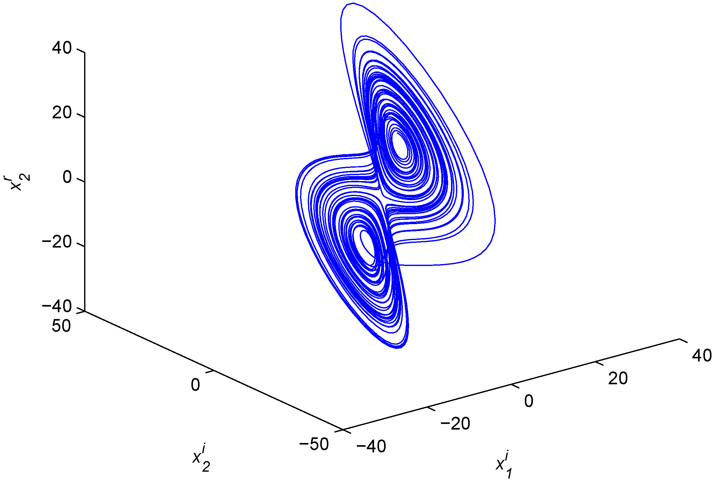
Figure 1. Chaotic attractor of the fractional-order complex Lorenz system.
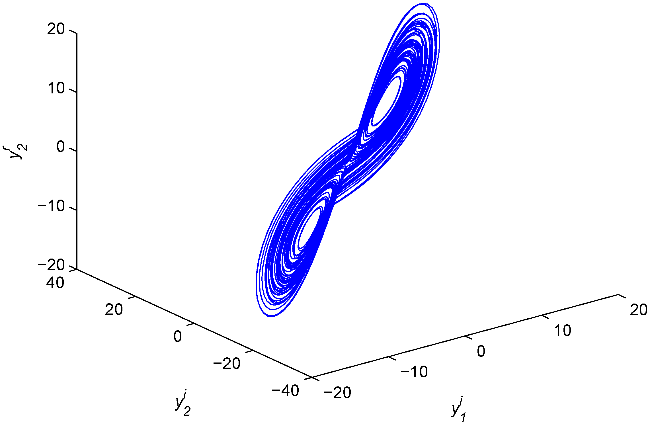
Entropy 17 05199 g001
Figure 2. Chaotic attractor of the fractional-order complex Lü system.
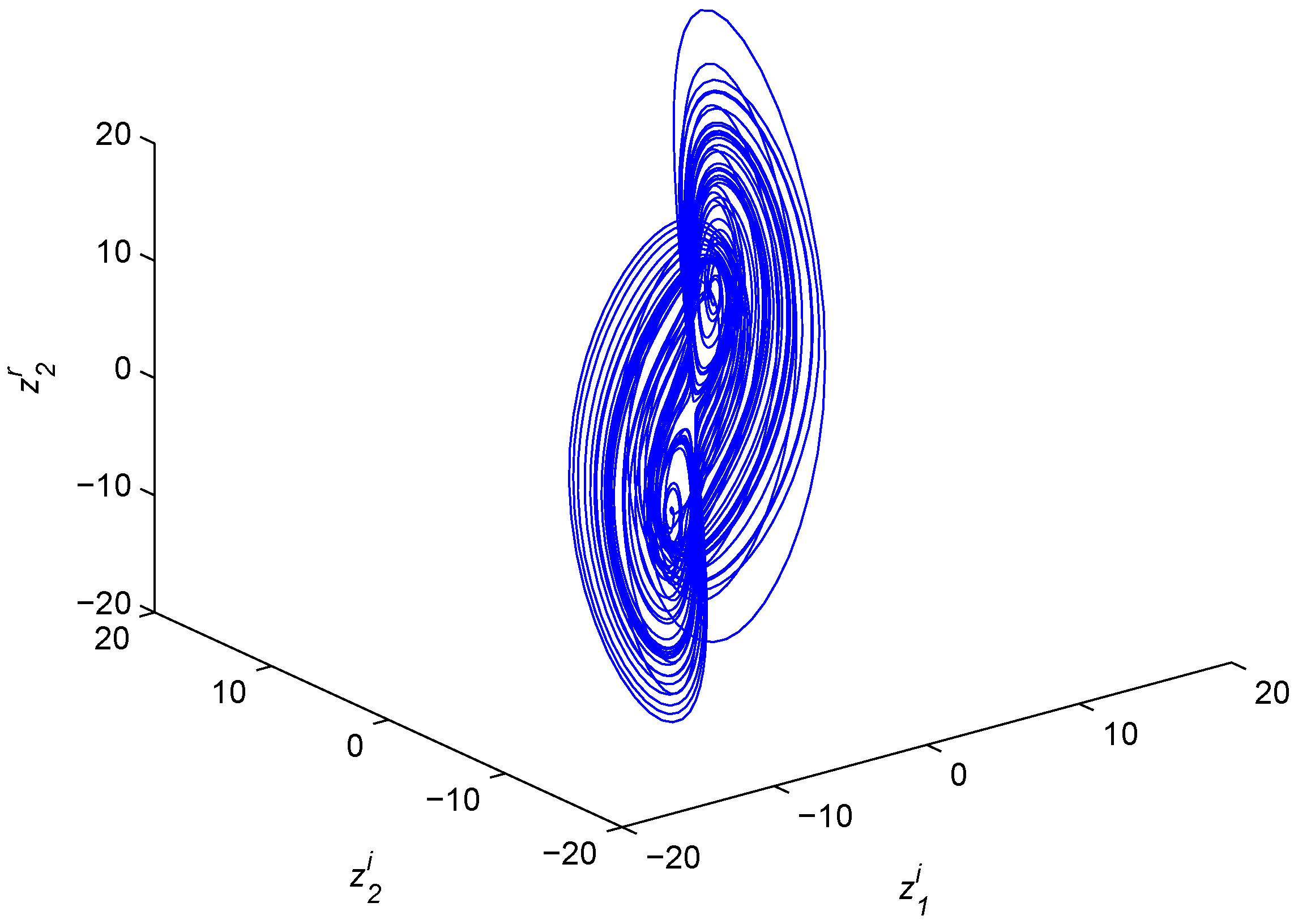
Entropy 17 05199 g002
Figure 3. Chaotic attractor of the fractional-order complex Chen system.
Entropy 17 05199 g003
Assume that D 1 = j 0 0 0 j 0 0 0 1 , D 2 = j 0 0 0 j 0 0 0 1 . Then, we obtain the synchronization error functions as follows:
e 1 ( t ) = e 1 r + j e 1 i = z 1 r + x 1 i + y 1 i + j ( z 1 i x 1 r y 1 r ) , e 2 ( t ) = e 2 r + j e 2 i = z 2 r x 2 i + y 2 i + j ( z 2 i + x 2 r y 2 r ) , e 3 ( t ) = z 3 x 3 + y 3 .
A control matrix is chosen as K = 29 31 1 5 30 0 0 0 7 ; then, we have C K = 6 4 1 2 2 0 0 0 10 for the choice of ( c 1 , c 2 , c 3 ) = ( 35 , 28 , 3 ) . It is not difficult to see that all eigenvalues of C K are λ 1 , 2 = 4 ± 2 j and λ 3 = 10 , which satisfy | arg ( λ i ( C K ) ) | > α π / 2 , ( i = 1 , 2 , 3 ) .
According to Theorem 1, the controller is designed as:
u 1 = ( a 1 c 1 ) x 1 i + ( b 1 c 1 ) ( y 1 i y 2 i ) ( a 1 + c 1 ) x 2 i + 29 e 1 r 31 e 2 r + e 3 , u 2 = ( c 1 a 1 ) x 1 r + ( c 1 b 1 ) ( y 1 r y 2 r ) + ( a 1 + c 1 ) x 2 r + 29 e 1 i 31 e 2 i , u 3 = ( c 2 c 1 + a 2 ) x 1 i + ( c 2 c 1 ) y 1 i + ( c 2 b 2 ) y 2 i ( 1 + c 2 ) x 2 i x 1 i x 3 + y 1 i y 3 + z 1 r z 3 + 5 e 1 r 30 e 2 r , u 4 = ( c 1 c 2 a 2 ) x 1 r + ( c 1 c 2 ) y 1 r + ( b 2 c 2 ) y 2 r + ( 1 + c 2 ) x 2 r + x 1 r x 3 y 1 r y 3 + z 1 i z 3 + 5 e 1 i 30 e 2 i , u 5 = ( c 3 a 3 + 7 ) x 3 + ( b 3 c 3 7 ) y 3 7 z 3 z 1 r z 2 r z 1 i z 2 i + x 1 r x 2 r + x 1 i x 2 i y 1 r y 2 r y 1 i y 2 i .
In the numerical simulations, the initial values of Systems (8)–(10) are taken as x ( 0 ) = ( 2 + 3 j , 5 + 6 j , 9 ) T , y ( 0 ) = ( 1 + 2 j , 3 + 4 j , 5 ) T and z ( 0 ) = ( 6 + 9 j , 5 + 7 j , 12 ) T . Thus, we obtain simulation results by means of the Adams–Bashforth–Moulton predictor-correctors [35]. The synchronization process of Systems (8)–(10) is displayed in 
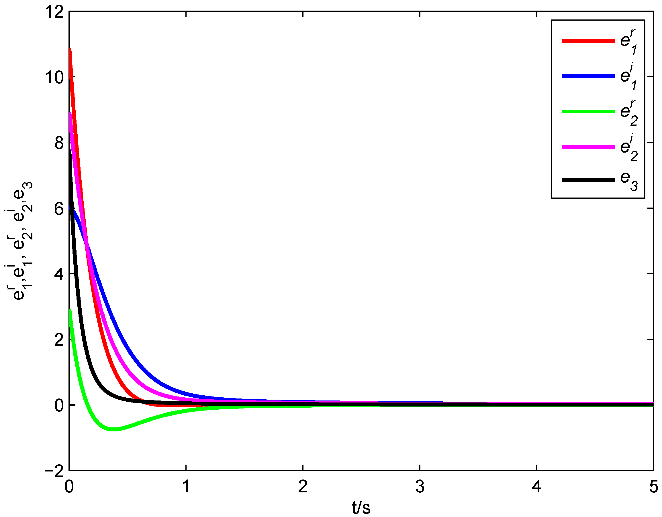
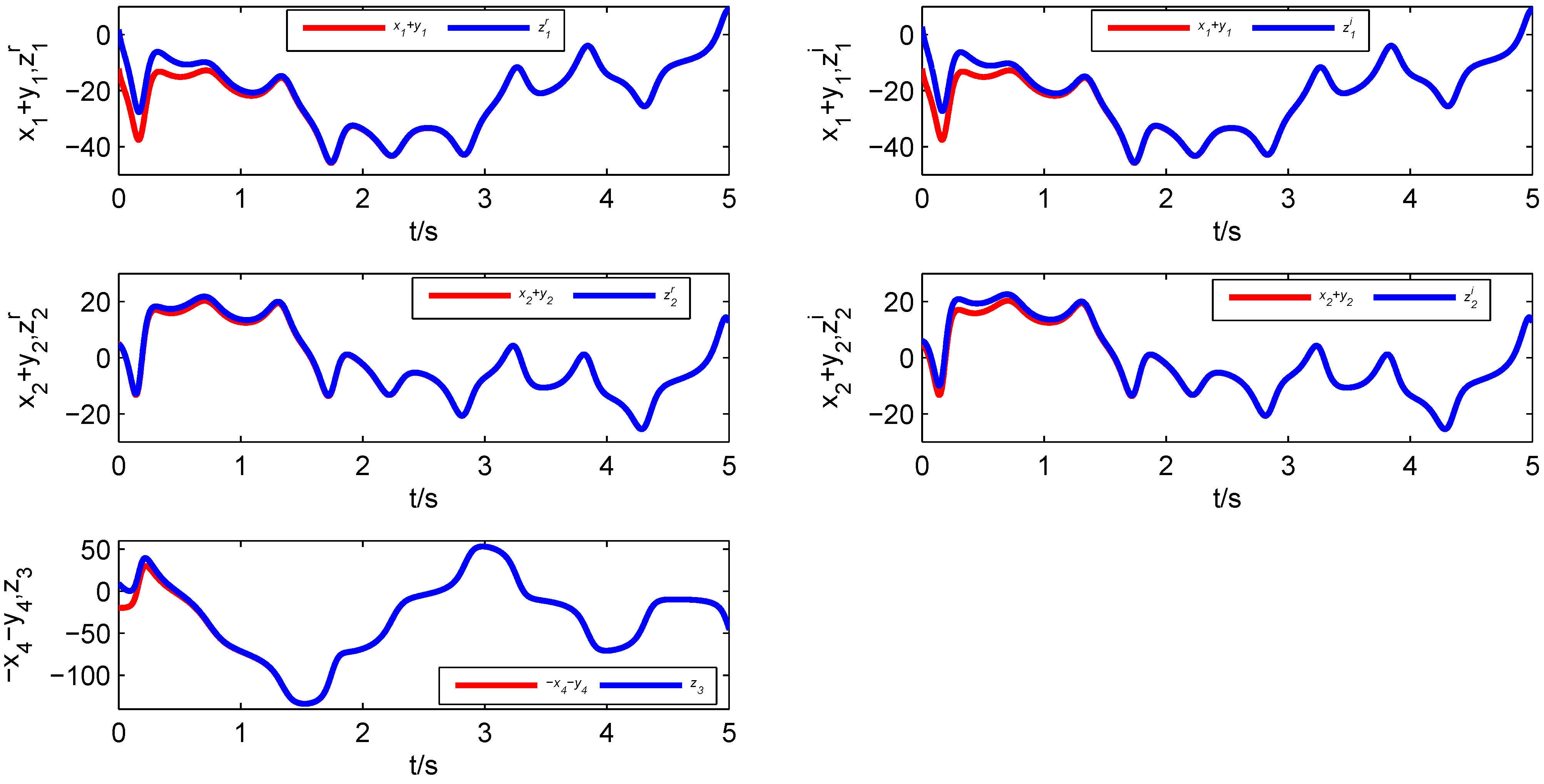
Figure 4, where the red line presents the states of two drive systems and the blue line shows the states of one response system. From 
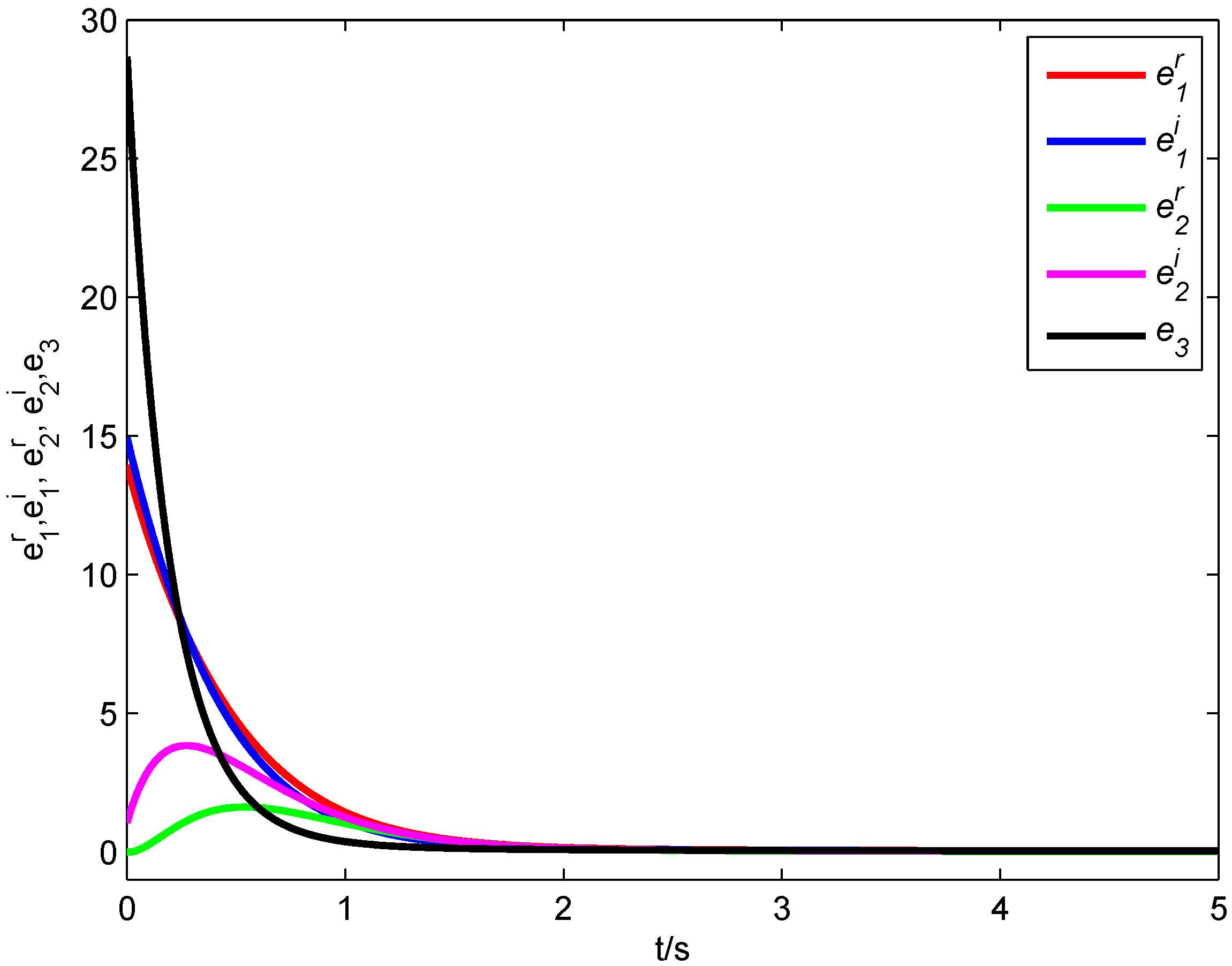
Figure 5, it is clear that all error states converge asymptotically to zero, i.e., the fractional-order complex Lorenz system, the fractional-order complex Lü system and the fractional-order complex Chen system achieve synchronization with the designed controller.
Figure 4. State variables of the fractional-order complex Systems (8)–(10).
Entropy 17 05199 g004
Figure 5. Synchronization errors of the fractional-order complex Systems (8)–(10).
Entropy 17 05199 g005

4.2. Synchronization between Two Fractional-Order Hyperchaotic Real Drive Systems and a Fractional-Order Chaotic Complex Response System

In order to observe generalized combination complex synchronization between two fractional-order hyperchaotic real drive systems and a fractional-order chaotic complex response system, we assume that the fractional-order hyperchaotic real Chen system and the fractional-order hyperchaotic real Rössler system drive the fractional-order chaotic complex Lorenz system. Two drive systems are introduced below:
D * α x 1 ( t ) = a 1 ( x 2 x 1 ) + x 4 , D * α x 2 ( t ) = a 4 x 1 x 1 x 3 + a 3 x 2 , D * α x 3 ( t ) = x 1 x 2 a 2 x 3 , D * α x 4 ( t ) = x 2 x 3 + a 5 x 4 ,
and:
D * α y 1 ( t ) = y 2 y 3 , D * α y 2 ( t ) = y 1 + b 1 y 2 + y 4 , D * α y 3 ( t ) = b 2 + y 1 y 3 , D * α y 4 ( t ) = b 3 y 3 + b 4 y 4 ,
while the response system with the controller is depicted as follows:
D * α z 1 ( t ) = c 1 ( z 2 z 1 ) + U 1 , D * α z 2 ( t ) = c 2 z 1 z 1 z 3 z 2 + U 2 , D * α z 3 ( t ) = 1 2 ( z ¯ 1 z 2 + z 1 z ¯ 2 ) c 3 z 3 + U 3 ,
where A = a 1 a 1 0 1 a 4 a 3 0 0 0 0 a 2 0 0 0 0 a 5 , B = 0 1 1 0 1 b 1 0 1 0 0 0 0 0 0 b 3 b 4 , C = c 1 c 1 0 c 2 1 0 0 0 c 3 , f ( x ) = 0 x 1 x 3 x 1 x 2 x 2 x 3 , g ( y ) = 0 0 b 2 + y 1 y 3 0 , h ( z ) = 0 z 1 z 3 1 2 ( z ¯ 1 z 2 + z 1 z ¯ 2 ) ; z 1 = z 1 r + j z 1 i and z 2 = z 2 r + j z 2 i are complex variables, x i , y i and z 3 are real variables ( i = 1 , 2 , 3 , 4 ) and U 1 = u 1 + j u 2 , U 2 = u 3 + j u 4 and U 3 = u 5 are complex and real control functions, respectively.
For two given scaling matrices D 1 = D 2 = 1 + j 0 0 0 0 1 + j 0 0 0 0 0 1 , the synchronization error is described as follows:
e 1 ( t ) = e 1 r + j e 1 i = z 1 r x 1 y 1 + j ( z 1 i x 1 y 1 ) , e 2 ( t ) = e 2 r + j e 2 i = z 2 r x 2 y 2 + j ( z 2 i x 2 y 2 ) , e 3 ( t ) = z 3 + x 4 + y 4 .
Taking a control matrix as K = 2 c 1 c 1 + 1 0 c 2 2 3 1 0 0 c 3 + 5 , we get C K = 2 1 0 2 4 1 0 0 5 with ( c 1 , c 2 , c 3 ) = ( 10 , 180 , 1 ) . Thus, when α = 0 . 98 , all eigenvalues of C K are λ 1 , 2 = 4 ± 2 j and λ 3 = 10 , which lie in the region | arg ( λ i ( C K ) ) | > α π / 2 ( i = 1 , 2 , 3 ).
From Corollary 1, the control law is obtained as follows:
u 1 = ( c 1 a 1 ) x 1 + c 1 y 1 + ( a 1 c 1 ) x 2 ( c 1 + 1 ) y 2 + x 4 y 3 ( 2 c 1 ) e 1 r ( c 1 + 1 ) e 2 r , u 2 = ( c 1 a 1 ) x 1 + c 1 y 1 + ( a 1 c 1 ) x 2 ( c 1 + 1 ) y 2 + x 4 y 3 ( 2 c 1 ) e 1 i ( c 1 + 1 ) e 2 i , u 3 = ( a 4 c 2 ) x 1 + ( 1 c 2 ) y 1 + ( a 3 + 1 ) x 2 + ( b 1 + 1 ) y 2 + y 4 x 1 x 3 + z 1 r z 3 ( c 2 2 ) e 1 r 3 e 2 r e 3 , u 4 = ( a 4 c 2 ) x 1 + ( 1 c 2 ) y 1 + ( a 3 + 1 ) x 2 + ( b 1 + 1 ) y 2 + y 4 x 1 x 3 + z 1 i z 3 ( c 2 2 ) e 1 i 3 e 2 i , u 5 = ( c 3 + a 5 ) x 4 ( b 4 + c 3 ) y 4 z 1 r z 2 r z 1 i z 2 i x 2 x 3 + b 3 y 3 ( 5 c 3 ) e 3 .
In the following, α = 0 . 98 , the initial values of Systems (11)–(13) are taken as x ( 0 ) = ( 3 , 4 , 2 , 2 ) T , y ( 0 ) = ( 15 , 9 , 4 , 18 ) T , z ( 0 ) = ( 2 + 3 j , 5 + 6 j , 9 ) T , and the parameters are chosen as ( a 1 , a 2 , a 3 , a 4 , a 5 ) = ( 35 , 3 , 12 , 7 , 0 . 5 ) , ( b 1 , b 2 , b 3 , b 4 ) = ( 0 . 25 , 3 , 0 . 5 , 0 . 05 ) , ( c 1 , c 2 , c 3 ) = ( 10 , 180 , 1 ) . Then, Systems (11) and (12) exhibit chaotic attractors, as shown in Figure 6 and Figure 7. 
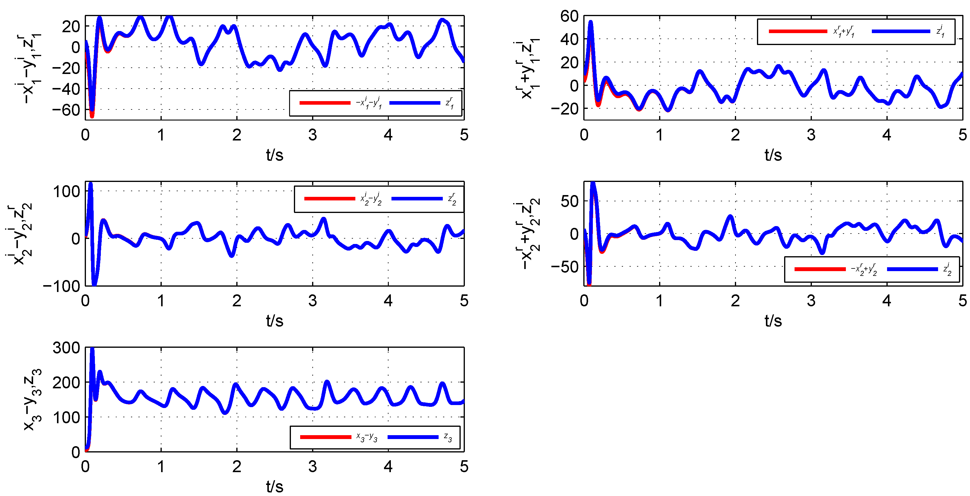
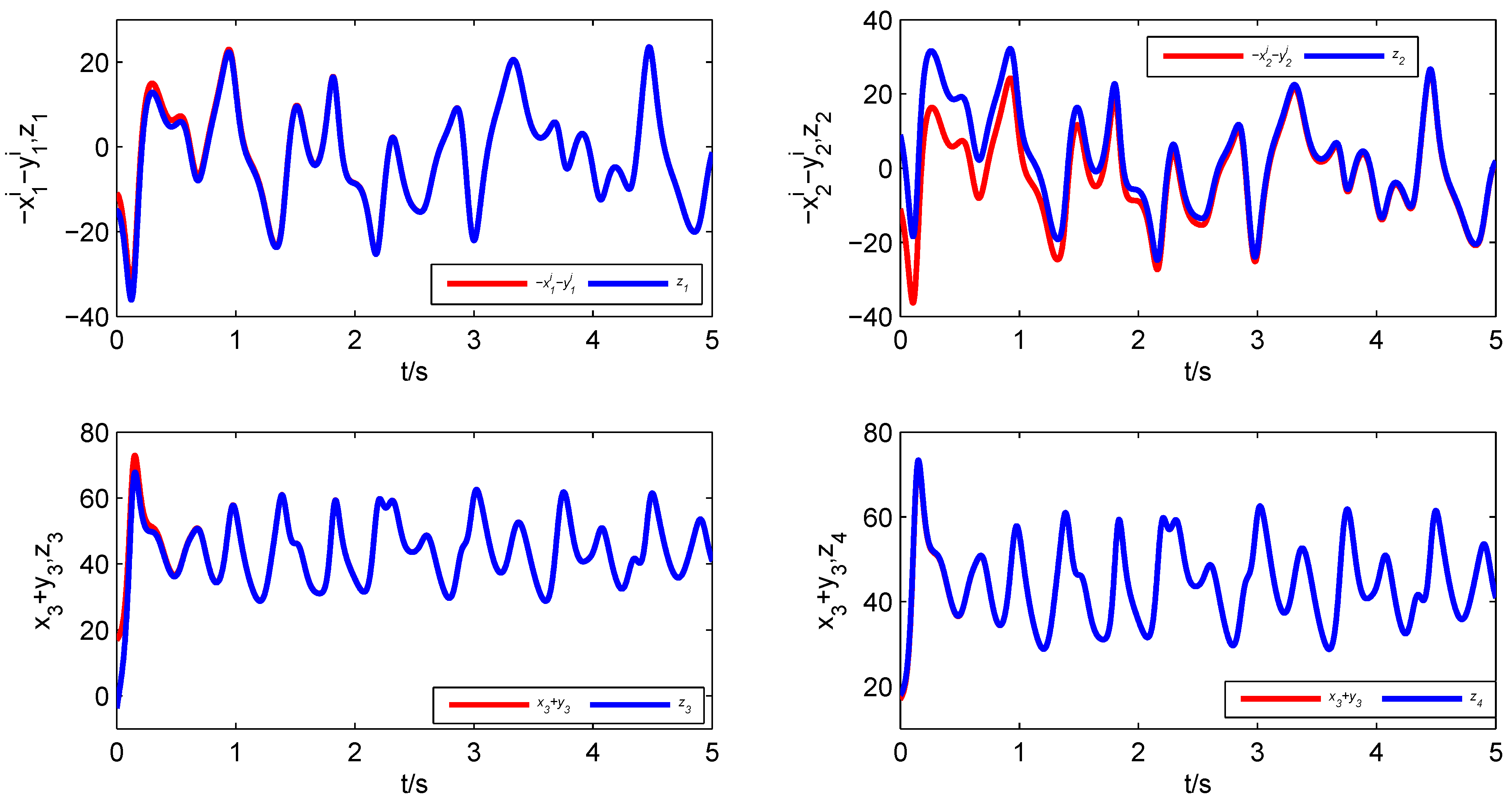
Figure 8 demonstrates the synchronization process and error states of Systems (11)–(13). According to Figure 9, it is obvious that all error states tend asymptotically to zero. Hence, the four-dimensional fractional-order real Chen system, the four-dimensional fractional-order real Rössler system and the three-dimensional fractional-order complex Lorenz system realize generalized combination complex synchronization.
Figure 6. 
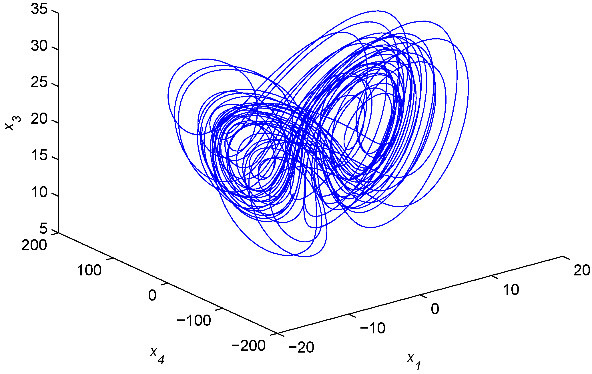
Chaotic attractor of the fractional-order hyperchaotic real Chen system.
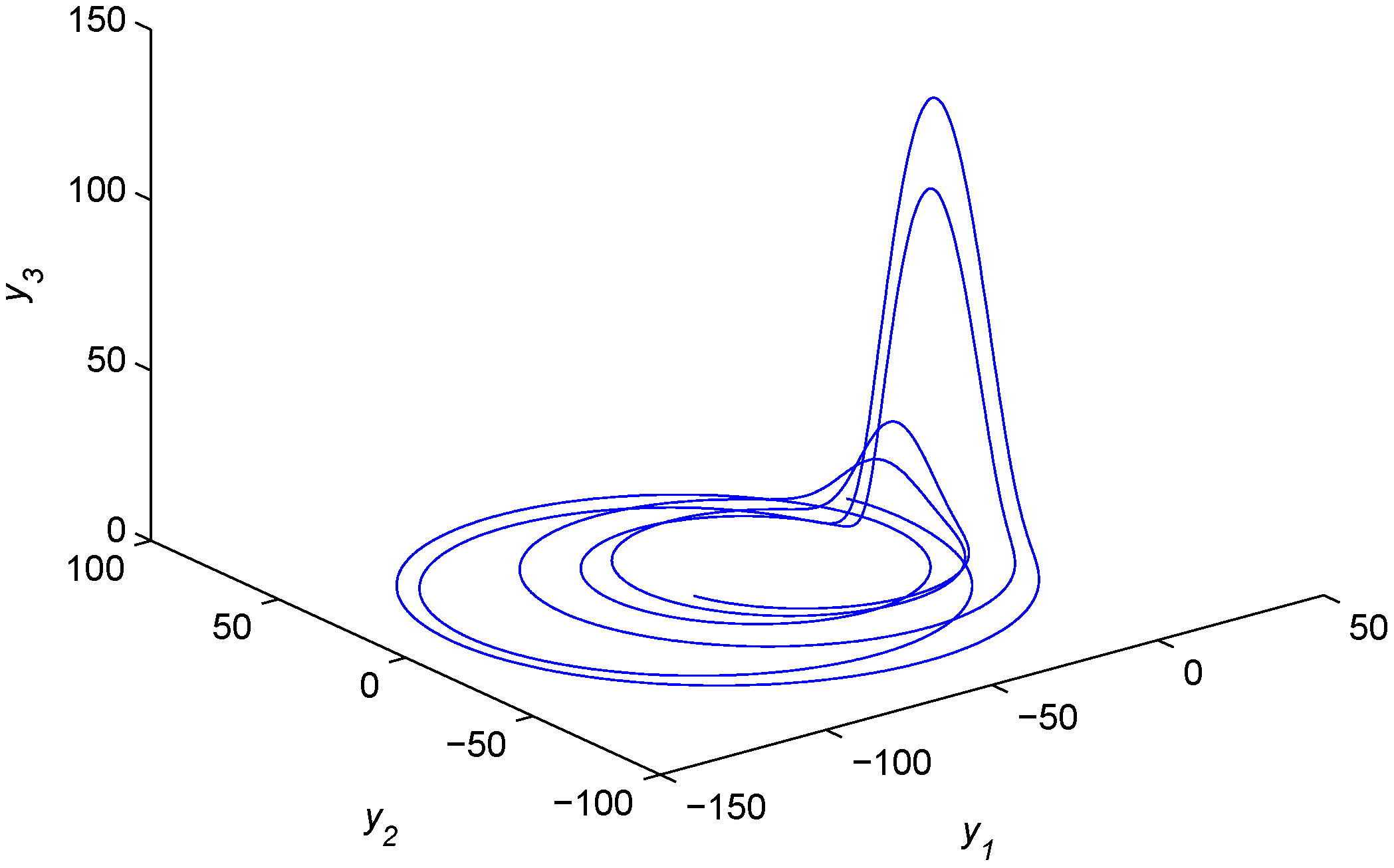
Entropy 17 05199 g006
Figure 7. Chaotic attractor of the fractional-order hyperchaotic real Rössler system.
Entropy 17 05199 g007
Figure 8. State variables of the fractional-order nonlinear Systems (11)–(13).
Entropy 17 05199 g008
Figure 9. Synchronization errors of the fractional-order Systems (11)–(13).
Entropy 17 05199 g009

4.3. Synchronization between Two Fractional-Order Chaotic Complex Drive Systems and a Fractional-Order Hyperchaotic Real Response System

In this subsection, we design the control law to achieve generalized combination complex synchronization between the fractional-order complex Lü system, the fractional-order complex Chen system and the fractional-order hyperchaotic real Rössler system. The first drive system is defined as:
D * α x 1 ( t ) = a 1 ( x 2 x 1 ) , D * α x 2 ( t ) = a 2 x 2 x 1 x 3 , D * α x 3 ( t ) = 1 2 ( x ¯ 1 x 2 + x 1 x ¯ 2 ) a 3 x 3 ,
and the second drive system is given as:
D * α y 1 ( t ) = b 1 ( y 2 y 1 ) , D * α y 2 ( t ) = ( b 2 b 1 ) y 1 + b 2 y 2 y 1 y 3 , D * α y 3 ( t ) = 1 2 ( y ¯ 1 y 2 + y 1 y ¯ 2 ) b 3 y 3 ,
while the response system with the controller is described as follows:
D * α z 1 ( t ) = z 2 z 3 + U 1 , D * α z 2 ( t ) = z 1 + c 1 z 2 + z 4 + U 2 , D * α z 3 ( t ) = c 2 + z 1 z 3 + U 3 , D * α z 4 ( t ) = c 3 z 3 + c 4 z 4 + U 4 ,
where A = a 1 a 1 0 0 a 2 0 0 0 a 3 , B = b 1 b 1 0 b 2 b 1 b 2 0 0 0 b 3 , C = 0 1 1 0 1 c 1 0 1 0 0 0 0 0 0 c 3 c 4 , f ( x ) = 0 x 1 x 3 1 2 ( x ¯ 1 x 2 + x 1 x ¯ 2 ) , g ( y ) = 0 y 1 y 3 1 2 ( y ¯ 1 y 2 + y 1 y ¯ 2 ) , h ( z ) = 0 0 c 2 + z 1 z 3 0 ; x 1 = x 1 r + j x 1 i , x 2 = x 2 r + j x 2 i , y 1 = y 1 r + j y 1 i and y 2 = y 2 r + j y 2 i are complex variables, x 3 , y 3 and z i are real variables and U i are real control functions ( i = 1 , 2 , 3 , 4 ).
Suppose two scaling matrices D 1 = D 2 = j 0 0 0 j 0 0 0 1 0 0 1 = 0 0 0 0 0 0 0 0 1 0 0 1 + j 1 0 0 0 1 0 0 0 0 0 0 0 . The real synchronization error is defined as follows:
e 1 ( t ) = z 1 + x 1 i + y 1 i , e 2 ( t ) = z 2 + x 2 i + y 2 i , e 3 ( t ) = z 3 x 3 y 3 , e 4 ( t ) = z 4 x 3 y 3 .
Select a control matrix as K = λ 1 1 1 0 1 c 1 λ 2 0 1 0 0 λ 3 0 0 0 c 3 c 4 λ 4 , where λ i are real and satisfy | arg ( λ i ( C K ) ) | > α π / 2 , ( i = 1 , 2 , 3 , 4 ) .
The real controller is derived from Corollary 3 as follows:
U 1 = a 1 x 1 i + b 1 y 1 i ( 1 + a 1 ) x 2 i ( 1 + b 1 ) y 2 i + x 3 + y 3 + λ 1 e 1 + e 2 + e 3 , U 2 = x 1 i + y 1 i ( b 2 b 1 ) y 1 i + ( c 1 a 2 ) x 2 i + ( c 1 b 2 ) y 2 i x 3 y 3 + x 1 i x 3 + y 1 i y 3 e 1 ( c 1 λ 2 ) e 2 e 4 , U 3 = c 2 z 1 z 3 + x 1 r x 2 r + x 1 i x 2 i a 3 x 3 b 3 y 3 + y 1 r y 2 r + y 1 i y 2 i + λ 3 e 3 , U 4 = ( c 3 c 4 a 3 ) x 3 + ( c 3 c 4 b 3 ) y 3 + x 1 r x 2 r + x 1 i x 2 i + y 1 r y 2 r + y 1 i y 2 i + c 3 e 3 ( c 4 λ 4 ) e 4 .
In what follows, α = 0 . 98 , the initial values are x ( 0 ) = ( 1 + 2 j , 3 + 4 j , 9 ) T , y ( 0 ) = ( 6 + 9 j , 5 + 7 j , 12 ) T , z ( 0 ) = ( 15 , 9 , 4 , 18 ) T , and the parameters are ( a 1 , a 2 , a 3 ) = ( 42 , 22 , 5 ) , ( b 1 , b 2 , b 3 ) = ( 35 , 28 , 3 ) , ( c 1 , c 2 , c 3 , c 4 ) = ( 0 . 25 , 3 , 0 . 5 , 0 . 05 ) . we choose λ 1 = 2 , λ 2 = 1 , λ 3 = 9 and λ 4 = 5 , such that all eigenvalues of C K lie in region | arg ( λ i ( C K ) ) | > α π / 2 ( i = 1 , 2 , 3 , 4 ). 
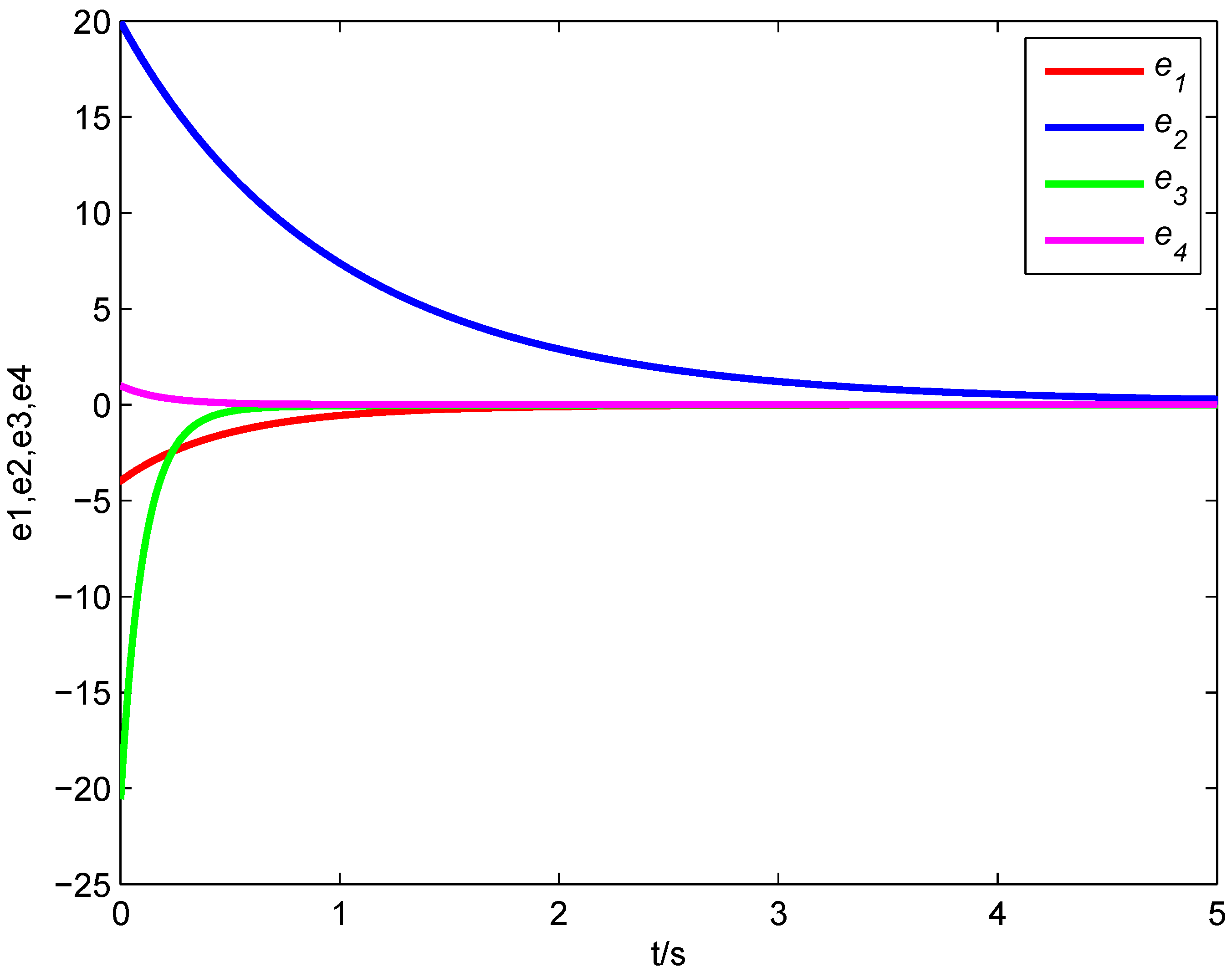
Figure 10 describes the synchronization process of Systems (14)–(16). According to Figure 11, it can be seen that all error states converge asymptotically to zero. Therefore, the fractional-order chaotic complex Lü system, the fractional-order chaotic complex Chen system and the fractional-order hyperchaotic real Rössler achieve generalized combination complex synchronization.
Figure 10. State variables of the fractional-order nonlinear Systems (14)–(16).
Entropy 17 05199 g010
Figure 11. Synchronization errors of the fractional-order Systems (14)–(16).
Entropy 17 05199 g011

5. Conclusions

This paper presents generalized combination complex synchronization between two fractional-order complex drive systems and one fractional-order complex response system with different dimensions. In this proposed scheme, two drive systems and one response system can be synchronized to two complex constant scaling matrices which are non-square matrices. The special cases, such as combination complex synchronization, combination synchronization and complex projective synchronization, are discussed, as well. Based on the stability of fractional-order linear systems, a general controller is obtained to achieve generalized combination complex synchronization among three different dimensional fractional-order chaotic complex systems. Through this scheme, we study generalized combination complex synchronization between fractional-order real chaos and complex chaos. Furthermore, this scheme is successfully applied to three examples. Corresponding simulations verify the feasibility of the proposed scheme. Moreover, the proposed synchronization has advantages over the usual drive-response synchronization, such as being able to provide greater security in secure communication. Therefore, it is believed that the proposed scheme will play an important role in secure communication.

Acknowledgments

The authors would like to thank the editors and anonymous referees for their constructive comments and suggestions. The research was supported by the National Natural Science Foundation of China (Numbers 61273088, 10971120) and the Natural Science Foundation of Shandong Province (Number ZR2010FM010).

Author Contributions

All three authors contributed equally to this work and are listed in alphabetical order. They all read and approved the final version of the manuscript.

Conflicts of Interest

The authors declare no conflict of interest.

References

  1. Sabatier, J.; Agrawal, O.; Tenreiro Machado, J.A. Advances in Fractional Calculus: Theoretical Developments and Application in Physics And Engineering; Springer: Berlin, Germany, 2007. [Google Scholar]
  2. Scalas, E. Applications of continuous-time random walks in finance and economics. Physica A 2006, 362, 225–239. [Google Scholar] [CrossRef]
  3. Lorenzo, C.F.; Hartley, T.T. Initialization of Fractional Differential Equations: Theory and Application. In Proceedings of the ASME 2007 International Design Engineering Technical Conferences, DETC2007-34814, Las Vegas, NV, USA, 4–7 September 2007; pp. 1341–1347.
  4. Hartley, T.T.; Lorenzo, C.F. Dynamics and Control of Initialized Fractional-Order Systems. Nonlinear Dyn. 2002, 29, 201–233. [Google Scholar] [CrossRef]
  5. Du, M.L.; Wang, Z.H. Correcting the initialization of models with fractional derivatives via history-dependent conditions. Acta Mech. Sin. 2015. [Google Scholar] [CrossRef]
  6. Hartley, T.T.; Lorenzo, C.F.; Qammar, H.K. Chaos in a fractional order Chua’s system. IEEE Trans. Circuits Syst. 1995, 42, 485–490. [Google Scholar] [CrossRef]
  7. Wu, X.J.; Lu, Y. Generalized projective synchronization of the fractional-order Chen hyperchaotic system. Nonlinear Dyn. 2009, 57, 25–35. [Google Scholar] [CrossRef]
  8. Li, C.G.; Chen, G.R. Chaos and hyperchaos in the fractional-order Rössler equations. Physica A 2004, 341, 55–61. [Google Scholar] [CrossRef]
  9. Muthukumar, P.; Balasubramaniam, P. Feedback synchronization of the fractional order reverse butterfly-shaped chaotic system and its application to digital cryptography. Nonlinear Dyn. 2013, 74, 1169–1181. [Google Scholar] [CrossRef]
  10. Muthukumar, P.; Balasubramaniam, P.; Ratnavelu, K. Synchronization of a novel fractional order stretch-twist-fold (STF) flow chaotic system and its application to a new authenticated encryption scheme (AES). Nonlinear Dyn. 2014, 77, 1547–1559. [Google Scholar] [CrossRef]
  11. Zhou, P; Huang, K. A new 4-D non-equilibrum fractional-order chaotic system and its circuit implementation. Commun. Nonlinear Sci. Numer. Simulat. 2014, 19, 2005–2011. [Google Scholar]
  12. Muthukumar, P.; Balasubramaniam, P.; Ratnavelu, K. Synchronization and an application of a novel fractional order King Cobra chaotic system. Chaos 2014, 24, 033105. [Google Scholar] [CrossRef] [PubMed]
  13. Muthukumar, P.; Balasubramaniam, P.; Ratnavelu, K. Fast projective synchronization of fractional order chaotic and reverse chaotic systems with its application to an affine cipher using date of birth (DOB). Nonlinear Dyn. 2015, 80, 1883–1897. [Google Scholar] [CrossRef]
  14. Muthukumar, P.; Balasubramaniam, P.; Ratnavelu, K. Theoretical and practical applications of fuzzy fractional integral sliding mode control for fractional-order dynamical system. Nonlinear Dyn. 2015, 80, 249–267. [Google Scholar]
  15. Agrawal, S.K.; Srivastava, M.; Das, S. Synchronization of fractional-order chaotic systems using active control method. Chaos Solitons Fractals 2012, 45, 737–752. [Google Scholar] [CrossRef]
  16. Odibat, Z.M. Synchronization of chaotic fractional-order system via linear control. Int. J. Bifurc. Chaos 2010, 20, 81–97. [Google Scholar] [CrossRef]
  17. Targhvafard, H.; Enjace, G.H. Phase and anti-phase synchronization of fractional-order chaotic systems via active control. Commun. Nonlinear Sci. Numer. Simulat. 2011, 16, 4079–4088. [Google Scholar] [CrossRef]
  18. Si, G.Q.; Sun, Z.Y.; Zhang, Y.B.; Chen, W.Q. Projective synchronization of differentfractional-order chaotic systems with non-identical orders. Nonlinear Anal. Real World Appl. 2012, 13, 1761–1771. [Google Scholar] [CrossRef]
  19. Tavazoei, M.S.; Haeri, M. Synchronization of chaotic fractional-order systems via active sliding mode controller. Physica A 2008, 387, 57–70. [Google Scholar] [CrossRef]
  20. Srivastava, M.; Ansari, S.P.; Agrawal, S.K.; Das, S.; Leung, A.Y.T. Anti-synchronization between identical and non-identical fractional-order chaotic systems using active control method. Nonlinear Dyn. 2014, 76, 905–914. [Google Scholar] [CrossRef]
  21. Luo, C.; Wang, X.Y. Chaos in the fractional-order complex Lorenz system and its synchronization. Nonlinear Dyn. 2013, 71, 241–257. [Google Scholar] [CrossRef]
  22. Luo, C.; Wang, X.Y. Chaos generated from the fractional-order complex Chen system and its application to digital secure communication. Int. J. Mod. Phys. C 2014, 24, 1350025. [Google Scholar] [CrossRef]
  23. Liu, X.J.; Hong, L.; Yang, L.X. Fractional-order complex T system: bifurcations, chaos control, and synchronization. Nonlinear Dyn. 2014, 75, 589–602. [Google Scholar] [CrossRef]
  24. Jiang, C.M.; Liu, S.T.; Luo, C. A new fractional-order chaotic complex system and its antisynchronization. Abstr. Appl. Anal. 2014, 2014. [Google Scholar] [CrossRef]
  25. Liu, J. Complex modified hybrid projective synchronization of different dimensional fractional-order complex chaos and real hyper-chaos. Entropy 2014, 16, 6195–6211. [Google Scholar] [CrossRef]
  26. Luo, R.Z.; Wang, Y.L.; Deng, S.C. Combination synchronization of three classic chaotic systems using active backstepping design. Chaos 2011, 21, e043114. [Google Scholar]
  27. Wu, Z.Y.; Fu, X.C. Combination synchronization of three differnt order nonlinear systems using active backstepping design. Nonlinear Dyn. 2013, 73, 1863–1872. [Google Scholar] [CrossRef]
  28. Zhou, X.B.; Jiang, M.R; Huang, Y.Q. Combination synchronization of three identical or different nonlinear complex chaotic systems. Entopy 2013, 15, 3746–3761. [Google Scholar]
  29. Sun, J.W.; Cui, G.Z.; Wang, Y.F.; Shen, Y. Combination complex synchronization of three chaotic complex systems. Nonlinear Dyn. 2015, 79, 953–965. [Google Scholar] [CrossRef]
  30. Sun, J.W.; Shen, Y.; Zhang, G.D.; Xu, C.J.; Cui, G.Z. Combination-combination synchronization among four identical or different chaotic systems. Nonlinear Dyn. 2013, 73, 1211–1222. [Google Scholar] [CrossRef]
  31. Zhou, X.B.; Jiang, M.R.; Huang, Y.Q. Combination-combination synchronization of four nonlinear complex hyperchaotic systems. Abstr. Appl. Anal. 2014, 2014. [Google Scholar] [CrossRef]
  32. Sun, J.W.; Shen, Y.; Quan, Y.; Xu, C. J.; Cui, G. Z. Compound synchronization for four memristor chaotic oscillator systems and secure communication. Chaos 2014, 23, e013140. [Google Scholar] [CrossRef] [PubMed]
  33. Caputo, M. Linear models of dissipation whose Q is almost frequency independent-II. Geophys. J. Int. 1967, 13, 529–539. [Google Scholar] [CrossRef]
  34. Matignon, D. Stability Results for Fractional Differential Equations with Applications to Control Processing. In Proceedings of CESA 1996 IMACS Multiconference: Computational Engineering in Systems Applications IMACS, Lille, France, 9–12 July 1996; pp. 963–968.
  35. Diethelm, K.; Ford, N.J.; Freed, A.D. A predictor-corrector approch for the numerical solution of fractional differential equations. Nonlinear Dyn. 2002, 29, 3–22. [Google Scholar] [CrossRef]

