
Minimum Error Entropy Algorithms with Sparsity Penalty Constraints


Abstract
:1. Introduction
2. MEE and CIM
2.1. Minimum Error Entropy Criterion
2.2. Correntropy Induced Metric
- Non-negativity: CIM(X, Y) ≥ 0.
- Identity of indiscernible: CIM(X, Y) = 0 if and only if X = Y.
- Symmetry: CIM(X,Y) = CIM(Y,X).
- Triangle inequality: CIM(X,Z)<CIM(X, Y) + CIM(Y,Z).
3. Sparse MEE Algorithms
3.1. Sparse MEE with Zero-Attracting (l1-norm) Penalty Term (ZAMEE)
3.2. Sparse MEE with the Logarithmic Penalty Term (RZAMEE)
3.3. Sparse MEE with CIM Penalty Term (CIMMEE)
4. Mean Square Convergence Analysis
4.1. Energy Conservation Relation
4.2. Sufficient Condition for Mean Square Convergence
- The noise {v(n)} is independent, identically distributed, and independent of the input {X(n)}.
- The a priori error vector is jointly Gaussian distributed.
- The input vectors {X(n)} are zero-mean independent, identically distributed.
- ∀i,j∈{n−L + 1,⋯,n}, ℜi,j (n) is independent of {e(i),e (j)}.
- The vectors {G(W(n))} are zero-mean independent, identically distributed, and independent of the input {X(n)}.
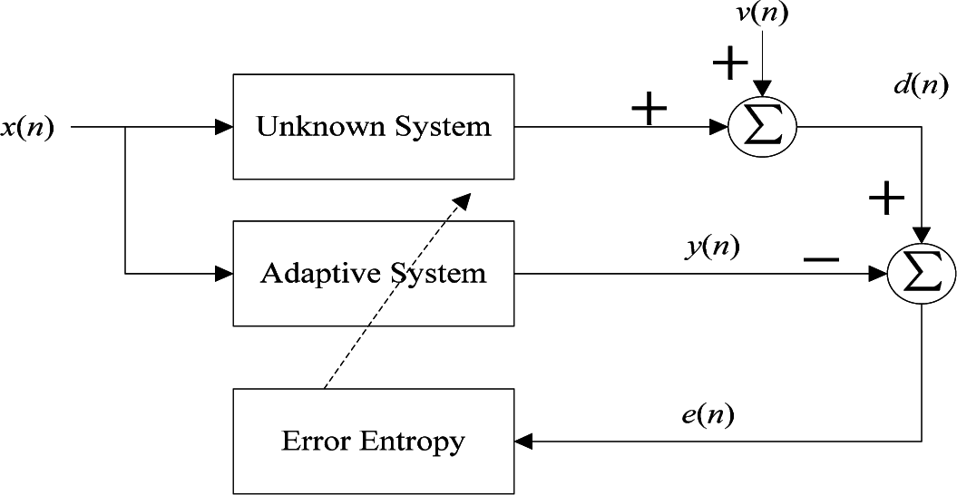
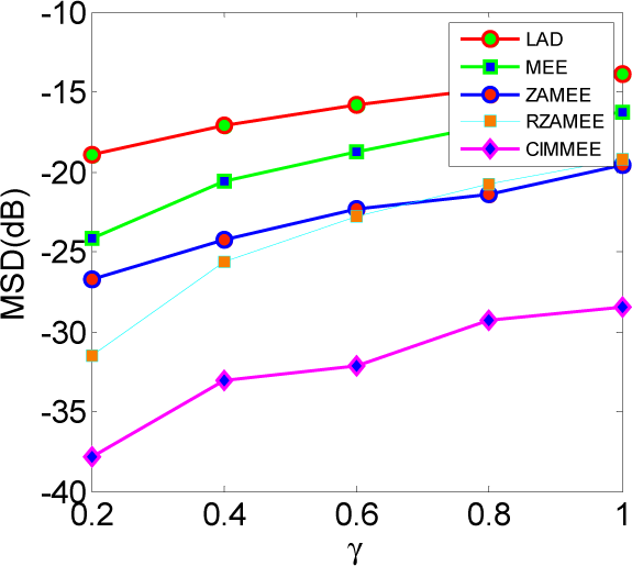
5. Simulation Results
5.1. Experiment 1
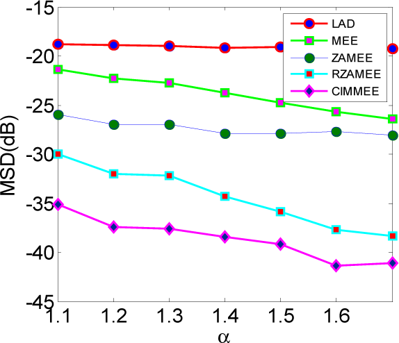
5.2. Experiment 2
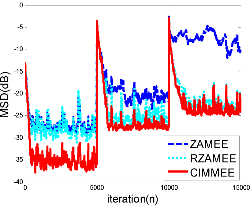
5.3. Experiment 3
6. Conclusion
Acknowledgments
Author Contributions
Conflicts of Interest
References
- Chen, Y.; Gu, Y.; Hero, A.O. Sparse LMS for system identification, Proceedings of 35th IEEE International Conference on Acoustics, Speech and Signal Processing (ICASSP2009), Taipei, Taiwan, 19–24 April 2009; pp. 3125–3128.
- Gu, Y.; Jin, J.; Mei, S. l0 norm constraint LMS algorithm for sparse system identification. IEEE Signal Process. Lett. 2009, 16, 774–777. [Google Scholar]
- Jin, J.; Qu, Q.; Gu, Y. Robust Zero-point Attraction Least Mean Square Algorithm on Near Sparse System Identification. IET Signal Process. 2013, 7, 210–218. [Google Scholar]
- Shi, K.; Shi, P. Convergence analysis of sparse LMS algorithms with l1-norm penalty based on white input signal. Signal Process 2010, 90, 3289–3293. [Google Scholar]
- Yin, D.; So, H.C.; Gu, Y. Sparse Constraint Affine Projection Algorithm with Parallel Implementation and Application in Compressive Sensing, Proceedings of 39th IEEE International Conference on Acoustics, Speech, and Signal Processing (ICASSP2014), Florence, Italy, 4–9 May 2014; pp. 7288–7292.
- Babadi, B.; Kalouptsidis, N.; Tarokh, V. SPARLS: The sparse RLS algorithm. IEEE Trans. Signal Process. 2010, 58, 4013–4025. [Google Scholar]
- Wu, F.Y.; Tong, F. Gradient optimization p-norm-like constraint LMS algorithm for sparse system estimation. Signal Process 2013, 93, 967–971. [Google Scholar]
- Salman, M.S. Sparse leaky LMS algorithm for system identification and its convergence analysis. Int. J. Adapt. Control Signal Process. 2014, 28, 1065–1072. [Google Scholar]
- Aliyu, M.L.; Alkassim, M.A.; Salman, M.S. A p-norm variable step-size LMS algorithm for sparse system identification. Signal Image Video Process 2014. [Google Scholar] [CrossRef]
- Wu, F.Y.; Tong, F. Non-Uniform Norm Constraint LMS Algorithm for Sparse System Identification. IEEE Commun. Lett. 2013, 17, 385–388. [Google Scholar]
- Das, B.K.; Chakraborty, M. Sparse Adaptive Filtering by an Adaptive Convex Combination of the LMS and the ZA-LMS Algorithms. IEEE Trans. Circuits Syst. 2014, 61, 1499–1507. [Google Scholar]
- Liu, Y.; Li, C.; Zhang, Z. Diffusion sparse least-mean squares over networks. IEEE Trans. Signal Process 2012, 60, 4480–4485. [Google Scholar]
- Plataniotis, K.N.; Androutsos, D.; Venetsanopoulos, A.N. Nonlinear filtering of non-Gaussian noise. J. Intell. Robot. Syst. 1997, 19, 207–231. [Google Scholar]
- Weng, B.; Barner, K.E. Nonlinear system identification in impulsive environments. IEEE Trans. Signal Process. 2005, 53, 2588–2594. [Google Scholar]
- Golub, G.H.; van Loan, C.F. Matrix Computation; the Johns Hopkins University Press: Baltimore, MD, USA, 1983. [Google Scholar]
- Principe, J.C. Information Theoretic Learning: Renyi’s Entropy and Kernel Perspectives; Springer: New York, NY, USA, 2010. [Google Scholar]
- Chen, B.; Zhu, Y.; Hu, J.; Principe, J.C. System Parameter Identification: Information Criteria and Algorithms; Elsevier: Amsterdam, The Netherlands, 2013. [Google Scholar]
- Erdogmus, D.; Principe, J.C. From linear adaptive filtering to nonlinear information processing. IEEE Signal Process. Mag. 2006, 23, 15–33. [Google Scholar]
- Erdogmus, D.; Principe, J.C. An error-entropy minimization for supervised training of nonlinear adaptive systems. IEEE Trans. Signal Process. 2002, 50, 1780–1786. [Google Scholar]
- Chen, B.; Hu, J.; Pu, L.; Sun, Z. Stochastic gradient algorithm under (h, ϕ)-entropy criterion. Circuit Syst. Signal Process 2007, 26, 941–960. [Google Scholar]
- Wolsztynski, E.; Thierry, E.; Pronzato, L. Minimum-entropy estimation in semi-parametric models. Signal Process. 2005, 85, 937–949. [Google Scholar]
- Song, A.; Qiu, T. The Equivalency of Minimum Error Entropy Criterion and Minimum Dispersion Criterion for Symmetric Stable Signal Processing. IEEE Signal Process. Lett. 2010, 17, 32–35. [Google Scholar]
- Chen, B.; Principe, J.C. Some further results on the minimum error entropy estimation. Entropy 2012, 14, 966–977. [Google Scholar]
- Chen, B.; Zhu, Y.; Hu, J. Mean-square convergence analysis of ADALINE training with minimum error entropy criterion. IEEE Trans. Neural Netw. 2010, 21, 1168–1179. [Google Scholar]
- Chen, B.; Principe, J.C. On the Smoothed Minimum Error Entropy Criterion. Entropy 2012, 14, 2311–2323. [Google Scholar]
- Li, C.; Shen, P.; Liu, Y.; Zhang, Z. Diffusion information theoretic learning for distributed estimation over network. IEEE Trans. Signal Process. 2013, 61, 4011–4024. [Google Scholar]
- Xue, Y.; Zhu, X. The minimum error entropy based robust wireless channel tracking in impulsive noise. IEEE Commun. Lett. 2002, 6, 228–230. [Google Scholar]
- Liu, W.F.; Pokharel, P.P.; Principe, J.C. Correntropy: Properties and Applications in Non-Gaussian Signal Processing. IEEE Trans. Signal Process. 2007, 55, 5286–5298. [Google Scholar]
- Seth, S.; Principe, J.C. Compressed signal reconstruction using the correntropy induced metric, Proceedings of IEEE International Conference on Acoustics, Speech, and Signal Processing (ICASSP2008), Las Vegas, NV, USA, 31 March–4 April 2008; pp. 3845–3848.
- Wipf, D.P.; Nagarajan, S.S. A new view of automatic relevance determination. Adv. Neural Inf. Process. Syst. 2008. Available online: http://papers.nips.cc/paper/3372-a-new-view-of-automatic-relevance-determination accessed on 5 May 2015.
- Chen, B.; Zhu, P.; Principe, J.C. Survival information potential: A new criterion for adaptive system training. IEEE Trans. Signal Process. 2012, 60, 1184–1194. [Google Scholar]
- Principe, J.C.; Xu, D.; Zhao, Q.; John, F. Learning from examples with information theoretic criteria. J.VLSI Signal Process. Syst. Signal Image Video Technol. 2000, 26, 61–77. [Google Scholar]
- Chen, B.; Xing, L.; Liang, J.; Zheng, N.; Principe, J.C. Steady-state Mean-square Error Analysis for Adaptive Filtering under the Maximum Correntropy Criterion. IEEE Signal Process. Lett. 2014, 21, 880–884. [Google Scholar]
- Chen, B.; Principe, J.C. Maximum correntropy estimation is a smoothed MAP estimation. IEEE Signal Process. Lett. 2012, 19, 491–494. [Google Scholar]
- Al-Naffouri, T.Y.; Sayed, A.H. Adaptive filters with error nonlinearities: Mean-square analysis and optimum design. EURASIP J. Appl. Signal Process. 2001, 4, 192–205. [Google Scholar]
- Douglas, S.C.; Meng, T.H.Y. Stochastic gradient adaptation under general error criteria. IEEE Trans. Signal Process. 1994, 42, 1335–1351. [Google Scholar]
- Sayed, A.H. Fundamentals of Adaptive Filtering; Wiley: New York, NY, USA, 2003. [Google Scholar]
- Shin, H.-C.; Sayed, A.H. Mean-square performance of a family of affine projection algorithms. IEEE Trans. Signal Process. 2004, 52, 90–102. [Google Scholar]
- Papoulis, E.V.; Stathaki, T. A normalized robust mixed-norm adaptive algorithm for system identification. Signal Process. Lett. 2004, 11, 5286–5298. [Google Scholar]
- Shao, M.; Nikias, C.L. Signal processing with fractional lower order moments: Stable processes and their applications. Proc. IEEE 1993, 81, 986–1010. [Google Scholar]
- Weng, B.; Barner, K.E. Nonlinear system identification in impulsive environments. IEEE Trans. Signal Process. 2005, 53, 2588–2594. [Google Scholar]
- Georgiadis, A.T.; Mulgrew, B. A family of recursive algorithms for channel identification in alpha-stable noise, Proceedings of the Fifth Bayona Workshop on Emerging Technologies in Telecommunications, Bayona, Spain, 6–8 September 1999; pp. 153–157.
- Wang, J.; Kuruoglu, E.E.; Zhou, T. Alpha-stable channel capacity. IEEE Commun. Lett. 2011, 15, 1107–1109. [Google Scholar]


© 2015 by the authors; licensee MDPI, Basel, Switzerland This article is an open access article distributed under the terms and conditions of the Creative Commons Attribution license (http://creativecommons.org/licenses/by/4.0/).
Share and Cite
Wu, Z.; Peng, S.; Ma, W.; Chen, B.; Principe, J.C. Minimum Error Entropy Algorithms with Sparsity Penalty Constraints. Entropy 2015, 17, 3419-3437. https://doi.org/10.3390/e17053419
Wu Z, Peng S, Ma W, Chen B, Principe JC. Minimum Error Entropy Algorithms with Sparsity Penalty Constraints. Entropy. 2015; 17(5):3419-3437. https://doi.org/10.3390/e17053419
Chicago/Turabian StyleWu, Zongze, Siyuan Peng, Wentao Ma, Badong Chen, and Jose C. Principe. 2015. "Minimum Error Entropy Algorithms with Sparsity Penalty Constraints" Entropy 17, no. 5: 3419-3437. https://doi.org/10.3390/e17053419
APA StyleWu, Z., Peng, S., Ma, W., Chen, B., & Principe, J. C. (2015). Minimum Error Entropy Algorithms with Sparsity Penalty Constraints. Entropy, 17(5), 3419-3437. https://doi.org/10.3390/e17053419