A Novel Approach to Canonical Divergences within Information Geometry

Abstract

A divergence function on a manifold M defines a Riemannian metric g and dually coupled affine connections ∇ and ${\nabla }^{*}$ on M. When M is dually flat, that is flat with respect to ∇ and ${\nabla }^{*}$, a canonical divergence is known, which is uniquely determined from $(M,g,\nabla ,{\nabla }^{*})$. We propose a natural definition of a canonical divergence for a general, not necessarily flat, M by using the geodesic integration of the inverse exponential map. The new definition of a canonical divergence reduces to the known canonical divergence in the case of dual flatness. Finally, we show that the integrability of the inverse exponential map implies the geodesic projection property.

1. Introduction: Divergence and Dual Geometry

A divergence function $D(p\parallel q)$ is a differentiable real-valued function of two points p and q in a manifold M. It satisfies the non-negativity condition

$$D(p\parallel q)\ge 0$$

(1)

with equality if and only if $p=q$. Thus, it is a distance-like function, but does not necessarily share all properties of a distance. For instance, it can be asymmetric in p and q. When a coordinate system $\mathit{\xi }:p\mapsto {\mathit{\xi }}_p=({\xi }_p^1,\cdots ,{\xi }_p^n)\in {\mathbb{R}}^n$ is given in M, we pose one condition that, for two nearby points ${\mathit{\xi }}_p$ and ${\mathit{\xi }}_q={\mathit{\xi }}_p+\Delta \mathit{\xi }$, D is expanded as

$$D(p\parallel q)=\frac{1}{2}{\stackrel{D}{g}}_{ij}\left(p\right)\Delta {\xi }^i\Delta {\xi }^j+O\left({\parallel \Delta \mathit{\xi }\parallel }^3\right)$$

(2)

and ${({\stackrel{D}{g}}_{ij}\left(p\right))}_{ij}$ is a positive definite matrix. Here, the Einstein summation convention is used, which means that summation is taken with respect to any index that appears twice in a term, as a lower as well as an upper index. Throughout the paper, we apply this convention or explicitly use the summation sign. The coefficients ${\stackrel{D}{g}}_{ij}$ in Equation (2) define a Riemannian metric $\stackrel{D}{g}$. Furthermore, the divergence function D allows us to define also a pair of dual affine connections [1]. In order to be more explicit, we consider coordinates ${\mathit{\xi }}_p=({\xi }_p^1,\cdots ,{\xi }_p^n)$ of p and coordinates ${\mathit{\xi }}_q=({\xi }_q^1,\cdots ,{\xi }_q^n)$ of q and introduce the following simplified notations of differentiation

$${\partial }_i=\frac{\partial }{\partial {\xi }_p^i},{\partial }_i^{\prime }=\frac{\partial }{\partial {\xi }_q^i}$$

(3)

With $D({\mathit{\xi }}_p\parallel {\mathit{\xi }}_q)=D(p\parallel q)$, the coefficients of the Riemannian metric can be written as

$${\stackrel{D}{g}}_{ij}\left(p\right)={\left.-{\partial }_i{\partial }_j^{\prime }D({\mathit{\xi }}_p\parallel {\mathit{\xi }}_q)\right|}_{q=p}={\left.{\partial }_i^{\prime }{\partial }_j^{\prime }D({\mathit{\xi }}_p\parallel {\mathit{\xi }}_q)\right|}_{q=p}$$

(4)

Furthermore, the coefficients

$$\begin{array}{ccc}\hfill {\stackrel{D}{\Gamma }}_{ijk}\left(p\right)& =& {\left.-{\partial }_i{\partial }_j{\partial }_k^{\prime }D({\mathit{\xi }}_p\parallel {\mathit{\xi }}_q)\right|}_{q=p}\hfill \end{array}$$

(5)

$$\begin{array}{ccc}\hfill {\stackrel{D}{{\Gamma }^{*}}}_{ijk}\left(p\right)& =& {\left.-{\partial }_i^{\prime }{\partial }_j^{\prime }{\partial }_{k}D({\mathit{\xi }}_p\parallel {\mathit{\xi }}_q)\right|}_{q=p}\hfill \end{array}$$

(6)

define a pair of dual affine connections $\stackrel{D}{\nabla }$ and $\stackrel{D}{{\nabla }^{*}}$ [1]. The duality of the connections holds with respect to the Riemannian metric $\stackrel{D}{g}$ in terms of the following condition:

$$X\langle Y,Z\rangle =\langle {\stackrel{D}{\nabla }}_{X}Y,Z\rangle +\langle Y,{\stackrel{D}{{\nabla }^{*}}}_{X}Z\rangle$$

(7)

for all vector fields $X,Y$ and Z, where the brackets $\langle ·,·\rangle$ denote the inner product with respect to $\stackrel{D}{g}$ [2].

The inverse problem is to find a divergence D which generates a given geometrical structure $(M,g,\nabla ,{\nabla }^{*})$. Matumoto [3] showed that a divergence exists for any such manifold. However, it is not unique and there are infinitely many divergences that give the same geometrical structure. When a manifold is dually flat, a canonical divergence was introduced by Amari and Nagaoka [2], which is a Bregman divergence. Extensions of the canonical divergence within conformal geometry have been studied by Kurose [4] and Matsuzoe [5]. The canonical divergence has nice properties such as the generalized Pythagorean theorem and the geodesic projection theorem. It is an important problem to define a canonical divergence in the general case. The present paper gives an answer to this problem by using the inverse exponential map. We already used the inverse exponential map in our previous work [6], where we studied a different divergence function. We could show that it recovers the metric g in the sense of Equation (4) and has some consistency with the dual connections ∇ and ${\nabla }^{*}$. However, it turns out that it does not reduce to the well-established canonical divergence in the dually flat case. The divergence introduced in the present article not only recovers the original geometry directly in terms of Equations (4)–(6), it also coincides with the original canonical divergence in the dually flat case.

2. A New Approach to the General Inverse Problem

We begin with a motivation in terms of a simple example where the manifold is ${\mathbb{R}}^n$ equipped with the standard Euclidean metric and connection (here, the Levi-Civita connection): Let p be a fixed point in ${\mathbb{R}}^n$, and consider the vector field pointing to p, that is

$${\mathbb{R}}^n\to {\mathbb{R}}^n,q\mapsto p-q$$

(8)

Obviously, the vector field Equation (8) can be seen as the negative gradient of the squared distance

$$D_p:{\mathbb{R}}^n\to \mathbb{R},q\mapsto D_p\left(q\right):=D(p\parallel q):=\frac{1}{2}{\parallel p-q\parallel }^2=\frac{1}{2}\sum _{i=1}^n{(p_i-q_i)}^2$$

as potential function, that is

$$p-q=-{\text{grad}}_q{D}_p$$

(9)

Here, the gradient ${\text{grad}}_q$ is taken with respect to the canonical inner product on ${\mathbb{R}}^n$.

We shall now generalize the relation Equation (9) between the squared distance $D_p$ and the difference of two points p and q to the more general setting of a differentiable manifold M. Given a fixed point $p\in M$, we want to define a vector field $q\mapsto X(q,p)$, at least in a neighbourhood of p, that corresponds to the difference vector field Equation (8). Obviously, the problem is that the difference $p-q$ is not naturally defined for a general manifold M. We need an affine connection ∇ in order to have a notion of a difference. Given such a connection ∇, for each point $q\in M$ and each direction $X\in T_{q}M$ we consider the geodesic ${\gamma }_{q,X}\left(t\right)$, with the initial point q and the initial velocity X, that is ${\gamma }_{q,X}\left(0\right)=q$ and ${\dot{\gamma }}_{q,X}\left(0\right)=X$. If ${\gamma }_{q,X}\left(t\right)$ is defined for all $0\le t\le 1$, the endpoint $p={\gamma }_{q,X}\left(1\right)$ is interpreted as the result of a translation of the point q along a straight line in the direction of the vector X. This straightness is expressed in terms of the local coordinates $\mathit{\xi }\left(t\right):=({\xi }^1\left(t\right),\cdots ,{\xi }^n\left(t\right)):=\mathit{\xi }\left({\gamma }_{q,X}\left(t\right)\right)$ of the geodesic ${\gamma }_{q,X}$ by the following set of differential equations:

$${\ddot{\xi }}^i\left(t\right)+{\Gamma }_{jk}^i\left(\mathit{\xi }\left(t\right)\right){\dot{\xi }}^j\left(t\right){\dot{\xi }}^k\left(t\right)=0,i=1,\cdots ,n$$

(10)

The translation of points along geodesics defines a map, the so-called exponential map:

$${exp}_q:U_q\to M,X\mapsto {\gamma }_{q,X}\left(1\right)$$

(11)

where $U_q\subseteq T_{q}M$ denotes the set of tangent vectors X, for which the domain of ${\gamma }_{q,X}$ contains the unit interval $[0,1]$.

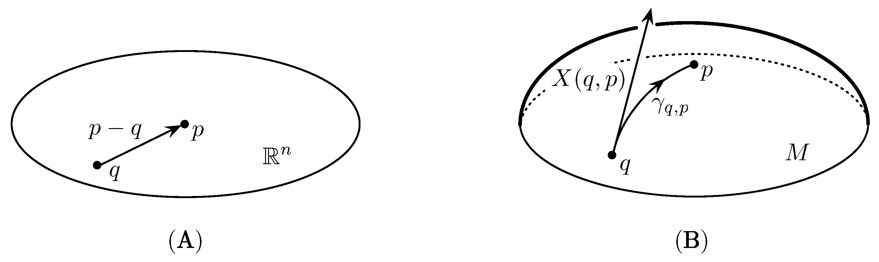
Given two points p and q, one can interpret any X with ${exp}_q\left(X\right)=p$ as a difference vector X that translates q to p. Throughout this paper we assume the existence and uniqueness of such a difference vector, denoted by $X(q,p)$ (see Figure 1).

Figure 1. Illustration of (A) the difference vector $p-q$ in ${\mathbb{R}}^n$ pointing from q to p; and (B) the difference vector $X(q,p)={\dot{\gamma }}_{q,p}\left(0\right)$ as the inverse of the exponential map in q.

Figure 1. Illustration of (A) the difference vector $p-q$ in ${\mathbb{R}}^n$ pointing from q to p; and (B) the difference vector $X(q,p)={\dot{\gamma }}_{q,p}\left(0\right)$ as the inverse of the exponential map in q.

This is a strong assumption, which is, however, always locally satisfied. On one hand, we are mainly interested in local properties. On the other hand, although being quite restrictive in general, this property will be satisfied in our information-geometric context, where g is given by the Fisher metric and ∇ is given by the m- and e-connections and their convex combinations, the α-connections.

If we attach to each point $q\in M$ the difference vector $X(q,p)$, we obtain a vector field that corresponds to the vector field Equation (8) in ${\mathbb{R}}^n$. In order to interpret this vector field as a negative gradient field of a (squared) distance function, and thereby generalize Equation (9), we need a Riemannian metric g on M. Given such a metric, we assume integrability of X and ∇, respectively, in the sense that for all p there exists a function $D_p$ satisfying

$$X(q,p)=-{\text{grad}}_q{D}_p$$

(12)

Here, the Riemannian gradient is taken with respect to g, which is defined by the property that the total differential $d_q{D}_p$ can be expressed as an inner product:

$$\langle {\text{grad}}_q{D}_p,Y\rangle =d_q{D}_p\left(Y\right),Y\in T_{q}M$$

Obviously, if there are functions $D_p$ satisfying the condition of Equation (12) then they are unique up to a constant that can vary with p, and we can therefore assume $D_p\left(p\right)=0$. Throughout the paper we will also use the standard notation $D(p\parallel q)=D_p\left(q\right)$ of a divergence as a function D of two arguments. In order to recover D from Equation (12) we consider any curve $\gamma :[0,1]\to M$ that connects q with p, that is $\gamma \left(0\right)=q$ and $\gamma \left(1\right)=p$. We compose the inner product of the curve velocity $\dot{\gamma }\left(t\right)$ with the inverse of the exponential map $X\left(\gamma \right(t),p)$ in $\gamma \left(t\right)$ and integrate this along the curve:

$$\begin{array}{ccc}\hfill {\int }_0^1\langle X(\gamma \left(t\right),p),\dot{\gamma }\left(t\right)\rangle dt& =& -{\int }_0^1〈{\text{grad}}_{\gamma \left(t\right)}{D}_p,\dot{\gamma }\left(t\right)〉dt\hfill \\ & =& -{\int }_0^1\left(d_{\gamma \left(t\right)}{D}_p\right)\left(\dot{\gamma }\left(t\right)\right)dt\hfill \\ & =& -{\int }_0^1\frac{d{D}_p\circ \gamma }{dt}\left(t\right)dt\hfill \\ & =& D_p\left(\gamma \left(0\right)\right)-D_p\left(\gamma \left(1\right)\right)\hfill \\ & =& D_p\left(q\right)-D_p\left(p\right)=D_p\left(q\right)=D(p\parallel q)\hfill \end{array}$$

(13)

In particular, we can apply this derivation to the geodesic connecting q and p even when the integrability of X is not guaranteed and obtain the definition of a general canonical divergence, discussed in more detail in Section 5. Before we treat the general definition of a canonical divergence, however, we discuss important special cases of divergences within the cone of positive measures and the simplex of probability measures included in it. In particular, we verify that the well-known relative entropy (KL-divergence) and the α-entropy (α-divergence) can be derived in terms of Equation (13).

3. Natural Connections for Positive and Probability Measures

3.1. The Fisher Metric and Its Gradients

We represent measures on the set $\{1,\cdots ,n\}$ as elements of ${\mathbb{R}}^n$. In this representation, the Dirac measures ${\delta }_i$, $i=1,\cdots ,n$, form the canonical basis of ${\mathbb{R}}^n$. We consider the n-dimensional cone of positive measures on the set $\{1,\cdots ,n\}$, defined by

$$M_n:={\mathbb{R}}_{+}^n=\left\{p=\sum _{i=1}^n{p}_i{\delta }_i\in {\mathbb{R}}^n:p_i>0\text{ for all }i\right\}$$

and the corresponding $(n-1)$-dimensional simplex of normalized measures (probability measures) $S_{n-1}\subset M_n$:

$$S_{n-1}:=\left\{p=\sum _{i=1}^n{p}_i{\delta }_i\in {\mathbb{R}}^n:p_i>0\text{ for all }i,\text{ and }{\sum }_{i=1}^n p_i=1\right\}$$

There is a natural Riemannian metric on $M_n$, called the Fisher metric:

$$g_p(X,Y):=\sum _{i=1}^n\frac{1}{p_i}{X}_i{Y}_i,X,Y\in T_p{M}_n$$

In theoretical biology, the Fisher metric is also known as Shahshahani metric (see [7], Equation (7.48)). Given a point $p\in S_{n-1}$ and a vector $X\in T_p{M}_n$, its projection onto $T_p{S}_{n-1}$ with respect to $g_p$ is given by

$${\Pi }_p^{\top }X=\sum _{i=1}^n\left(X_i-p_i\sum _{j=1}^n{X}_j\right){\delta }_i$$

(14)

and the corresponding projection onto the orthogonal complement of $T_p{S}_{n-1}$ is given by

$${\Pi }_p^{\perp }X=\sum _{i=1}^n\left(p_i\sum _{j=1}^n{X}_j\right){\delta }_i$$

(15)

For a function $V:M_n\to \mathbb{R}$, this metric implies the Riemannian gradient

$${\text{grad}}_{p}V=\sum _{i=1}^n\left(p_i\frac{\partial V}{\partial p_i}\left(p\right)\right){\delta }_i$$

(16)

A vector field

$$X_p=\sum _{i=1}^n{p}_i{f}_i\left(p\right){\delta }_i,p\in M_n$$

(17)

is the gradient of a function V if and only if it satisfies for all $i,j$

$$\frac{\partial f_i}{\partial p_j}=\frac{\partial f_j}{\partial p_i}$$

(18)

If we consider a function that is defined on $S_{n-1}$, for instance the restriction of V: $M_n\to \mathbb{R}$ to $S_{n-1}$, then the vector Equation (16), evaluated in $p\in S_{n-1}$, will not necessarily be an element of $T_p{S}_{n-1}$. Therefore, in order to evaluate the gradient on $S_{n-1}$, we have to project the vector Equation (16) onto $T_p{S}_{n-1}$ with respect to the metric g by using Equation (14). This leads to the following gradient formula for functions on $S_{n-1}$:

$${\text{grad}}_{p}V=\sum _{i=1}^n{p}_i\left(\frac{\partial V}{\partial p_i}\left(p\right)-\sum _{j=1}^n{p}_j\frac{\partial V}{\partial p_j}\left(p\right)\right){\delta }_i,p\in S_{n-1}$$

(19)

This gives rise to consider general vector fields of the form

$$X_p=\sum _{i=1}^n{p}_i\left(f_i\left(p\right)-\sum _{j=1}^n{p}_j{f}_j\left(p\right)\right){\delta }_i,p\in S_{n-1}$$

(20)

Such a vector field is integrable, in the sense that it is the gradient Equation (19) of a potential function V, if and only if the following condition holds for all $i,j,k$ (see [7], Equation (19.23)):

$$\frac{\partial f_i}{\partial p_j}+\frac{\partial f_j}{\partial p_k}+\frac{\partial f_k}{\partial p_i}=\frac{\partial f_i}{\partial p_k}+\frac{\partial f_k}{\partial p_j}+\frac{\partial f_j}{\partial p_i}$$

(21)

3.2. The Mixture and the Exponential Connections

After having introduced the Fisher metric and corresponding gradient fields, we now define natural notions of straight lines on $M_n$ and $S_{n-1}$, respectively, induced by corresponding affine connections. Let us first introduce the straight lines of the so-called mixture connection ${\nabla }^{\left(m\right)}$ on $M_n$. Given a point $p\in M_n$ and a direction $X\in T_p{M}_n$, the most natural way to define a straight line that starts in p and has velocity X is given by the so-called m-geodesic

$$\gamma \left(t\right)=p+tX$$

(22)

We obtain the exponential map for $t=1$, which is, in this simple example, the translation:

$${exp}_p^{\left(m\right)}\left(X\right)=p+X$$

The inverse, therefore, maps a point q to the difference vector that translates p into q:

$$X^{\left(m\right)}(p,q):={\left({exp}_p^{\left(m\right)}\right)}^{-1}\left(q\right)=q-p$$

With this difference as X in Equation (22), we obtain the geodesics that connects p with q:

$$\gamma \left(t\right)=p+t(q-p)$$

(23)

If we choose a point $p\in S_{n-1}$ and $X\in T_p{S}_{n-1}$, or two points $p,q\in S_{n-1}$, respectively, then the corresponding geodesic Equation (22) and Equation (23) will stay in $S_{n-1}$. Therefore, the restriction of the exponential map to $T_p{S}_{n-1}$ and its inverse are trivial:

$${\overline{exp}}_p^{\left(m\right)}\left(X\right)=p+X,\overline{X}(p,q):={\left({\overline{exp}}_p^{\left(m\right)}\right)}^{-1}\left(q\right)=q-p$$

where we use a bar over symbols in order to denote the restriction of corresponding objects to $S_{n-1}$.

Now let us come to the notion of an e-geodesic and the exponential map of the so-called e-connection ${\nabla }^{\left(e\right)}$. Given a point $p\in M_n$ and a direction $X\in T_p{M}_n$, we consider the geodesic

$$\gamma \left(t\right)=\sum _{i=1}^n{p}_{i}exp\left(t\frac{X_i}{p_i}\right){\delta }_i$$

(24)

(The “exp” on the right-hand side of Equation (24) denotes the standard real-valued natural exponential function.) The exponential map of the e-connection is given for $t=1$:

$${exp}_p^{\left(e\right)}\left(X\right)=\sum _{i=1}^n{p}_{i}exp\left(\frac{X_i}{p_i}\right){\delta }_i$$

with the inverse

$$X^{\left(e\right)}(p,q):={\left({exp}_p^{\left(e\right)}\right)}^{-1}\left(q\right)=\sum _{i=1}^n{p}_{i}ln\left(\frac{q_i}{p_i}\right){\delta }_i$$

This implies that the e-geodesic connecting p with q is given by

$$\gamma \left(t\right)=\sum _{i=1}^n{p}_i{\left(\frac{q_i}{p_i}\right)}^t{\delta }_i$$

(25)

Clearly, if we start in a point $p\in S_{n-1}$ and go along the e-geodesic Equation (24) in a direction X that is tangential to $S_{n-1}$, we will not stay in $S_{n-1}$. Analogously, if we connect a point $p\in S_{n-1}$ with a point $q\in S_{n-1}$ in terms of the e-geodesic Equation (25), then the intermediate points will in general not be in the set $S_{n-1}$. It turns out that, in order to obtain the right exponential map of the e-connection defined on $S_{n-1}$, we have to normalize the geodesic, which leads to:

$${\overline{exp}}_p^{\left(e\right)}\left(X\right)=\sum _{i=1}^n\frac{p_{i}exp\left(\frac{X_i}{p_i}\right)}{{\sum }_{j=1}^n{p}_{j}exp\left(\frac{X_j}{p_j}\right)}{\delta }_i$$

$${\overline{X}}^{\left(e\right)}(p,q):={\left({\overline{exp}}_p^{\left(e\right)}\right)}^{-1}\left(q\right)=\sum _{i=1}^n{p}_i\left(ln\left(\frac{q_i}{p_i}\right)-\sum _{j=1}^n{p}_{j}ln\left(\frac{q_j}{p_j}\right)\right){\delta }_i$$

3.3. The α-Connections

Given $\alpha \in [-1,1]$, we define the following convex combination of the mixture connection ${\nabla }^{\left(m\right)}$ and the exponential connection ${\nabla }^{\left(e\right)}$ on $M_n$:

$${\nabla }^{\left(\alpha \right)}:=\frac{1-\alpha }{2}{\nabla }^{\left(m\right)}+\frac{1+\alpha }{2}{\nabla }^{\left(e\right)}={\nabla }^{\left(m\right)}+\frac{1+\alpha }{2}\left({\nabla }^{\left(e\right)}-{\nabla }^{\left(m\right)}\right)$$

(26)

The differential equation for the α-geodesic with initial point $p\in M_n$ and initial velocity $X\in T_p{M}_n$ is given by

$${\ddot{\gamma }}_i-\frac{1+\alpha }{2}\frac{{{\dot{\gamma }}_i}^2}{{\gamma }_i}=0,\gamma \left(0\right)=p,\dot{\gamma }\left(0\right)=X$$

(27)

One can easily verify that Equation (27) is solved by the following curve:

$$\begin{array}{ccc}\hfill \gamma \left(t\right)& =& \sum _{i=1}^n{p}_i{\left(1+t\frac{1-\alpha }{2}\frac{X_i}{p_i}\right)}^{\frac{2}{1-\alpha }}{\delta }_i\hfill \end{array}$$

(28)

By setting $t=1$, we can define the corresponding α-exponential map:

$${\text{exp}}_p^{\left(\alpha \right)}\left(X\right)=\sum _{i=1}^n{p}_i{\left(1+\frac{1-\alpha }{2}\frac{X_i}{p_i}\right)}^{\frac{2}{1-\alpha }}{\delta }_i$$

(29)

with the inverse

$$X^{\left(\alpha \right)}(p,q):={\left({\text{exp}}_p^{\left(\alpha \right)}\right)}^{-1}\left(q\right)=\frac{2}{1-\alpha }\sum _{i=1}^n{p}_i\left({\left(\frac{q_i}{p_i}\right)}^{\frac{1-\alpha }{2}}-1\right){\delta }_i$$

(30)

Finally, the α-geodesic with initial point p and endpoint q is given by

$$\gamma \left(t\right)=\sum _{i=1}^n{\left(p_i^{\frac{1-\alpha }{2}}+t\left(q_i^{\frac{1-\alpha }{2}}-p_i^{\frac{1-\alpha }{2}}\right)\right)}^{\frac{2}{1-\alpha }}{\delta }_i$$

(31)

The α-connection ${\overline{\nabla }}^{\left(\alpha \right)}$ on $S_{n-1}$ is defined as the projection of ${\nabla }^{\left(\alpha \right)}$ with respect to the Fisher metric g. The corresponding geodesic equation is a modification of Equation (27):

$${\ddot{\gamma }}_i-\frac{1+\alpha }{2}\left\{\frac{{\dot{\gamma }}_i^2}{{\gamma }_i}-{\gamma }_i\sum _{j=1}^n\frac{{{\dot{\gamma }}_j}^2}{{\gamma }_j}\right\}=0,\gamma \left(0\right)=p,\dot{\gamma }\left(0\right)=X$$

(32)

It is reasonable to make a solution ansatz by normalization of the unconstrained geodesics Equation (28) and Equation (31). However, it turns out that, in order to solve the geodesic Equation (32), both normalized curves have to be reparametrized. More precisely, it has been shown in [8] (Theorems 14.1. and 15.1.) that, with appropriate reparametrizations ${\tau }_{p,X}$ and ${\tau }_{p,q}$, we have the following form of the α-geodesic in the simplex $S_{n-1}$:

$${\gamma }_{p,X}\left(t\right)=\sum _{i=1}^n\frac{p_i{\left(1+{\tau }_{p,X}\left(t\right)\frac{1-\alpha }{2}\frac{X_i}{p_i}\right)}^{\frac{2}{1-\alpha }}}{{\sum }_{j=1}^n{p}_j{\left(1+{\tau }_{p,X}\left(t\right)\frac{1-\alpha }{2}\frac{X_j}{p_j}\right)}^{\frac{2}{1-\alpha }}}{\delta }_i$$

(33)

and

$${\gamma }_{p,q}\left(t\right)=\sum _{i=1}^n\frac{{\left(p_i^{\frac{1-\alpha }{2}}+{\tau }_{p,q}\left(t\right)\left(q_i^{\frac{1-\alpha }{2}}-p_i^{\frac{1-\alpha }{2}}\right)\right)}^{\frac{2}{1-\alpha }}}{{\sum }_{j=1}^n{\left(p_j^{\frac{1-\alpha }{2}}+{\tau }_{p,q}\left(t\right)\left(q_i^{\frac{1-\alpha }{2}}-p_i^{\frac{1-\alpha }{2}}\right)\right)}^{\frac{2}{1-\alpha }}}{\delta }_i$$

(34)

Here, the conditions

$${\gamma }_{p,X}\left(0\right)=p,{\dot{\gamma }}_{p,X}\left(0\right)={\dot{\tau }}_{p,X}\left(0\right)X=X,\text{and}{\gamma }_{p,q}\left(0\right)=p,{\gamma }_{p,q}\left(1\right)=q$$

imply

$${\tau }_{p,X}\left(0\right)=0,{\dot{\tau }}_{p,X}\left(0\right)=1,\text{and}{\tau }_{p,q}\left(0\right)=0,{\tau }_{p,q}\left(1\right)=1$$

Now let us couple X and q by assuming ${\gamma }_{p,X}\left(1\right)=q$. Together with the condition ${\sum }_{i=1}^n{X}_i=0$, this implies

$$X=\frac{1}{{\tau }_{p,X}\left(1\right)}\frac{2}{1-\alpha }\sum _{i=1}^n{p}_i\left(\frac{{\left(\frac{q_i}{p_i}\right)}^{\frac{1-\alpha }{2}}}{{\sum }_{j=1}^n{p}_j{\left(\frac{q_j}{p_j}\right)}^{\frac{1-\alpha }{2}}}-1\right){\delta }_i$$

(35)

Furthermore, if the initial and endpoints of the two curves are identical, then ${\gamma }_{p,X}\left(t\right)={\gamma }_{p,q}\left(t\right)$ for all t. In particular,

$$\begin{array}{ccc}\hfill X& =& {\dot{\gamma }}_{p,X}\left(0\right)={\dot{\gamma }}_{p,q}\left(0\right)\hfill \\ & =& {\dot{\tau }}_{p,q}\left(0\right)\frac{2}{1-\alpha }\sum _{i=1}^n{p}_i\left({\left(\frac{q_i}{p_i}\right)}^{\frac{1-\alpha }{2}}-\sum _{j=1}^n{p}_j{\left(\frac{q_j}{p_j}\right)}^{\frac{1-\alpha }{2}}\right){\delta }_i\hfill \end{array}$$

(36)

A comparison of the Equation (35) and Equation (36) yields

$${\dot{\tau }}_{p,q}\left(0\right)\sum _{j=1}^n{p}_j{\left(\frac{q_j}{p_j}\right)}^{\frac{1-\alpha }{2}}=\frac{1}{{\tau }_{p,X}\left(1\right)}$$

4. Canonical Divergences for Positive and Probability Measures

4.1. The Relative Entropy (KL-Divergence)

Now we apply the ansatz of Equation (12) in order to define divergence functions for the m- and e-connections on the cone $M_n$ of positive measures. The inverse maps of the corresponding exponential maps are given by

$$\begin{array}{cc}\hfill X^{\left(m\right)}(q,p)& \hfill {\displaystyle \sum _{i=1}^n(p_i-q_i){\delta }_i}\\ \hfill X^{\left(e\right)}(q,p)& \hfill {\displaystyle \sum _{i=1}^n{q}_{i}ln\frac{p_i}{q_i}{\delta }_i}\end{array}$$

(37)

We can easily verify that the corresponding vector fields

$$q\mapsto X^{\left(m\right)}(q,p),q\mapsto X^{\left(e\right)}(q,p)$$

(38)

are gradient fields: The functions

$$f_i\left(q\right):=\frac{p_i}{q_i},\text{and}{g}_i\left(q\right):=ln\frac{p_i}{q_i}$$

trivially satisfy the integrability condition $\frac{\partial f_i}{\partial q_j}=\frac{\partial f_j}{\partial q_i}$ and $\frac{\partial g_i}{\partial q_j}=\frac{\partial g_j}{\partial q_i}$ for all $i,j$. Therefore, for both connections, there are canonical divergence functions which solve the corresponding Equation (12).

We derive the canonical divergence of the m-connection first, which we denote by $D^{\left(m\right)}$. We consider two positive measures p and q and a curve γ:$[0,1]\to M_n$ connecting q with p, that is $\gamma \left(0\right)=q$ and $\gamma \left(1\right)=p$. This implies

$$〈X^{\left(m\right)}(\gamma \left(t\right),p),\dot{\gamma }\left(t\right)〉=\sum _{i=1}^n\frac{1}{{\gamma }_i\left(t\right)}(p_i-{\gamma }_i\left(t\right)){\dot{\gamma }}_i\left(t\right)$$

(39)

and

$$\begin{array}{ccc}\hfill D^{\left(m\right)}(p\parallel q)& =& {\int }_0^1〈X^{\left(m\right)}(\gamma \left(t\right),p),\dot{\gamma }\left(t\right)〉dt\hfill \\ & =& \sum _{i=1}^n{\int }_0^1\frac{1}{{\gamma }_i\left(t\right)}(p_i-{\gamma }_i\left(t\right)){\dot{\gamma }}_i\left(t\right)dt\hfill \\ & =& \sum _{i=1}^n{\left[p_{i}ln{\gamma }_i\left(t\right)-{\gamma }_i\left(t\right)\right]}_0^1\hfill \\ & =& \sum _{i=1}^n\left(p_{i}ln{p}_i-p_i-p_{i}ln{q}_i+q_i\right)\hfill \\ & =& \sum _{i=1}^n\left(q_i-p_i+p_{i}ln\frac{p_i}{q_i}\right)\hfill \end{array}$$

With the same calculation for the e-connection, we obtain the corresponding canonical divergence, which we denote by $D^{\left(e\right)}$. Again, we consider a curve γ connecting q with p. This implies

$$〈X^{\left(e\right)}(\gamma \left(t\right),p),\dot{\gamma }\left(t\right)〉=\sum _{i=1}^n{\dot{\gamma }}_i\left(t\right)ln\frac{p_i}{{\gamma }_i\left(t\right)}$$

(40)

and

$$\begin{array}{ccc}\hfill D^{\left(e\right)}(p\parallel q)& =& {\int }_0^1〈X^{\left(e\right)}(\gamma \left(t\right),p),\dot{\gamma }\left(t\right)〉dt\hfill \\ & =& \sum _{i=1}^n{\int }_0^1{\dot{\gamma }}_i\left(t\right)ln\frac{p_i}{{\gamma }_i\left(t\right)}dt\hfill \\ & =& \sum _{i=1}^n{\left[{\gamma }_i\left(t\right)\left(1+ln\frac{p_i}{{\gamma }_i\left(t\right)}\right)\right]}_0^1\hfill \\ & =& \sum _{i=1}^n\left(p_i-q_i\left(1+ln\frac{p_i}{q_i}\right)\right)\hfill \\ & =& \sum _{i=1}^n\left(p_i-q_i+q_{i}ln\frac{q_i}{p_i}\right)\hfill \\ & =& D^{\left(m\right)}(q\parallel p)\hfill \end{array}$$

These calculations give rise to the following definition:

Definition 1. 

The function $D:M_n\times M_n\to \mathbb{R}$ defined by

$$D(p\parallel q):=\sum _{i=1}^n{q}_i-\sum _{i=1}^n{p}_i+\sum _{i=1}^n{p}_{i}ln\frac{p_i}{q_i}$$

(41)

is called the relative entropy or Kullback–Leibler divergence. Its restriction to the set of probability distributions is given by

$$D(p\parallel q):=\sum _{i=1}^n{p}_{i}ln\frac{p_i}{q_i}$$

(42)

Proposition 1. 

The following holds:

$$X^{\left(m\right)}(q,p)=-{\text{grad}}_{q}D(p\parallel ·),X^{\left(e\right)}(q,p)=-{\text{grad}}_{q}D(·\parallel p)$$

(43)

Furthermore, D is the only function on $M_n\times M_n$ that satisfies the conditions Equation (43) and $D(p\parallel p)=0$ for all p.

Proof. 

We first compute the partial derivatives

$$\begin{array}{c}\hfill \frac{\partial D(p\parallel ·)}{\partial q_i}\left(q\right)=-\frac{p_i}{q_i}+1,\frac{\partial D(·\parallel p)}{\partial q_i}\left(q\right)=-ln\frac{p_i}{q_i}\end{array}$$

With the Formula (16), we obtain

$$\begin{array}{ccc}\hfill {\left({\text{grad}}_{q}D(p\parallel ·)\right)}_i& =& q_i\left(-\frac{p_i}{q_i}+1\right)=-p_i+q_i\hfill \\ \hfill {\left({\text{grad}}_{q}D(·\parallel p)\right)}_i& =& -q_{i}ln\frac{p_i}{q_i}\hfill \end{array}$$

A comparison with Equation (37) verifies the Equation (43) which uniquely characterize $D(p\parallel ·)$ as well as $D(·\parallel p)$, up to a constant depending on p. With the additional assumption $D(p\parallel p)=0$ for all p, this constant is fixed. ☐

One can now ask whether the restriction Equation (42) of the Kullback–Leibler divergence to the manifold $S_{n-1}$ is the right divergence function in the sense that Equation (43) also hold for the exponential maps of the restricted m- and e-connections. It is easy to verify that this is indeed the case. Let us elaborate on the geometric reason for this. We consider a general Riemannian manifold M and a submanifold N in it. Given an affine connection ∇ on M, we can define its restriction $\overline{\nabla }$ to N. More precisely, denoting the projection of a vector Z in $T_{p}M$ onto $T_{p}N$ by ${\Pi }_p^{\top }\left(Z\right)$, we define ${\left.{\overline{\nabla }}_{X}Y\right|}_p:={\Pi }_p^{\top }\left({\left.{\nabla }_{X}Y\right|}_p\right)$, where X and Y are vector fields on N. Furthermore, we denote the exponential map of $\overline{\nabla }$ by ${\overline{\text{exp}}}_p$ and its inverse by $\overline{X}(p,q)$.

Now, given $p\in N$, we consider a function $D_p$ on M, which satisfies the Equation (12). With the restriction ${\overline{D}}_p$ of $D_p$ to the submanifold N, this directly implies

$${\Pi }_q^{\top }\left(X(q,p)\right)=-{\text{grad}}_q{\overline{D}}_p$$

However, in order to have $\overline{X}(q,p)=-{\text{grad}}_q{\overline{D}}_p$, which corresponds to the Equation (12) on the submanifold N, the following equality is required:

$$\overline{X}(q,p)={\Pi }_q^{\top }\left(X(q,p)\right)$$

(44)

This condition is satisfied for the m- and e-connections on $M_n$ and its submanifold $S_{n-1}$, which implies the following proposition.

Proposition 2. 

The following holds:

$${\overline{X}}^{\left(m\right)}(q,p)=-{\text{grad}}_{q}D(p\parallel ·),{\overline{X}}^{\left(e\right)}(q,p)=-{\text{grad}}_{q}D(·\parallel p)$$

(45)

where D is given by Equation (42) in Definition 1. Furthermore, D is the only function on $S_{n-1}\times S_{n-1}$ that satisfies the conditions (45) and $D(p\parallel p)=0$ for all p.

The objects and derivations of this section represent a special case of a general dually flat manifold M, which will be studied in Section 5.

4.2. The α-Divergence

We now extend the method of Section 4.1 to the α-connections, leading to a generalization of the relative entropy, the so-called α-divergence. From the definition of the α-exponential map on the manifold $M_n$ of positive measures, given in Equation (29), we obtain the inverse

$$X^{\left(\alpha \right)}(q,p):={\left({\text{exp}}_q^{\left(\alpha \right)}\right)}^{-1}\left(p\right)=\frac{2}{1-\alpha }\sum _{i=1}^n{q}_i\left({\left(\frac{p_i}{q_i}\right)}^{\frac{1-\alpha }{2}}-1\right){\delta }_i$$

(46)

In order to derive the canonical divergence $D^{\left(\alpha \right)}$ of the α-connection, which is integrable, we consider two points p and q and a curve γ:$[0,1]$$\to M_n$ connecting q with p. We obtain

$$〈X^{\left(\alpha \right)}(\gamma \left(t\right),p),\dot{\gamma }\left(t\right)〉=\frac{2}{1-\alpha }\sum _{i=1}^n{\dot{\gamma }}_i\left(t\right)\left({\left(\frac{p_i}{{\gamma }_i\left(t\right)}\right)}^{\frac{1-\alpha }{2}}-1\right)$$

(47)

and

$$\begin{array}{ccc}\hfill D^{\left(\alpha \right)}(p\parallel q)& =& {\int }_0^1〈X^{\left(\alpha \right)}(\gamma \left(t\right),p),\dot{\gamma }\left(t\right)〉dt\hfill \\ & =& \sum _{i=1}^n{\int }_0^1\frac{2}{1-\alpha }{\dot{\gamma }}_i\left(t\right)\left({\left(\frac{p_i}{{\gamma }_i\left(t\right)}\right)}^{\frac{1-\alpha }{2}}-1\right)dt\hfill \\ & =& \sum _{i=1}^n{\left[\frac{4}{1-{\alpha }^2}{{\gamma }_i\left(t\right)}^{\frac{1+\alpha }{2}}{p_i}^{\frac{1-\alpha }{2}}-\frac{2}{1-\alpha }{\gamma }_i\left(t\right)\right]}_0^1\hfill \\ & =& \sum _{i=1}^n\left(\frac{2}{1+\alpha }{p}_i-\left(\frac{4}{1-{\alpha }^2}{q}_i^{\frac{1+\alpha }{2}}{p}_i^{\frac{1-\alpha }{2}}-\frac{2}{1-\alpha }{q}_i\right)\right)\hfill \\ & =& \sum _{i=1}^n\left(\frac{2}{1-\alpha }{q}_i+\frac{2}{1+\alpha }{p}_i-\frac{4}{1-{\alpha }^2}{q}_i^{\frac{1+\alpha }{2}}{p}_i^{\frac{1-\alpha }{2}}\right)\hfill \end{array}$$

Obviously, we have

$$D^{(-\alpha )}(p\parallel q)=D^{\left(\alpha \right)}(q\parallel p)$$

(48)

These calculations give rise to the following definition:

Definition 2. 

The function $D^{\left(\alpha \right)}:M_n\times M_n\to \mathbb{R}$ defined by

$$D^{\left(\alpha \right)}(p\parallel q):=\frac{2}{1-\alpha }\sum _{i=1}^n{q}_i+\frac{2}{1+\alpha }\sum _{i=1}^n{p}_i-\frac{4}{1-{\alpha }^2}\sum _{i=1}^n{q}_i^{\frac{1+\alpha }{2}}{p}_i^{\frac{1-\alpha }{2}}$$

(49)

is called the α-divergence. Its restriction to probability measures is given as

$$\begin{array}{ccc}\hfill D^{\left(\alpha \right)}(p\parallel q)& =& \frac{4}{1-{\alpha }^2}\left(1-\sum _{i=1}^n{q}_i^{\frac{1+\alpha }{2}}{p}_i^{\frac{1-\alpha }{2}}\right)\hfill \end{array}$$

Proposition 3. 

The following holds:

$$X^{\left(\alpha \right)}(q,p)=-{\text{grad}}_q{D}^{\left(\alpha \right)}(p\parallel ·)$$

(50)

Furthermore, $D^{\left(\alpha \right)}$ is the only function on $M_n\times M_n$ that satisfies the condition (50) and $D^{\left(\alpha \right)}(p\parallel p)=0$ for all p.

Proof. 

We compute the partial derivative

$$\frac{\partial D^{\left(\alpha \right)}(p\parallel ·)}{\partial q_i}\left(q\right)=\frac{2}{1-\alpha }\left(1-q_i^{\frac{1+\alpha }{2}-1}{p}_i^{\frac{1-\alpha }{2}}\right)$$

With the Formula (16), we obtain

$$\begin{array}{ccc}\hfill {\left({\text{grad}}_q{D}^{\left(\alpha \right)}(p\parallel ·)\right)}_i& =& q_i·\frac{2}{1-\alpha }\left(1-q_i^{\frac{1+\alpha }{2}-1}{p}_i^{\frac{1-\alpha }{2}}\right)\hfill \\ & =& \frac{2}{1-\alpha }\left(q_i-q_i^{\frac{1+\alpha }{2}}{p}_i^{\frac{1-\alpha }{2}}\right)\hfill \end{array}$$

A comparison with Equation (46) verifies Equation (50) which uniquely characterizes $D^{\left(\alpha \right)}(p\parallel ·)$, up to a constant depending on p. With the additional assumption $D^{\left(\alpha \right)}(p\parallel p)=0$ for all p, this constant is fixed. ☐

In what follows, we use the notation $D^{\left(\alpha \right)}$ also for $\alpha \in \{-1,1\}$ by setting $D^{(-1)}(p\parallel q):=D(p\parallel q)$ and $D^{\left(1\right)}(p\parallel q):=D(q\parallel p)$ where D is relative entropy defined by Equation (41). This is consistent with the definition of the α-connections, given by Equation (26), where we have the m-connection for $\alpha =-1$ and the e-connection for $\alpha =1$. Note that $D^{\left(0\right)}$ is closely related to the Hellinger distance

$$d^H(p,q):={\left(\sum _{i=1}^n{\left({p_i}^{\frac{1}{2}}-{q_i}^{\frac{1}{2}}\right)}^2\right)}^{\frac{1}{2}}$$

More precisely, we have

$$D^{\left(0\right)}(p\parallel q)=2{\left(d^H(p,q)\right)}^2$$

(51)

In fact, the derivation of $D^{\left(\alpha \right)}$ was based on the idea to associate a distance-like function to the α-connections through the general Equation (12). However, it turns out that, although being naturally motivated, the functions $D^{\left(\alpha \right)}$ do not share all properties of the square of a distance, except for $\alpha =0$. The symmetry is obviously not satisfied. On the other hand, we have $D^{\left(\alpha \right)}(p\parallel q)\ge 0$, and $D^{\left(\alpha \right)}(p\parallel q)=0$ if and only if $p=q$.

We now ask whether the restriction of $D^{\left(\alpha \right)}$, which is defined for positive measures, to the simplex $S_{n-1}$ of probability distributions is the canonical divergence for the α-connections on $S_{n-1}$. We have seen that this is the case for the m- and e-connections, that is for $\alpha \in \{-1,+1\}$. However, for general α, the situation is more complicated. From Equation (36) we obtain

$${\overline{X}}^{\left(\alpha \right)}(q,p)={\dot{\tau }}_{q,p}\left(0\right){\Pi }_q^{\top }\left(X^{\left(\alpha \right)}(q,p)\right)$$

This equality deviates from the condition of Equation (44) by the factor ${\dot{\tau }}_{q,p}\left(0\right)$, which proves that the restriction of the α-divergence to $S_{n-1}$ does not coincide with the canonical α-divergence on the simplex. As an example, we consider the case $\alpha =0$, where the α-connection is the Levi-Civita connection of the Fisher metric. As we will see in the next section, the canonical divergence in that case equals ${\overline{D}}^{\left(0\right)}(p\parallel q)=\frac{1}{2}{\left(d^F(p,q)\right)}^2$, where $d^F$ denotes the distance with respect to the Fisher metric (see Equation (62)). Obviously, this divergence is different from the divergence $D^{\left(0\right)}$, given by Equation (51), which is based on the distance in the ambient space $M_n$, the Hellinger distance.

5. General Canonical Divergence and Its Consistency

5.1. Canonical Divergence

We have derived a canonical divergence when the vector field X of the inverse exponential map, that is ${\text{exp}}_q\left(X(q,p)\right)=p$ for all p and q, is integrable. We now define a canonical divergence in a general n-dimensional dual manifold $(M,g,\nabla ,{\nabla }^{*})$. Consider a ∇-geodesic ${\gamma }_{q,p}$:$[0,1]$$\to M$ connecting q and p. We define a tangent vector field $X_t(p,q)$ along this geodesic:

$$X_t(q,p):=X\left({\gamma }_{q,p}\left(t\right),p\right)$$

(52)

Obviously,

$$\begin{array}{ccc}\hfill X_0& =& X(q,p)\hfill \end{array}$$

(53)

$$\begin{array}{ccc}\hfill X_1(q,p)& =& 0\hfill \end{array}$$

(54)

Definition 3. 

A canonical divergence from p to q is defined by the path integral

$$D(p\parallel q)={\int }_0^1〈X_t(q,p),{\dot{\gamma }}_{q,p}\left(t\right)〉dt$$

(55)

Replacing the ∇-geodesic ${\gamma }_{q,p}$ from q to p by the reversed ∇-geodesic ${\gamma }_{p,q}$ from p to q and the vector field $X_t(q,p)$ by the vector field $X_t^{*}(p,q):=X^{*}\left({\gamma }_{p,q}\left(t\right),p\right)$ of the dual connection ${\nabla }^{*}$ leads to the following related definition of a canonical divergence:

$$\begin{array}{ccc}\hfill D^{\prime }(p\parallel q)& :=& {\int }_0^1〈X_t^{*}(p,q),{\dot{\gamma }}_{p,q}\left(t\right)〉dt\hfill \end{array}$$

(56)

$$\begin{array}{ccc}& =& -{\int }_0^1〈X^{*}({\gamma }_{q,p}\left(t\right),q),{\dot{\gamma }}_{q,p}\left(t\right)〉dt\hfill \end{array}$$

(57)

Although motivated and derived in different terms, the divergence of the article [9] turns out to coincide with $D^{\prime }$. The authors apply Hooke’s law to a “${\nabla }^{*}$-spring” and define their divergence, in terms of an expression related to Equation (57), as the work that is necessary to move a point of unit mass from q to p along the ∇-geodesic ${\gamma }_{q,p}$ against the force field $X^{*}({\gamma }_{q,p}\left(t\right),q)$. We became aware of this article after submission of our present article. The divergence $D^{\prime }$ shares many nice properties of our canonical divergence. However, in the integrability case, it is not generally true that $X(q,p)=-{\text{grad}}_q{D}^{\prime }(p\parallel ·)$, a property that serves as main motivation of our article and which is satisfied by our canonical divergence of Equation (55).

Before stating the main result that the canonical divergence defined by Equation (55) induces the same Riemannian metric g and the same pair of affine connections ∇ and ${\nabla }^{*}$, we show some of its properties. Since the geodesic connecting ${\gamma }_{q,p}\left(t\right)$ and p is a part of the geodesic connecting q and p, corresponding to the interval $[t,1]$, the inverse exponential map at ${\gamma }_{q,p}\left(t\right)$ satisfies

$$X_t\left(q,p\right)=(1-t){\dot{\gamma }}_{q,p}\left(t\right)$$

(58)

Hence, we have

$$D(p\parallel q)={\int }_0^1(1-t){∥{\dot{\gamma }}_{q,p}\left(t\right)∥}^{2}dt$$

(59)

where

$${∥{\dot{\gamma }}_{q,p}\left(t\right)∥}^2=〈{\dot{\gamma }}_{q,p}\left(t\right),{\dot{\gamma }}_{q,p}\left(t\right)〉$$

(60)

This already proves $D(p\parallel q)\ge 0$, and $D(p\parallel q)=0$ if and only if $p=q$. If we replace the parameter t by $1-t$ and use ${\gamma }_{q,p}\left(t\right)={\gamma }_{p,q}(1-t)$, we directly obtain the following representation of the canonical divergence:

Proposition 4. 

The divergence of Definition 3 is given by

$$D(p\parallel q)={\int }_0^{1}t{∥{\dot{\gamma }}_{p,q}\left(t\right)∥}^{2}dt$$

(61)

where ${\gamma }_{p,q}$ denotes the geodesic from p to q.

Remark 1. 

In the special case where M is self-dual, $\nabla ={\nabla }^{*}$ is the Levi-Civita connection with respect to g. In that case, the velocity field ${\dot{\gamma }}_{p,q}$ is parallel along the geodesic ${\gamma }_{p,q}$, and therefore

$${\parallel {\dot{\gamma }}_{p,q}\left(t\right)\parallel }_{\gamma \left(t\right)}={\parallel {\dot{\gamma }}_{p,q}\left(0\right)\parallel }_p={\parallel X(p,q)\parallel }_p=d(p,q)$$

where $d(p,q)$ denotes the Riemannian distance between p and q. This implies that the canonical divergence corresponds to the energy of the geodesic ${\gamma }_{p,q}$, that is

$$D(p\parallel q)=\frac{1}{2}{d}^2(p,q)$$

(62)

In the general case, where ∇ is not necessarily the Levi-Civita connection, we obtain the energy of the geodesic ${\gamma }_{p,q}$ as the symmetrized version of the canonical divergence:

$$\frac{1}{2}\left(D(p\parallel q)+D(q\parallel p)\right)=\frac{1}{2}{\int }_0^1{∥{\dot{\gamma }}_{p,q}\left(t\right)∥}^{2}dt$$

(63)

Remark 2. 

Let us compare the canonical divergence D of the affine connection ∇ with the canonical divergence $D^{*}$ of its dual connection ${\nabla }^{*}$, both defined by Equation (55) or equivalently by Equation (61). In the special case of the α-connection $\nabla ={\nabla }^{\left(\alpha \right)}$, we have $D^{*}(p\parallel q)=D(q\parallel p)$ (see Equation (48)). In Section 5.3, we will prove that this kind of symmetry holds in the general case of a dually flat manifold. However, our canonical divergence does not necessarily have this property, when the space is not dually flat. This is contrary to most other approaches where the symmetry is considered to be a natural property of any divergence. In order to have that property also in our setting, we can consider the mean canonical divergence

$$D_{mcd}^{\nabla }(p\parallel q):=\frac{1}{2}\left(D(p\parallel q)+D^{*}(q\parallel p)\right)$$

(64)

which obviously satisfies

$$D_{mcd}^{\left({\nabla }^{*}\right)}(p\parallel q)=D_{mcd}^{\nabla }(q\parallel p)$$

(65)

As we will prove in the next section, the canonical divergence D induces the metric g and the connections ∇ and ${\nabla }^{*}$. The same holds for the mean canonical divergence $D_{mcd}^{\nabla }$. However, if ∇ is integrable, then it is not generally true that $X(q,p)=-{\text{grad}}_q{D}_{mcd}^{\nabla }(p\parallel ·)$, which is inconsistent with the main motivation of our canonical divergence (see Equation (12)).

5.2. Main Consistency Result

Let $\stackrel{D}{g}$, $\stackrel{D}{\nabla }$, and $\stackrel{D}{{\nabla }^{*}}$ be the geometrical objects derived from the canonical divergence D as defined in Equation (55). We recall the corresponding definitions from Section 1 in terms of a local coordinate system $\mathit{\xi }=\left({\xi }^1,\cdots ,{\xi }^n\right)$:

$$\begin{array}{ccc}\hfill {\stackrel{D}{g}}_{ij}\left(p\right)& =& {\left.{\partial }_i^{\prime }{\partial }_j^{\prime }D({\mathit{\xi }}_p\parallel {\mathit{\xi }}_q)\right|}_{q=p}\hfill \end{array}$$

(66)

$$\begin{array}{ccc}\hfill {\stackrel{D}{\Gamma }}_{ijk}\left(p\right)& =& {\left.-{\partial }_i{\partial }_j{\partial }_k^{\prime }D\left({\mathit{\xi }}_p\parallel {\mathit{\xi }}_q\right)\right|}_{q=p}\hfill \end{array}$$

(67)

$$\begin{array}{ccc}\hfill {\stackrel{D}{{\Gamma }^{*}}}_{ijk}\left(p\right)& =& {\left.-{\partial }_i^{\prime }{\partial }_j^{\prime }{\partial }_{k}D\left({\mathit{\xi }}_p\parallel {\mathit{\xi }}_q\right)\right|}_{q=p}\hfill \end{array}$$

(68)

We have defined our canonical divergence D based on a metric g and an affine connection ∇. It is natural to require that this divergence is consistent in the sense that the objects $\stackrel{D}{g}$, $\stackrel{D}{\nabla }$, and $\stackrel{D}{{\nabla }^{*}}$ coincide with the original objects g, ∇, and ${\nabla }^{*}$ of M, where ${\nabla }^{*}$ is the dual affine connection of ∇ with respect to g. Since the geometry is determined by the derivatives of $D\left({\mathit{\xi }}_p\parallel {\mathit{\xi }}_q\right)$ at $p=q$, we consider the case where p and q are close to each other, that is

$$z^i={\xi }_q^i-{\xi }_p^i$$

(69)

is small for all i. We evaluate the divergence by Taylor expansion up to $O\left({\parallel \mathbf{z}\parallel }^3\right)$. Note that $X(p,q)$ is of order $\parallel \mathbf{z}\parallel$.

Proposition 5. 

When $\parallel \mathbf{z}\parallel =\parallel {\mathit{\xi }}_q-{\mathit{\xi }}_p\parallel$ is small, the canonical divergence is expanded as

$$D(p\parallel q)=\frac{1}{2}{g}_{ij}\left(p\right)z^i{z}^j+\frac{1}{6}{\Lambda }_{ijk}\left(p\right)z^i{z}^j{z}^k+O\left({\parallel \mathbf{z}\parallel }^4\right)$$

(70)

where

$${\Lambda }_{ijk}=2{\partial }_i{g}_{jk}-{\Gamma }_{ijk}$$

(71)

Proof. 

We obtain the local coordinates $\mathit{\xi }\left(t\right)$ of the geodesic ${\gamma }_{p,q}\left(t\right)$ in Taylor series as

$${\xi }^i\left(t\right)={\xi }_p^i+t{X}^i-\frac{t^2}{2}{\Gamma }_{jk}^i{X}^j{X}^k+O\left({\parallel tX\parallel }^3\right)$$

(72)

where $X^i=X^i(p,q)$. When $\mathbf{z}$ is small, X is of order $O(\parallel \mathbf{z}\parallel )$. Hence, we regard Equation (72) as Taylor expansion with respect to X, and $t\in [0,1]$ when $\mathbf{z}$ is small. When $t=1$, we have

$$z^i=X^i-\frac{1}{2}{\Gamma }_{jk}^i{X}^j{X}^k$$

(73)

where the higher-order terms are neglected. This in turn gives

$$X^i=z^i+\frac{1}{2}{\Gamma }_{jk}^i{z}^j{z}^k$$

(74)

We calculate $D(p\parallel q)$ by using Equation (61). The velocity at t is given as

$$\begin{array}{ccc}\hfill {\dot{\xi }}^i\left(t\right)& =& X^i-t{\Gamma }_{jk}^i{X}^j{X}^k\hfill \end{array}$$

(75)

$$\begin{array}{ccc}& =& z^i+\frac{1}{2}(1-2t){\Gamma }_{jk}^i{z}^j{z}^k\hfill \end{array}$$

(76)

We also use

$$g_{ij}\left(\mathit{\xi }\left(t\right)\right)=g_{ij}\left({\mathit{\xi }}_p\right)+t{\partial }_k{g}_{ij}{z}^k$$

(77)

Collecting these terms, we have

$$t{g}_{ij}\left(\mathit{\xi }\left(t\right)\right){\dot{\xi }}^i\left(t\right){\dot{\xi }}^j\left(t\right)=t{g}_{ij}{z}^i{z}^j+\left\{t^2{\partial }_i{g}_{jk}+\left(-2t^2+t\right){\Gamma }_{ijk}\right\}{z}^i{z}^j{z}^k$$

(78)

By integration, we have

$$\begin{array}{ccc}\hfill D(p\parallel q)& =& {\int }_0^{1}t{g}_{ij}\left(\mathit{\xi }\left(t\right)\right){\dot{\xi }}^i\left(t\right){\dot{\xi }}^j\left(t\right)dt\hfill \end{array}$$

(79)

$$\begin{array}{ccc}& =& \frac{1}{2}{g}_{ij}{z}^i{z}^j+\frac{1}{6}{\Lambda }_{ijk}{z}^i{z}^j{z}^k\hfill \end{array}$$

(80)

where indices of ${\Lambda }_{ijk}$ are symmetrized because of multiplication of $z^i{z}^j{z}^k$. This gives Equation (70). ☐

Theorem 1. 

(Consistency theorem) The geometric quantities $\stackrel{D}{g}$, $\stackrel{D}{\nabla }$, and $\stackrel{D}{{\nabla }^{*}}$, derived from the canonical divergence $D(p\parallel q)$ of Definition 3 coincide with the original quantities g, ∇, and ${\nabla }^{*}$.

Proof. 

By differentiating Equation (70) with respect to ${\mathit{\xi }}_p$,

$$\begin{array}{ccc}\hfill {\partial }_{i}D& =& \frac{1}{2}{\partial }_i{g}_{jk}{z}^j{z}^k-g_{ij}{z}^j-\frac{1}{2}{\Lambda }_{ijk}{z}^j{z}^k\hfill \end{array}$$

(81)

$$\begin{array}{ccc}\hfill {\partial }_i{\partial }_{j}D& =& \frac{1}{2}{\partial }_i{\partial }_j{g}_{kl}{z}^k{z}^j-2{\partial }_i{g}_{jk}{z}^k+g_{ij}+{\Lambda }_{ijk}{z}^k\hfill \end{array}$$

(82)

of which the indexed quantities of the right-hand side need to be symmetrized with respect to $i,j$. By evaluating ${\partial }_i{\partial }_{j}D$ at ${\mathit{\xi }}_p={\mathit{\xi }}_q$, i.e., $\mathbf{z}=0$, we have

$${\stackrel{D}{g}}_{ij}=g_{ij}$$

(83)

proving that the Riemannian metric derived from D is the same as the original one. We further differentiate Equation (82) with respect to ${\mathit{\xi }}_q$ and evaluate it at ${\mathit{\xi }}_p={\mathit{\xi }}_q$. This yields

$$\begin{array}{ccc}\hfill {\stackrel{D}{\Gamma }}_{ijk}& =& -{\partial }_i{\partial }_j{\partial }_k^{\prime }D=2{\partial }_i{g}_{jk}-{\Lambda }_{ijk}\hfill \end{array}$$

(84)

$$\begin{array}{ccc}& =& {\Gamma }_{ijk}\hfill \end{array}$$

(85)

Hence, the affine connection $\stackrel{D}{\nabla }$ derived from D is exactly the same as the original affine connection ∇. ☐

Remark 3. 

In the special case $\nabla ={\nabla }^{*}$, the canonical divergence is given by half of the squared norm of the inverse exponential map (see Equation (62)):

$$D(p\parallel q)=\frac{1}{2}{\parallel X(p,q)\parallel }_p^2$$

(86)

The right-hand side of Equation (86) defines a divergence for a general connection, which coincides with the canonical divergence in the self-dual case. We have studied this divergence in our previous work [6]. We have shown that this divergence recovers g in terms of Equation (66). However, it fails to recover ∇ and ${\nabla }^{*}$ in terms of Equations (67) and (68) directly. In order to overcome this shortcoming, we considered the α-connection ${\nabla }^{\left(\alpha \right)}=\frac{1-\alpha }{2}\nabla +\frac{1+\alpha }{2}{\nabla }^{*}$ and the corresponding inverse exponential map $X^{\left(\alpha \right)}$, which imply the following version of Equation (86):

$$D^{\left(\alpha \right)}(p\parallel q):=\frac{1}{2}{\parallel X^{\left(\alpha \right)}(p,q)\parallel }_p^2$$

(87)

($D^{\left(\alpha \right)}$ does not denote the α-divergence here.) We have shown in [6] that for $\alpha =-\frac{1}{3}$ the divergence $D^{\left(\alpha \right)}$, referred to it as standard divergence, induces the original quantities g, ∇, and ${\nabla }^{*}$. It turns out, however, that this first attempt to define a canonical divergence has serious limitations. For instance, it does not reduce to the known canonical divergence in the dually flat case. This important property is satisfied by the canonical divergence of Definition 3, which we are going to prove in the next section.

5.3. Canonical Divergence in a Dually Flat Manifold

When a manifold M is dually flat, it has an affine coordinate system $\mathit{\theta }=({\theta }^1,\cdots ,{\theta }^n)$ and a potential function $\psi \left(\mathit{\theta }\right)$, where the dual affine coordinates $\mathit{\eta }=({\eta }_1,\cdots ,{\eta }_n)$ are given by

$${\eta }_i=\frac{\partial \psi \left(\mathit{\theta }\right)}{\partial {\theta }^i},i=1,\cdots ,n$$

(88)

The dual potential is then defined as

$$\phi \left(\mathit{\eta }\right)=\psi \left(\mathit{\theta }\right)-\mathit{\theta }·\mathit{\eta }$$

(89)

where $\mathit{\theta }·\mathit{\eta }={\theta }^i{\eta }_i$ and θ is a function of η by Equation (88). The geodesic connecting p and q, a generalisation of the e-geodesic of Section 3.2, has the form

$$\mathit{\theta }\left(t\right)={\mathit{\theta }}_p+t\left({\mathit{\theta }}_q-{\mathit{\theta }}_p\right)$$

(90)

Hence, the velocity is constant

$$\dot{\mathit{\theta }}\left(t\right)=\mathbf{z}={\mathit{\theta }}_q-{\mathit{\theta }}_p$$

(91)

The canonical divergence from ${\mathit{\theta }}_p$ to ${\mathit{\theta }}_q$ is defined by

$$D\left({\mathit{\theta }}_p\parallel {\mathit{\theta }}_q\right)={\int }_0^{1}t{g}_{ij}\left(\mathit{\theta }\left(t\right)\right)z^i{z}^{j}dt$$

(92)

Since $g_{ij}={\partial }_i{\partial }_j\psi$, we have

$$\begin{array}{ccc}\hfill D\left({\mathit{\theta }}_p\parallel {\mathit{\theta }}_q\right)& =& {\int }_0^{1}t{\partial }_i{\partial }_j\psi \left({\mathit{\theta }}_p+t\mathbf{z}\right)z^i{z}^{j}dt\hfill \end{array}$$

(93)

$$\begin{array}{ccc}& =& {\int }_0^{1}t\ddot{\psi }\left(\mathit{\theta }\left(t\right)\right)dt\hfill \end{array}$$

(94)

$$\begin{array}{ccc}& =& -{\int }_0^1\dot{\psi }\left(\mathit{\theta }\left(t\right)\right)dt+{\left[t\dot{\psi }\left(\mathit{\theta }\left(t\right)\right)\right]}_0^1\hfill \end{array}$$

(95)

$$\begin{array}{ccc}& =& \psi \left({\mathit{\theta }}_p\right)+\phi \left({\mathit{\eta }}_q\right)-{\mathit{\theta }}_p·{\mathit{\eta }}_q\hfill \end{array}$$

(96)

This shows that our canonical divergence is the same as the canonical divergence defined in terms of the Bregman divergence of M.

Now we come back to the symmetry property that we already addressed in Remark 2. We derived $D(p\parallel q)$ by using the primal affine connection ∇ and the related inverse exponential map. We can construct its dual $D^{*}(p\parallel q)$ by using the dual affine connection ${\nabla }^{*}$ and the dual inverse exponential map. The dual affine coordinates are η, and the m-geodesic connecting p and q is given by

$$\mathit{\eta }\left(t\right)={\mathit{\eta }}_p+t\left({\mathit{\eta }}_q-{\mathit{\eta }}_p\right)$$

(97)

Hence, the velocity is constant

$$\dot{\mathit{\eta }}\left(t\right)={\mathbf{z}}^{*}={\mathit{\eta }}_q-{\mathit{\eta }}_p$$

(98)

The dual canonical divergence $D^{*}$ is defined by

$$D^{*}(p\parallel q)={\int }_0^{1}t{g}^{ij}\left({\mathit{\eta }}_t\right)z_i^{*}{z}_j^{*}dt$$

(99)

Here,

$$g^{ij}\left(\mathit{\eta }\right)={\partial }^i{\partial }^j\phi \left(\mathit{\eta }\right)$$

(100)

where

$${\partial }^i=\frac{\partial }{\partial {\eta }_i}$$

(101)

So we have

$$D^{*}(p\parallel q)={\int }_0^{1}t{\partial }^i{\partial }^j\phi \left({\mathit{\eta }}_p+t{\mathbf{z}}^{*}\right)z_i^{*}{z}_j^{*}dt$$

(102)

By similar calculations, we have

$$D^{*}(p\parallel q)=D(q\parallel p)$$

(103)

This proves that ∇ and ${\nabla }^{*}$ give the same canonical divergence except that p and q are interchanged because of the duality. Such a nice property holds when M is dually flat.

6. Geodesic Projections and Integrability

Given a divergence D on M and a point $p\in M$, we consider the set of points q that satisfy

$$D(p\parallel q)=\text{const}$$

(104)

where p is fixed. This set is the surface of the equi-divergence ball centered at p. When a smooth submanifold S is given, we search for a point $\widehat{p}\in S$ that minimizes $D(p\parallel q)$, $q\in S$. Intuitively, we obtain such a minimizer by considering a ball centered at p. We increase its radius, starting from 0, until the ball touches S for the first time. Any touch point $\widehat{p}$ is then a minimizer of $D(p\parallel q)$, $q\in S$. When the geodesic connecting $\widehat{p}$ and p is orthogonal to S at $\widehat{p}$, we call $\widehat{p}$ a geodesic projection of p onto S.

Definition 4. 

We say that the geodesic projection property holds if every minimizer $\widehat{p}$ of the divergence D is given by the geodesic projection of p onto S.

We know that the geodesic projection property holds when M is dually flat, but it does not hold in general. The following condition guarantees the geodesic projection property:

Proposition 6. 

The geodesic projection property holds when the inverse exponential map $X(q,p)$ is in proportion to the gradient of $D(p\parallel q)$ with respect to q,

$$X(q,p)=c·{\text{grad}}_{q}D(p\parallel ·)$$

(105)

where c is a constant that may depend on q and p.

Proof. 

Consider the geodesic connecting $q=\widehat{p}$ and p. Then, the tangent vector at q is $X(q,p)$. Assume that $X(q,p)$ has the same direction as the gradient ${\text{grad}}_{q}D(p\parallel ·)$, that is, the vector orthogonal to the surface of the ball touching S. Then $X(q,p)$ is also orthogonal to the tangent space of S in $\widehat{p}$, as the tangent space of the ball contains the tangent space of S at this point. This means that $\widehat{p}$ is a geodesic projection. ☐

Obviously, when the vector field of the inverse exponential map is integrable, the geodesic projection property directly follows from Equation (12). We have shown that this intergrability condition is satisfied for general dually flat manifolds. In particular, the integrability is satisfied for the α-connection ${\nabla }^{\left(\alpha \right)}$ defined on the cone $M_n$ of positive measures, which leads to the α-divergence as canonical divergence. The restriction of the α-connection to the simplex $S_{n-1}$ of probability distributions, denoted by ${\overline{\nabla }}^{\left(\alpha \right)}$, is still integrable, even though $S_{n-1}$ is not (dually) flat with respect ${\overline{\nabla }}^{\left(\alpha \right)}$ if $\alpha \notin \{-1,+1\}$. As we have seen, the canonical divergence associated with ${\overline{\nabla }}^{\left(\alpha \right)}$ does not coincide with the restriction of the α-divergence to $S_{n-1}$. However, this restriction is still useful in the context of applications that require projections onto submanifolds S. The reason is that the geodesic projection property holds for ${\overline{\nabla }}^{\left(\alpha \right)}$. To be more precise, consider the restriction of the α-divergence to the simplex $S_{n-1}$:

$$\begin{array}{ccc}\hfill D^{\left(\alpha \right)}(p\parallel q)& =& \frac{4}{1-{\alpha }^2}\left(1-\sum _{i=1}^n{q}_i^{\frac{1+\alpha }{2}}{p}_i^{\frac{1-\alpha }{2}}\right)\hfill \end{array}$$

The gradient is given as

$${\text{grad}}_q{D}^{\left(\alpha \right)}(p\parallel ·)=-\frac{2}{1-\alpha }\sum _i{q}_i\left({\left(\frac{p_i}{q_i}\right)}^{\frac{1-\alpha }{2}}-\sum _j{q}_j{\left(\frac{p_j}{q_j}\right)}^{\frac{1-\alpha }{2}}\right){\delta }_i$$

Comparing this with Equation (36) we see that

$$X(q,p)=-{\dot{\tau }}_{q,p}\left(0\right){\text{grad}}_q{D}^{\left(\alpha \right)}(p\parallel ·)$$

With the condition (105) this implies that the geodesic projection property holds for $D^{\left(\alpha \right)}$, even though it is not the canonical α-divergence on the simplex.

References

- Eguchi, S. Second order efficiency of minimum contrast estimators in a curved exponential family. Ann. Stat. 1983, 11, 793–803. [Google Scholar]
- Amari, S.-I.; Nagaoka, H. Methods of Information Geometry; American Mathematical Society: Providence, RI, USA; Oxford University Press: Oxford, UK, 2000. [Google Scholar]
- Matumoto, T. Any statistical manifold has a contrast function—On the C3-functions taking the minimum at the diagonal of the product manifold. Hiroshima Math. J. 1993, 23, 327–332. [Google Scholar]
- Kurose, T. On the divergence of 1-conformally flat statistical manifolds. Tohoku Math. J. 1994, 46, 427–433. [Google Scholar] [CrossRef]
- Matsuzoe, H. On realization of conformally-projectively flat statistical manifolds and the divergences. Hokkaido Math. J. 1998, 27, 409–421. [Google Scholar] [CrossRef]
- Amari, S.-I.; Ay, N. Standard Divergence in Manifold of Dual Affine Connections. In Geometric Science of Information, Proceedings of the 2nd International Conference on Geometric Science of Information, Palaiseau, France, 28–30 October 2015.
- Hofbauer, J.; Sigmund, K. Evolutionary Games and Population Dynamics; Cambridge University Press: Cambridge, UK, 2002. [Google Scholar]
- Morozova, E.A.; Chentsov, N.N. Markov invariant geometry on manifolds of states. J. Sov. Math. 1991, 56, 2648–2669. [Google Scholar] [CrossRef]
- Henmi, M.; Kobayashi, R. Hooke’s law in statistical manifolds and divergences. Nagoya Math. J. 2000, 159, 1–24. [Google Scholar]
© 2015 by the authors; licensee MDPI, Basel, Switzerland. This article is an open access article distributed under the terms and conditions of the Creative Commons by Attribution (CC-BY) license (http://creativecommons.org/licenses/by/4.0/).
Share and Cite
MDPI and ACS Style
Ay, N.; Amari, S.-i. A Novel Approach to Canonical Divergences within Information Geometry. Entropy 2015, 17, 8111-8129. https://doi.org/10.3390/e17127866
AMA Style
Ay N, Amari S-i. A Novel Approach to Canonical Divergences within Information Geometry. Entropy. 2015; 17(12):8111-8129. https://doi.org/10.3390/e17127866
Chicago/Turabian StyleAy, Nihat, and Shun-ichi Amari. 2015. "A Novel Approach to Canonical Divergences within Information Geometry" Entropy 17, no. 12: 8111-8129. https://doi.org/10.3390/e17127866