An Optimal Segmentation Method Using Jensen–Shannon Divergence via a Multi-Size Sliding Window Technique

Abstract

In this paper we develop a new procedure for entropic image edge detection. The presented method computes the Jensen–Shannon divergence of the normalized grayscale histogram of a set of multi-sized double sliding windows over the entire image. The procedure presents a good performance in images with textures, contrast variations and noise. We illustrate our procedure in the edge detection of medical images.

1. Introduction

Image segmentation is a main subject in the image processing field, and its goal is to cluster pixels into image regions, corresponding to objects, natural parts or textures present in the image. Therefore, the main idea is based on dividing an image into separate, significant parts. Image segmentation is required as a step prior to a wide variety of applications. Among the long list, one can emphasize: object detection, recognition and classification, measurement. The range of practical applications includes computer vision, robotics, medical diagnostics, as well as industrial and military applications [1,2,3].

Image segmentation is a subject that is certainly not new and has been deeply studied [1,2,3,4,5,6], but it remains today as a hard problem, because high human supervision is usually needed to obtain good results. The scientific and technical literature on segmentation is copious. Nevertheless, a still unresolved problem is to design a universal method that can be automated; that is, that can provide good image segmentation in all cases without human intervention. This objective may in reality be unattainable and is being replaced by an endless variety of partial solutions to specific problems.

In general, segmentation algorithms are based on two important criteria to consider: the internal homogeneity of the regions and the discontinuity between adjacent different regions; but it is difficult to design an automatic algorithm that detects satisfactorily all of the set of segmented regions in any case. The obtained results generally depend on the parameter values. Therefore, methods usually fail on either merging regions that must not be separated, or splitting regions that must be separated, because the information about uniformity and discontinuity is not well incorporated into the algorithms.

At a low level, three basically different procedures are very popular to obtain the segmentation of a digital image: edge detection techniques [1,2,3], growing and merging of regions methods [4,7] and deformable models [8,9]. In the first case, dividing lines are assured, but not their connection and, hence, segmentation into regions. Most of these techniques are based on local differential operators, like the gradient or the Laplacian. In the second, regions in the image start from a few seeds and grow until segmentation is assured, but the suitability of the edges depends on the initial seeds. In the third one, the user has to put a set of snakes near the image frontiers, which strongly conditions the result. This is, in brief, the state of the art.

The paper is structured as follows. In Section 2, a review of the divergences used in information theory to analyze probability distributions is presented. In Section 3, the use of Jensen–Shannon divergence as an edge detector to get a matrix of divergences, which constitutes the first module of the algorithm, is explained. In Section 4, the use of a multi-sized sliding window to get a segmentation based on edge detection that contains all feasible regions is explained. Section 5 is devoted to develop a technique to obtain a binary image of edges from the divergences matrix. Experimental results are shown in Section 6, as well as a comparison with some popular edge detection algorithms such as Sobel and Canny. Finally, Section 7 contains the conclusions.

2. f-Divergences and Jensen–Shannon Divergence

In this section, we review some basic results and properties for divergence for the sake of being self-contained. The general idea of divergence or f-divergence was first introduced and studied in [10,11,12], by Solomon Kullback and Richard Leibler in 1951, as the directed divergence between two distributions with the following definition,

$$D(P,Q)={\int }_{\omega }f\left(\frac{dP}{dQ}\right)dQ$$

(1)

over a space $\omega .$ This integral can be simplified by imposing assumptions on the probability distributions P and $Q.$ As is summarized in [13], changing the choice of the function f leads to a new f-divergence formula. Therefore, we recover many well-known divergences in the literature, such as Kullback–Leibler divergence, Hellinger distance divergence, ${\chi }^2$ divergence and σ divergence. In the first table, we show the generator of the some divergences.

One of the main questions for researchers, not always discussed clearly in the literature, is the specific choice of the divergence in each context. In fact, this question is worth little discussion, since not all divergences are symmetric, even though there are some misleading on in discussing the divergences, as a metric, indeed, need not to be symmetric, i.e., $D(P,Q)\ne D(Q,P)$.

Shannon entropy is defined as follows. Let $P=\{p_i,i=1,...,n\}$ be a discrete probability distribution, where $0\le p_i\le 1$ for all $1\le i\le n$ and ${\sum }_{i=1}^n{p}_i=1.$ Then,

$$H\left(P\right)=-\sum _{i=1}^n{p}_{i}log\left(p_i\right),$$

(2)

where $0log\left(0\right)=0$ is assumed by continuity and where binary logarithms are commonly used. In [4], the authors discuss all of its properties, since $H\left(P\right)$ measures the diversity of events distributed in P. For a degenerate distribution or one sure event $H\left(P\right)=0$ and for equiprobable events, it attains the maximum.

Some interesting properties of Shannon entropy are the following:

• $H\left(P\right)\ge 0\forall P$
• $H\left(P\right)=0$ if and only if P is a degenerate distribution
• $H(P_1,...,P_n,0)=H(P_1,...,P_n)$
• $H\left(P\right)\le H(\frac{1}{n},...,\frac{1}{n})\forall P$.

Jensen–Shannon divergence was proposed by Lin in [14] as a measure of the discrepancy (or dissimilarity or inverse cohesion) between two or more discrete probability distributions.

The generalized Jensen–Shannon divergence ($JS$) for n probability distributions with the same sample space is:

$$JS(P_1,P_2,...,P_n)=H\left(\sum _{i=1}^n{w}_i{P}_i\right)-\sum _{i=1}^n{w}_{i}H\left(P_i\right)$$

(3)

where $P_i$ are probability distributions and $w_i$ is a set of positive weights, such that $w=\{w_i:0<w_i<1,i=1,...,n,\}$ and $\sum w_i=1$. The most typical case for weights is $1/n$ (that is, the unbiased set of weights); that is the weight used in this work. The generalized Jensen–Shannon divergence provides a useful way to measure similarity between two probability distributions, and some authors started to call it the information radius (IRad) [15] or the total divergence to the average. Herein, we list some of the basic properties of the Jensen–Shannon divergence [4,13,16,17]:

• $JS$ is symmetric with respect to its arguments
• It is non-negative, and it is zero only if all arguments are identical
• It is upper bounded with a reachable bound
• Its square root is a metric

An interesting particular case is for $n=2.$ In this case, this information theory measure takes its minimum value of zero, if and only if $P_1$ and $P_2$ are identical. On the other hand, it takes its maximum value when $P_1$ and $P_2$ are degenerate orthogonal distributions, that is the most different from each other.

3. Jensen–Shannon Divergence as an Edge Detector

In this section, we will explain how to use unweighted Jensen–Shannon divergence to detect edges. Many of the image segmentation methods by edge detection are based on detecting high gradients of color or gray levels, making them very sensitive to noise and textures, so that they are not adequate noisy images, or for images containing textured objects.

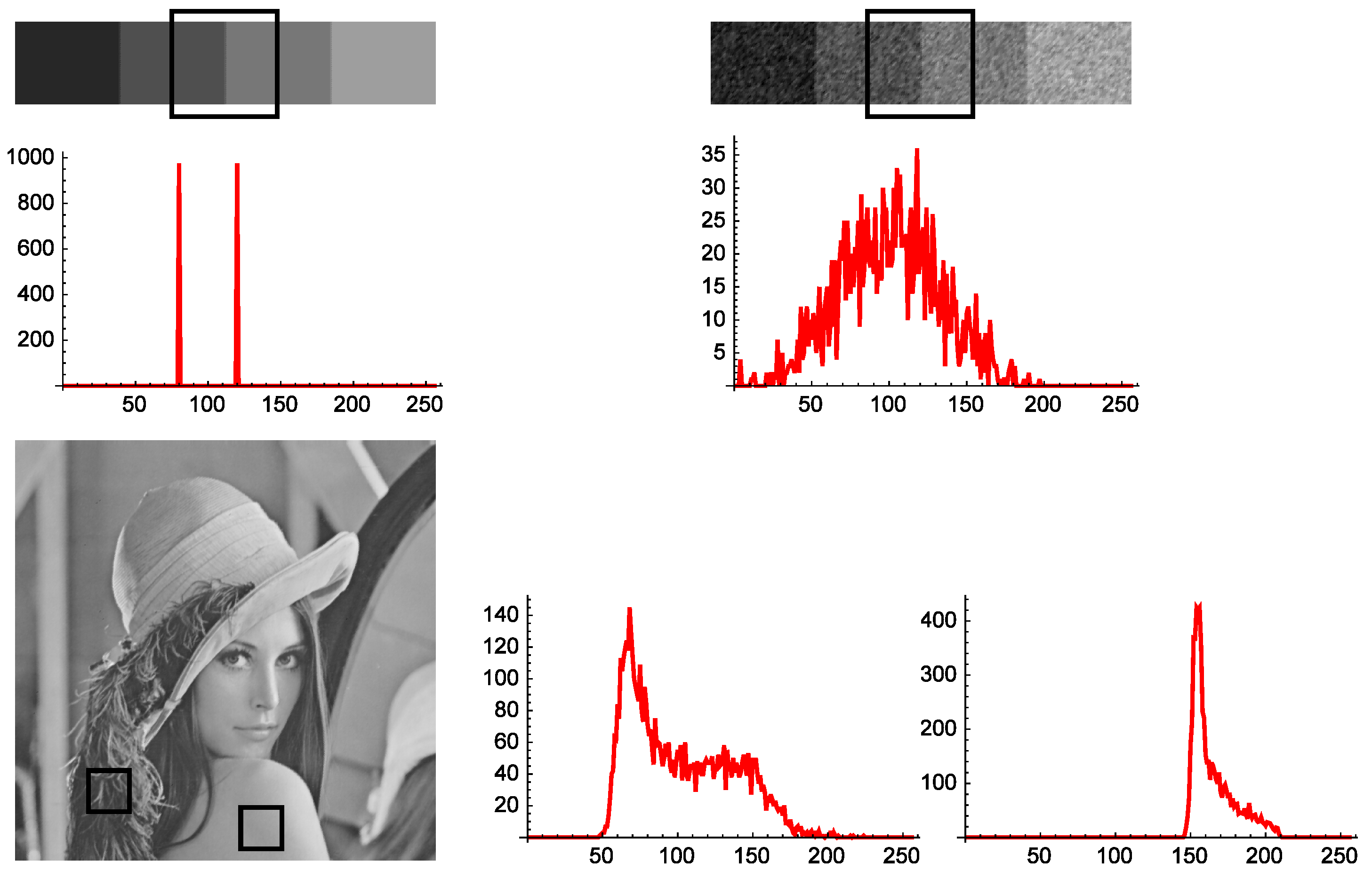
As has been explained in Section 2, Jensen–Shannon divergence is a measure of dissimilarity or inverse cohesion between two (or more) probability distributions. In the case of two probability distributions, if those are representative of two different regions in an image, then this fact can be used to guess whether they are coming from the same object or not. A way to get representative information of the composition of a given object or texture inside an image is by means of the histogram, as the distribution of gray levels (or colors) of a sample. The histogram (see Figure 1) tells us about the gray level variety and composition, not about the location of pixels.

Figure 1 show three images, and the histograms of some image samples are presented. In the histograms, the horizontal axis in the graph is the gray level, and the vertical axis is the corresponding absolute frequency. As can be seen, in the first image, the region marked by the square is entirely composed of only two gray levels. Thus, the corresponding histogram, below the image, contains only two nonzero frequencies. The second example is the previous image corrupted by a Gaussian noise of mean zero and sigma 20. Obviously, the noise produces in the histogram, below the image, a great dispersion of gray levels, with a loss of information. The third image is Lenna. This image has a lot of very different regions. Feathers in her hat (first histogram at the right) show a characteristic gray level distribution with a wide range of colors. However, the shoulder of Lenna (second histogram at the right) has a histogram with less scattering of gray levels.

Figure 1. Histograms of square samples from several images. In the first case (top left), there are only two gray levels with the same absolute frequency. The second case (top right) corresponds to the previous image affected by gaussian noise, so that a strong scattering of the histogram can be appreciated. In the image of Lenna, the first histogram (left) corresponds to shoulders and the right histogram to feathers.

Figure 1. Histograms of square samples from several images. In the first case (top left), there are only two gray levels with the same absolute frequency. The second case (top right) corresponds to the previous image affected by gaussian noise, so that a strong scattering of the histogram can be appreciated. In the image of Lenna, the first histogram (left) corresponds to shoulders and the right histogram to feathers.

In general, we expect that histograms coming from different parts of the same object will be similar, but histograms coming from diverse objects will be different. This is the principle we will use to detect edges. In order to apply $JS$ as an edge detector, two neighbor samples S₁ and S₂ are taken along the whole image by means of a double sliding window centered on every pixel of the image. Unweighted Jensen–Shannon divergence of the corresponding normalized histograms $P_1$ and $P_2$ tells us about the similarity of the samples and, likely, will allow us to decide if the two samples are coming from the same object, the same region or are not in the image. In this way, if divergence between $S_1$ and $S_2$ is low, it means that both samples are very similar, probably coming from the same region. Conversely, if divergence is high, then $S_1$ and $S_2$ are quite different, almost certainly coming from two different regions.

Several orientations of the double window should be taken for each pixel image. This is to properly detect edges in any direction and to avoid a bias towards edges in a particular course. Due to the special discrete nature of digital images, four basic orientations are the simplest to use: 0, 45, 90 and 135 degrees (that we transform into 0, $\frac{1}{4}$, $\frac{1}{2}$ and $\frac{3}{4}$ linearly). Thus, associated with each pixel, four divergences $d_1$, $d_2$, $d_3$ and $d_4$ are obtained in practice. The best way to combine them into a unique measure is by interpolating a periodic function, such as [6]:

$$JS\left(d\right)\approx c+msin\left(2\pi d\right)+ncos\left(2\pi d\right),d\in [0,1]$$

(4)

where c, m and n are constants to be adjusted. Since the cost of the numerical computation of trigonometric functions is high, we prefer to approximate such functions by quadratic splines, which are second degree piecewise polynomials having class 1 (with a continuous derivative). Therefore, we obtain,

$$sin\left(2\pi x\right)\approx \psi \left(x\right)=\left\{\begin{array}{cc}-16x^2+8x,\hfill & \mathrm{if}x\in [0,\frac{1}{2}]\hfill \\ 16x^2-24x+8,\hfill & \mathrm{if}x\in [\frac{1}{2},1].\hfill \end{array}\right.$$

(5)

and the cosine function in $JS$ can be similarly approximated by:

$$cos\left(2\pi x\right)\approx \varphi \left(x\right)=\left\{\begin{array}{cc}-16x^2+1,\hfill & \mathrm{if}x\in [0,\frac{1}{4}]\hfill \\ 16x^2-16x+3,\hfill & \mathrm{if}x\in [\frac{1}{4},\frac{3}{4}]\hfill \\ -16x^2+32x-15,\hfill & \mathrm{if}x\in [\frac{3}{4},1].\hfill \end{array}\right.$$

(6)

These functions are periodic spline functions of degree two and class 1, defined in $[0,1]$ with nodes at the points $\{0,\frac{1}{4},\frac{1}{2},\frac{3}{4},1\}$. Using the result in [6], we can approximate $JS\left(d\right)$ as a function of the direction in terms of the spline approximate for the trigonometric functions $\left\{\psi \right(x),\varphi (x\left)\right\}$; together with the least-square fit, we can write $JS\left(d\right)$ as,

$$JS\left(d\right)=\frac{d_1+d_2+d_3+d_4}{4}+\frac{d_2-d_4}{2}\psi \left(d\right)+\frac{d_1-d_3}{2}\varphi \left(d\right).$$

(7)

Simple analysis for the values of $d_i,i=1,2,3,4$ could provide us with the direction of maximum divergence, as shown in the following list, and finally, the divergence associated with the pixel at hand is the maximum value of the spline function, $JS\left(d\right)$, except singularities (for example in a homogeneous region, in which case the direction has no sense).

If	then the maximum attains at
$d_1-d_3\ge 0$, $d_2-d_4\ge 0$	$d=\frac{d_2-d_4}{4(d_1-d_3)-(d_2-d_4)}$	$\in {[0,\frac{1}{4}]}_{}^{}$
$d_1-d_3\ge 0$, $d_2-d_4\le 0$	$d=\frac{4(d_1-d_3)-3(d_2-d_4)}{4(d_1-d_3)-(d_2-d_4)}$	$\in [\frac{3}{4},1]$
$d_1-d_3\le 0$, $d_2-d_4\ge 0$	$d=\frac{2(d_1-d_3)-(d_2-d_4)}{4(d_1-d_3)-(d_2-d_4)}$	$\in [\frac{1}{4},\frac{1}{2}]$
$d_1-d_3\le 0$, $d_2-d_4\le 0$	$d=\frac{2(d_1-d_3)+3(d_2-d_4)}{4(d_1-d_3)-(d_2-d_4)}$	$\in [\frac{1}{2},\frac{3}{4}]$

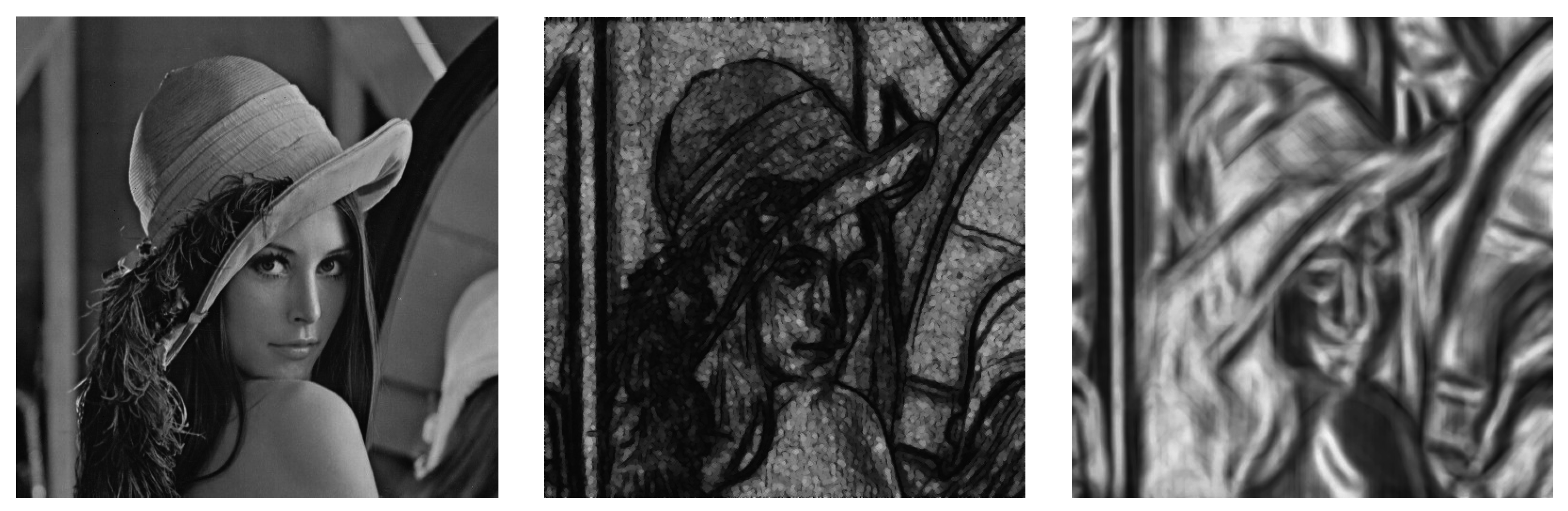
By means of this procedure, two real numbers, divergence and direction, are associated with each pixel in the image. In the sequel we consider only the first one. If it is low, then the pixel is likely interior to a region, and if it is high, then the pixel is likely an edge. Now, we can represent this matrix of divergences in a visual fashion. The example shown in Figure 2 on the right represents a divergence matrix. Light pixels correspond to low divergences, hence to the interior of regions, while dark pixels are rather frontiers between regions. The original image is of Lenna.

Figure 2. Left: Picture of Lenna, a real scene. Middle: smoothed $JS$ matrix of Lenna processed with semicircular sliding windows of radius 3. Right: the same as the previous image, but using semicircular sliding windows of radius 20. Smoothing procedure is explained below in this Section.

Figure 2. Left: Picture of Lenna, a real scene. Middle: smoothed $JS$ matrix of Lenna processed with semicircular sliding windows of radius 3. Right: the same as the previous image, but using semicircular sliding windows of radius 20. Smoothing procedure is explained below in this Section.

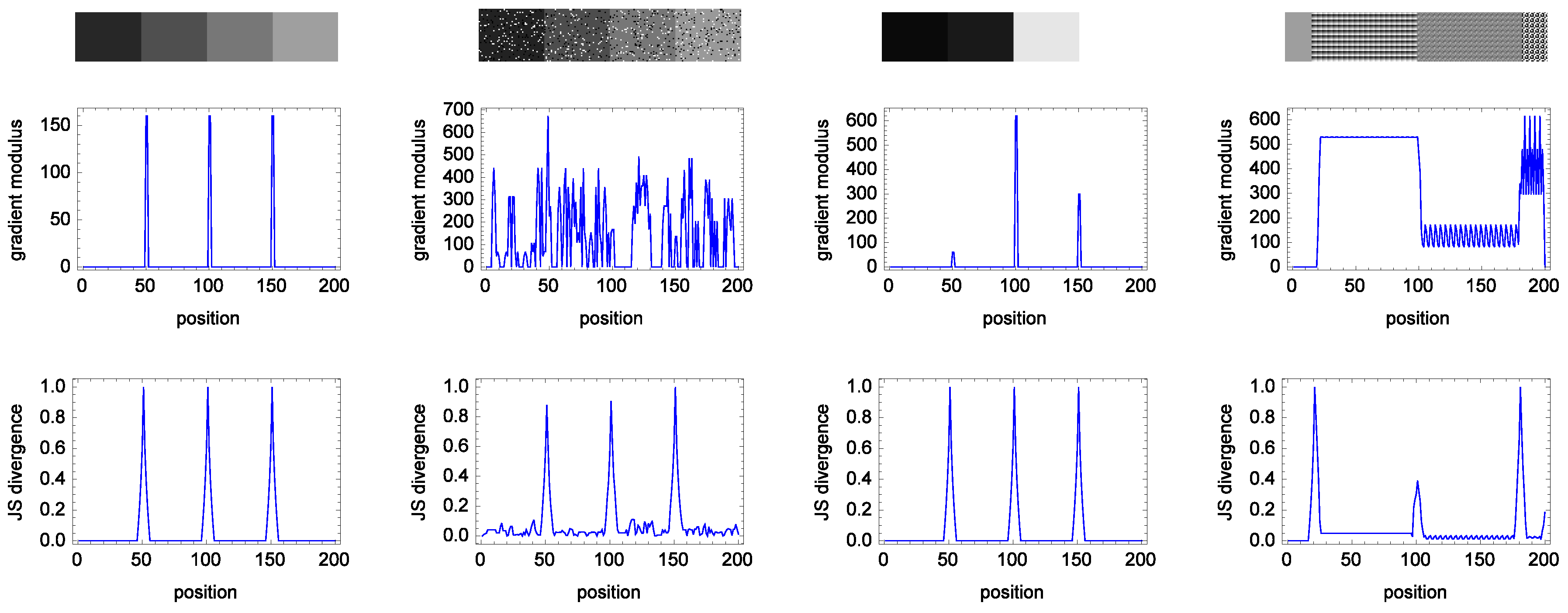
Figure 3 shows four test images. The first image is made of four different solid gray levels. In the second row, three sharp leaps can be seen in a line of the modulus of the gradient obtained applying the Sobel edge detector to Image 1. The leaps match the transitions from one homogeneous region to the next. Under this graph, there is another one corresponding to a line of edge detection obtained applying $JS$ to Image 1, with two square semi-windows with a size of $5\times 5$ (this size is used in all of the images in Figure 3). Both edge methods detect all of the edges present in Image 1. Due to that the image being clean, free of noise and textures, and the boundary between the regions being straight, the edge detection is easy.

Figure 3. Four test images (top row) for edge detection. Image 1: a synthetic image made of four homogeneous regions with different, equally-spaced gray levels. Image 2: the same image as the first corrupted by salt and pepper noise over $10\%$ of the image pixels. Image 3: an image composed of four different gray levels, with different distances between gray levels. Image 4: an image composed of four different textures. Second row: representation, along a horizontal line in the middle of each image, of the respective gradient modules of the images, using the Sobel mask. Third row: corresponding representation of the $JS$ of the images using two square semi-windows with a $5\times 5$ size.

Figure 3. Four test images (top row) for edge detection. Image 1: a synthetic image made of four homogeneous regions with different, equally-spaced gray levels. Image 2: the same image as the first corrupted by salt and pepper noise over $10\%$ of the image pixels. Image 3: an image composed of four different gray levels, with different distances between gray levels. Image 4: an image composed of four different textures. Second row: representation, along a horizontal line in the middle of each image, of the respective gradient modules of the images, using the Sobel mask. Third row: corresponding representation of the $JS$ of the images using two square semi-windows with a $5\times 5$ size.

The second image is the same as the previous image, but corrupted by impulsive salt-and-pepper noise affecting $10\%$ of the image pixels. As can be seen, the gradient plot looks random. Nevertheless, edge detection using $JS$ allows one to get all edges.

The third image is made of four different homogenous gray level bands, but the distance between gray levels is different in the three frontiers present in the image. In the corresponding plot of gradients for this image, the left frontier has a very much lower gradient than the others, being the highest the central one. However, in the corresponding $JS$ plot, both borders have been detected with the same $JS$ value.

Finally, the fourth image presents four different textures. The detection with Sobel is impossible, as can be seen in the corresponding gradient plot. Nevertheless, $JS$ detects all of the borders correctly.

If the $JS$ value is low for a given pixel, then the pixel is likely interior to a region. Conversely, if the $JS$ value is high, then the pixel is likely an edge. However, in practice, due to the presence of textures, noise or any other statistical fluctuations, the image may contain many small irregularities that could lead the $JS$ calculation to many local maxima with very low value. Then, it is advisable to apply a smoothing median-like filter to the calculated divergences. Since it is important not to lose directional local maximum divergences, a common median filter $3\times 3$ is not advisable. We are interested in preserving directional local maxima. Hence, the following smoothing algorithm may be iteratively applied until the root is reached:

-

Center a $3\times 3$ window on each position of the divergence matrix and get a sample of nine JSs.

-

Consider all sets of three pixels aligned in the four main directions containing the central pixel. Take the four corresponding median values.

-

Output the maximum of both the central divergence and the four medians.

In this paper all divergences matrices are smoothed by means of this procedure.

Note that by using $JS$, we are detecting not only gradients, as many methods do, but also many structural and texture differences between samples (see Image 4 in Figure 3).

Figure 2 illustrates a common problem in the edge detection field: a window size that is too small leads to an over-segmented image, with many undesired pixels marked as edges. Additionally, a window size that is too big leads to blurred and misplaced edge detection. Since the adequate window size depends on the objects present in the image, in general, then, the correct election of the window size should be done by the user. In the next section, a multi-size window strategy is described to deal with this problem.

4. The Size of the Sliding Window

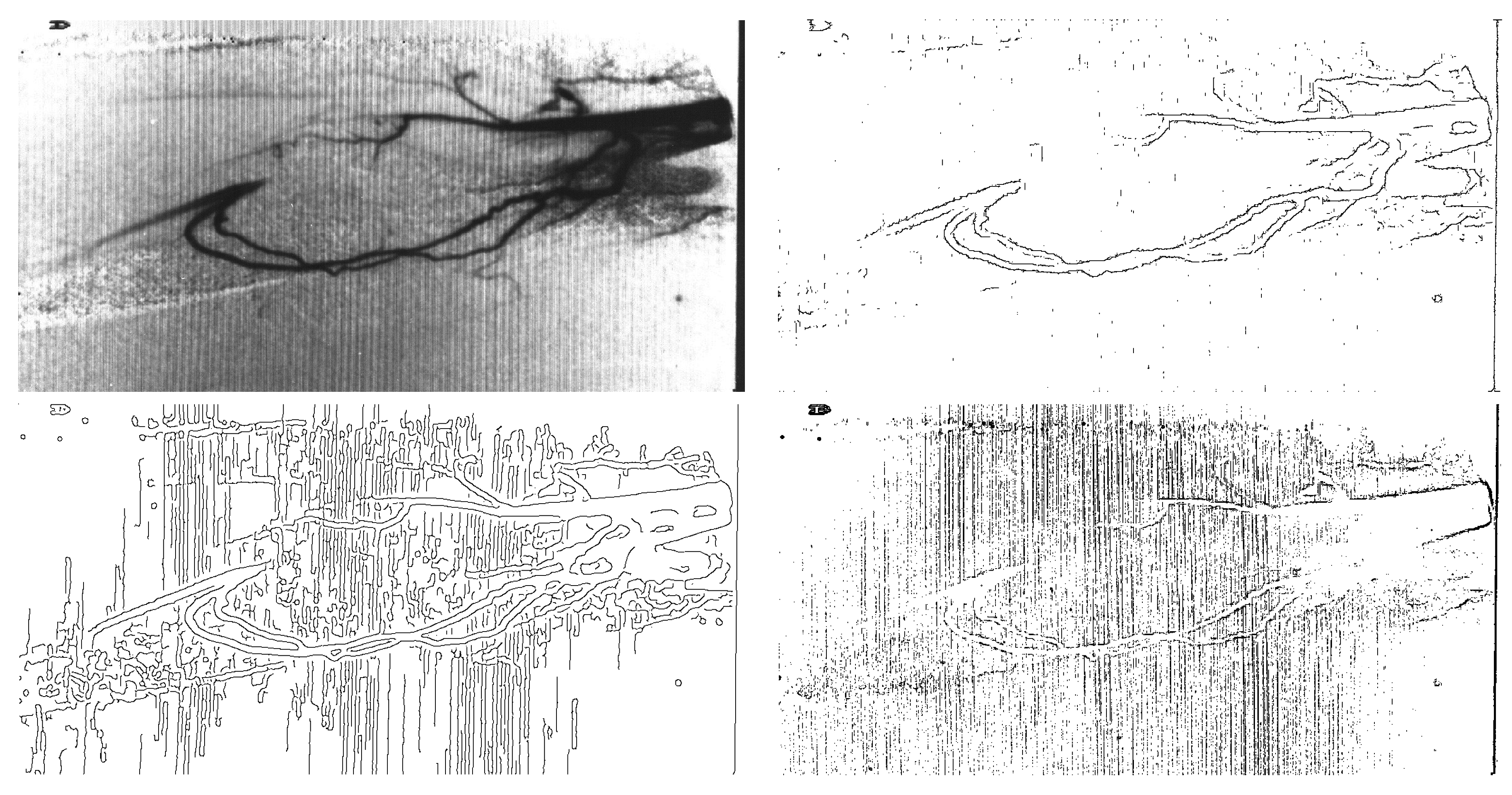
The use of a double sliding window clearly implies that some choices must be done by the user, namely the shape and the size. With respect to the shape, we have decided to use at all times a round window divided into two semicircles. This is the most unbiased decision with respect to all directions. Obviously, all this has to be adapted to the discrete array of pixels in a digital image. However, the size cannot be setup independently of the image. This is a factor bound to the particular image at hand, the size of the objects and the resolution. 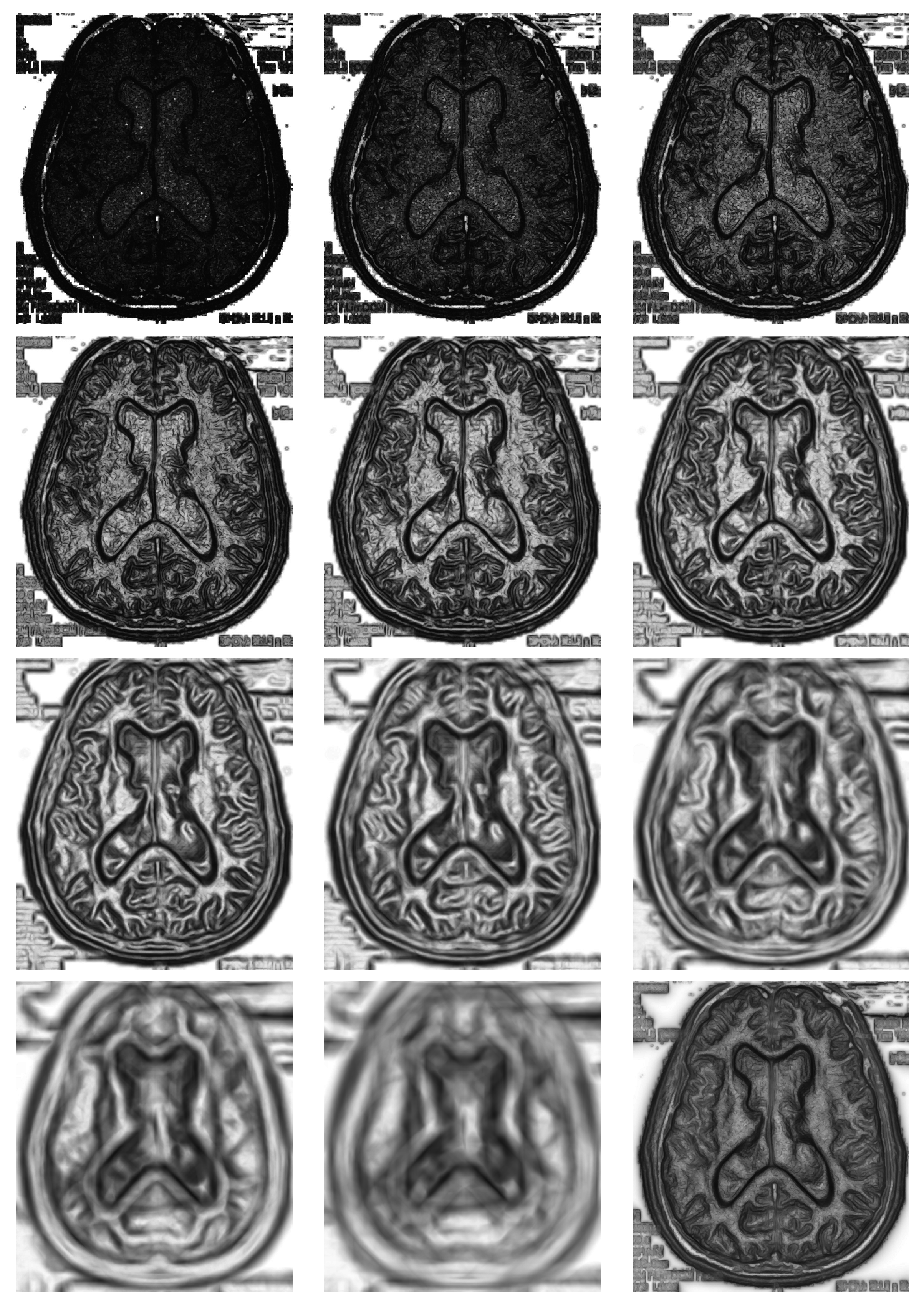In Figure 4, we show the matrix of divergences for several radii $\{2,3,4,6,8,11,16,23,32,45,64\}$ distributed as a rounded geometric progression of a ratio of $\sqrt{2}$; the corresponding images show good and bad choices of the radius. The choice of a size that is too small can give something like the first image on the top at the left, where many divergences are very high, thus saturated, and objects will be hardly detected, because they are hidden among many unimportant details. Conversely, a size that is too big, apart from the high computation time, can lead us to something like the image at the right at the bottom, cleaner, but where edges appear very blurred and a little out of place.

It may be that choosing a particular radius could be adequate for a particular image. If we do not know what is the range of sizes of the objects to be detected in the image at hand, then it is advisable to use several window sizes at the same time and, finally, combining them in a convenient way. To do this, we chose a set of different radii and take for each image pixel the mean of the divergences, as is shown in the last figure on the bottom in Figure 4.

In right bottom image of Figure 4 is shown the average divergence matrix corresponding to eleven different radii from two to 64 in a geometric progression. Depending on what we need, this last could be more adequate than a particular radius to obtain a good segmentation, as described in the next section. In addition, this choice makes the general procedure more independent of the double window size, since the problem of adjusting the radius is automated. 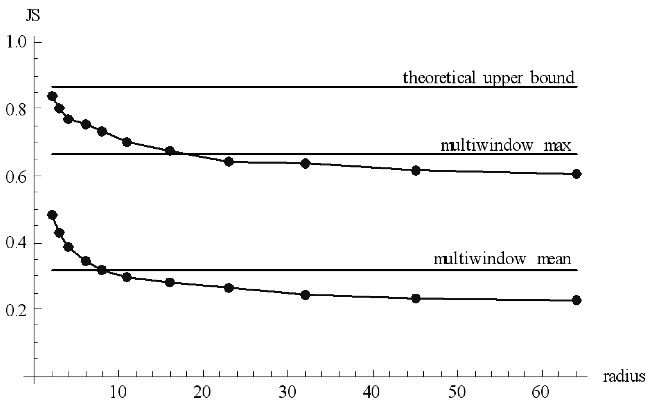Figure 5 shows the variation of maximum and mean divergence in the matrix for the experiment of Figure 4 (Brain), depending on the radius.

Figure 4. In this figure, we compute divergence matrices for radii of $\{2,3,4,6,8,11,16,23,32,45,64\}$, respectively from top to down, left to right. In the last picture, we used multi-size window.

Figure 4. In this figure, we compute divergence matrices for radii of $\{2,3,4,6,8,11,16,23,32,45,64\}$, respectively from top to down, left to right. In the last picture, we used multi-size window.

Figure 5. Variation of the maximum and mean divergence in the matrix for the experiment of Figure 4 (Brain), depending on the radius.

Figure 5. Variation of the maximum and mean divergence in the matrix for the experiment of Figure 4 (Brain), depending on the radius.

5. Edge Detection: Binarization

In this section, we will explain the binarization of the divergence matrix, a way to select the final edge pixels. Starting from the divergences matrix, the simplest binarization method is by thresholding. Pixels having a $JS$ value lower than the threshold are considered interior to a region, thus marked as not belonging to an edge, and pixels having $JS$ higher than the threshold are in edges. In general, this procedure is primitive and does not give satisfactory results, since we can get thick edges while loosing other edges. Another idea is to search for some kind of local maxima in the matrix. Since we are working in two dimensions, local maxima will be searched in those four principal directions. A pixel is considered as belonging to an edge if the $JS$ is a local maximum in at least one of the four principal directions. To do this, a set of four unidimensional windows in the principal directions is placed over each image pixel. Then, a pixel is declared as an edge if, at least in one direction, it fulfills the following:

• The central $JS$ is not less than all of the other $JS$ values in the window
• There is at least one pixel within the window with a $JS$ value lower than the central one in a threshold set by the user.

In Section 6, an example of this edge selection procedure is presented, together with a comparison of our multi-radius sliding window procedure with the Canny and Sobel edge detectors.

Figure 6. In this figure we see on the top row an original image of an angiogram with its edges detected by using the multi-window procedure with the same set of radii as in Figure 4; on the second row, we see the results obtained using the Canny method (left) and the Sobel method (right); both methods fail at detecting the edges due to noise and vertical textures.

Figure 6. In this figure we see on the top row an original image of an angiogram with its edges detected by using the multi-window procedure with the same set of radii as in Figure 4; on the second row, we see the results obtained using the Canny method (left) and the Sobel method (right); both methods fail at detecting the edges due to noise and vertical textures.

6. Applications and Comparisons with Other Edge Detectors

In this section, we compare our method of edge detection with two well-known edge detection methods, Canny [18] and Sobel [19] filters. In Figure 6, an angiogram picture (top left) and the final edge images obtained with $JS$ (top right), Canny (bottom left) and Sobel (bottom right) are shown. It is clear that the best image of edges is that obtained with the proposed multi-window method, which his very superior to the results of the Canny and Sobel edge detectors. One of the applications of the segmentation of this picture is the measurement of the width of the veins and arteries and to automatically detect stenosis.

7. Conclusions

In this paper, a new entropic edge detection method based on the Jensen–Shannon divergence is presented. The method works by calculating the Jensen–Shannon divergence between the normalized histograms of two adjacent semicircular sliding windows. The election of a particular size of window is avoided by performing a multi-window computation and then computing for each image pixel the mean Jensen–Shannon divergence of each window size.

One of the main advantages of using Jensen–Shannon divergence is the property of being invariant to contrast and robust against noise in the picture. This gives the method a big advantage over other usual edge detection methods. Some experiments performed using medical images show that our method is very superior compared to the Canny and Sobel edge detectors.