Article

A Clustering Method Based on the Maximum Entropy Principle

1
Instituto de Investigaciones en Matemáticas Aplicadas y en Sistemas, Universidad Nacional Autónoma de México, Ciudad Universitaria, 04510 Ciudad de México, Mexico
2
Instituto Tecnológico Autónomo de México, Río Hondo 1. Col. Progreso Tizapán, 01080 Ciudad de México, Mexico
*
Author to whom correspondence should be addressed.
Entropy 2015, 17(1), 151-180; https://doi.org/10.3390/e17010151
Submission received: 6 October 2014 / Accepted: 26 December 2014 / Published: 7 January 2015
(This article belongs to the Section Information Theory, Probability and Statistics)

Abstract

:
Clustering is an unsupervised process to determine which unlabeled objects in a set share interesting properties. The objects are grouped into k subsets (clusters) whose elements optimize a proximity measure. Methods based on information theory have proven to be feasible alternatives. They are based on the assumption that a cluster is one subset with the minimal possible degree of “disorder”. They attempt to minimize the entropy of each cluster. We propose a clustering method based on the maximum entropy principle. Such a method explores the space of all possible probability distributions of the data to find one that maximizes the entropy subject to extra conditions based on prior information about the clusters. The prior information is based on the assumption that the elements of a cluster are “similar” to each other in accordance with some statistical measure. As a consequence of such a principle, those distributions of high entropy that satisfy the conditions are favored over others. Searching the space to find the optimal distribution of object in the clusters represents a hard combinatorial problem, which disallows the use of traditional optimization techniques. Genetic algorithms are a good alternative to solve this problem. We benchmark our method relative to the best theoretical performance, which is given by the Bayes classifier when data are normally distributed, and a multilayer perceptron network, which offers the best practical performance when data are not normal. In general, a supervised classification method will outperform a non-supervised one, since, in the first case, the elements of the classes are known a priori. In what follows, we show that our method’s effectiveness is comparable to a supervised one. This clearly exhibits the superiority of our method.

1. Introduction

Pattern recognition is a scientific discipline whose methods allow us to describe and classify objects. The descriptive process involves the symbolic representation of these objects through a numerical vector x :
x = [ x 1 , x 2 , x n ] n
where its n components represent the value of the attributes of such objects. Given a set of objects (“dataset”) X, there are two approaches to attempt the classification: (1) supervised; and (2) unsupervised.
In the unsupervised approach case, no prior class information is used. Such an approach aims at finding a hypothesis about the structure of X based only on the similarity relationships among its elements. These relationships allow us to divide the space of X into k subsets, called clusters. A cluster is a collection of elements of X, which are “similar” between them and “dissimilar” to the elements belonging to other clusters. Usually, the similarity is defined by a metric or distance function d: X × X → ℜ [13]. The process to find the appropriate clusters is typically denoted as a clustering method.

1.1. Clustering Methods

In the literature, many clustering methods have been proposed [4,5]. Most of them begin by defining a set of k centroids (one for each cluster) and associating each element in X with the nearest centroid based on a distance d. This process is repeated, until the difference between centroids at iteration t and iteration t − 1 tends to zero or when some other optimality criterion is satisfied. Examples of this approach are k-means [6] and fuzzy c-means [79]. Other methods not following the previous approach are: (1) hierarchical clustering methods that produce a tree or a graph in which, during the clustering process, based on some similarity measure, the nodes (which represent a possible cluster) are merged or split; in addition to the distance measure, we must also have a stopping criterion to tell us whether the distance measure is sufficient to split a node or to merge two existing nodes [1012]; (2) density clustering methods, which consider clusters as dense regions of objects in the dataset that are separated by regions of low density; they assume an implicit, optimal number of clusters and make no restrictions with respect to the form or size of the distribution [13]; and (3) meta-heuristic clustering methods that handle the clustering problem as a general optimization problem; these imply a greater flexibility of optimization algorithms, but also longer execution times [14,15].
We propose a numerical clustering method that lies in the group of meta-heuristic clustering methods, where the optimization criterion is based on information theory. Some methods with similar approaches have been proposed in the literature (see Section 1.6).

1.2. Determining the Optimal Value of k

In most clustering methods, the number k of clusters must be explicitly specified. Choosing an appropriate value has important effects on the clustering results. An adequate selection of k should consider the shape and density of the clusters desired. Although there is not a generally accepted approach to this problem, many methods attempting to solve it have been proposed [5,16,17]. In some clustering methods (such as hierarchical and density clustering), there is no need to explicitly specify k. Implicitly, its value is, nevertheless, still required: the cardinality or density of the clusters must be given. Hence, there is always the need to select a value of k. In what follows, we assume that the value of k is given a priori. We do not consider the problem of finding the optimal value of k. See, for example, [1820].

1.3. Evaluating the Clustering Process

Given a dataset X to be clustered and a value of k, the most natural way to find the clusters is to determine the similarity among the elements of X. As mentioned, usually, such similarity is established in terms of proximity through a metric or distance function. In the literature, there are many metrics [
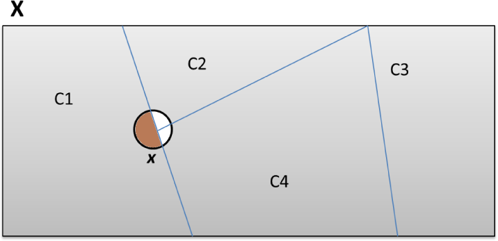
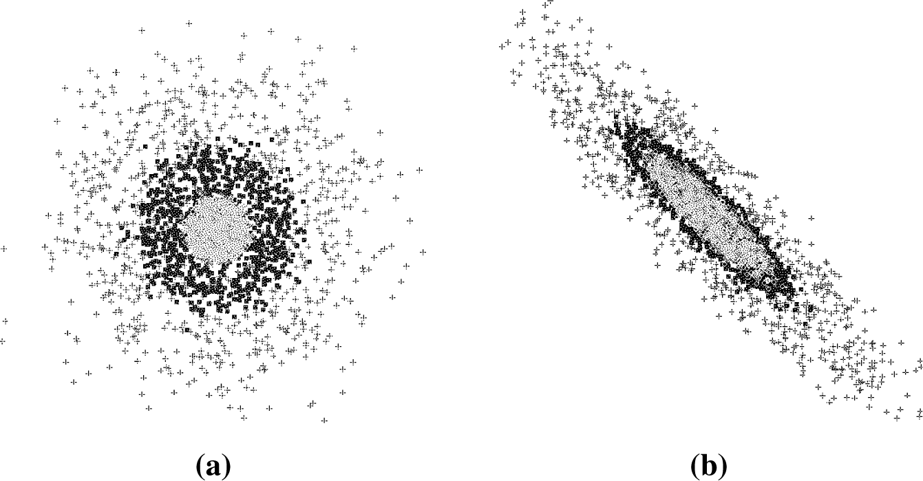
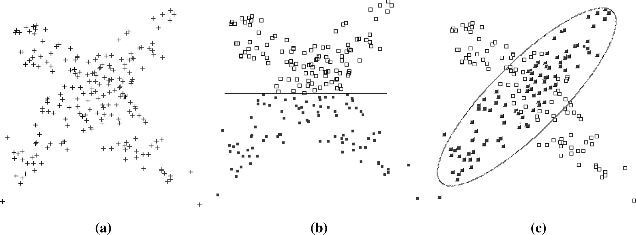
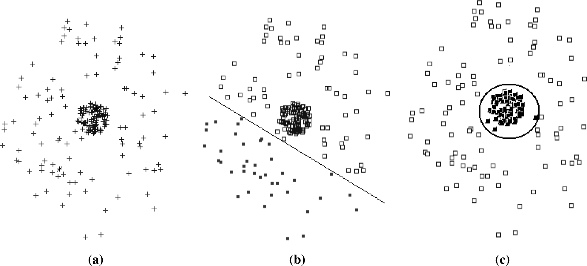
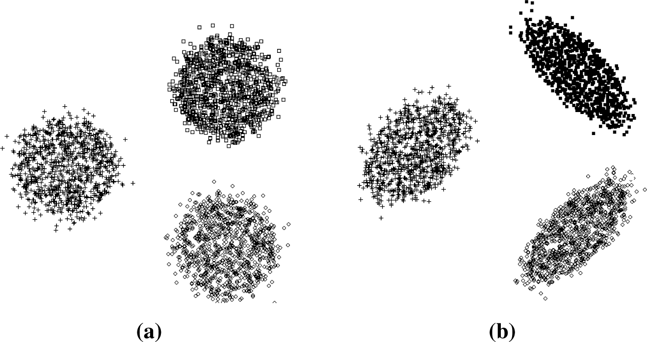
21] that allow us to find a variety of clustering solutions. The problem is how to determine if a certain solution is good or not. For instance, in Figures 1 and 2, we can see two datasets clustered with k = 2. For such datasets, there are several possible solutions, as shown in Figures 1b,c and 2b,c, respectively.
Frequently, the goodness of a clustering solution is quantified through validity indices [4,8,22,23]. The indices in the literature are classified into three categories: (1) external indices that are used to measure the extent to which cluster labels match externally-supplied class labels (F-measure [24], NMIMeasure [25], entropy [26], purity [27]); (2) internal indices, which are used to measure the goodness of a clustering structure with respect to the intrinsic information of the dataset ([8,2831]); and (3) relative indices that are used to compare two different clustering solutions or particular clusters (the RAND index [32] and adjusted RAND index [33]).
Clusters are found and then assigned a validity index. We bypass the problem of qualifying the clusters and, rather, define a quality measure and then find the clusters that optimize it. This allows us to define the clustering process as follows:
Definition 1. Given a dataset X to be clustered and a value of k, clustering is a process that allows the partition of the space of X into k regions, such that the elements that belong to them optimize a validity index q.
Let Ci be a partition of X and Π = {C1, C2, …Ck} the set of such partitions that represents a possible clustering solution of X. We can define a validity index q as a function of the partition set Π, such that the clustering problem may be reduced to an optimization problem of the form:
Optimize q = f ( Π ) subject to : g i ( Π ) 0 , i = 1 , 2 , m h j ( Π ) = 0 , j = 1 , 2 , , p
where gi and hj are constraints, likely based on prior information about the partition set Π (e.g., the desired properties of the clusters).
We want to explore the space of those feasible partition sets and find one that optimizes a validity index instead, doing an a posteriori evaluation of a partition set (obtained by any optimization criterion) through such an index. This approach allows us to find “the best clustering” within the limits of a validity index. To tightly confirm such an assertion, we resort to the statistical evaluation of our method (see Section 5).

1.4. Finding the Best Partition of X

Finding the suitable partition set Π of X is a difficult problem. The total number of different partition sets of the form Π = {C1, C2, …Ck} may be expressed by the function S(N, k) associated with the Stirling number of the second kind [34], which is given by:
S ( N , k ) = 1 k ! i = 0 k ( 1 ) k i ( i k ) i N
where N = |X|. For instance, for N = 50 and k = 2, S(N, k) ≈ 5.63 × 10¹⁴. This number illustrates the complexity of the problem that we need to solve. Therefore, it is necessary to resort to a method that allows us to explore efficiently a large solution space. In the following section, we briefly describe some meta-heuristic searches.

1.5. Choosing the Meta-Heuristic

During the last few decades, there has been a tendency to consider computationally-intensive methods that can search very large spaces of candidate solutions. Among the many methods that have arisen, we mention tabu search [3537], simulated annealing [38,39], ant colony optimization [40], particle swarm optimization [41] and evolutionary computation [42]. Furthermore, among the many variations of evolutionary computation, we find evolutionary strategies [43], evolutionary programming [44], genetic programming [45] and genetic algorithms (GAs) [46]. All of these methods are used to find approximate solutions for complex optimization problems. It was proven that an elitist GA always converges to the global optimum [47]. Such a convergence, however, is not bounded in time, and the selection of the GA variation with the best dynamic behavior is very convenient. In this regard, we rely on the conclusions of previous analyses [48,49], which showed that a breed of GA, called the eclectic genetic algorithm (EGA), achieves the best relative performance. Such an algorithm incorporates the following:
  • Full elitism over a set of size n of the last population. Given that, by generation t, the number of individual tested is nt, the population in such a generation consists of the best n individuals.
  • Deterministic selection as opposed to the traditional proportional selection operator. Such a scheme emphasizes genetic variety by imposing a strategy that enforces the crossover of predefined individuals. After sorting the individual’s fitness from better to worse, the i-th individual is combined with the (ni + 1)-th individual.
  • Annular (two-point) crossover.
  • Random mutation of a percentage of bits of the population.
In Appendix A, we present the pseudocode of EGA. The reader can find detailed information in [4851].

1.6. Related Works

Our method is meta-heuristic (see Section 1.1). The main idea behind our method is to handle the clustering problem as a general optimization problem. There are various suitable meta-heuristic clustering methods. For instance, in [5254], three different clustering methods based on differential evolution, ant colony and multi-objective programming, respectively, are proposed.
Both meta-heuristic or analytical methods (iterative, density-based, hierarchical) have objective functions, which are associated with a metric. In our method, the validity index becomes the objective function.
Our objective function is based on information theory. Several methods based on the optimization of information theoretical functions have been studied [5560]. Typically, they optimize quantities, such as entropy [26] and mutual information [61]. These quantities involve determining the probability distribution of the dataset in a non-parametric approach, which does not make assumptions about a particular probability distribution. The term non-parametric does not imply that such methods completely lack parameters; they aim to keep the number of assumptions as weak as possible (see [57,60]). Non-parametric approaches involve density functions, conditional density functions, regression functions or quantile functions in order to find the suitable distribution. Typically, such functions imply tuning parameters that determine the convergence of searching for the optimal distribution.
A common clustering method based on information theory is ENCLUS (entropy clustering) [62], which allows us to split iteratively the space of the dataset X in order to find those subspaces that minimize the entropy. The method is motivated by the fact that a subspace with clusters typically has lower entropy than a subspace without clusters. In order to split the space of X, the value of a resolution parameter must be defined. If such a value is too large, the method may not able to capture the differences in entropy in different regions in the space.
Our proposal differs from traditional clustering methods (those based on minimizing a proximity measure as k-means or fuzzy c-means) in that, instead of finding those clusters that optimize such a measure and then defining a validity index to evaluate its quality, our method finds the clusters that optimize a purported validity index.
As mentioned, such a validity index is an information theoretical function. In this sense, our method is similar to those mentioned methods based on information theory. However, it does not use explicitly a non-parametric approach to find the distribution of the dataset. It explores the space of all possible probability distributions to find one that optimizes our validity index. For this reason, the use of a suitable meta-heuristic is compulsory. With the exception of the parameters of such a meta-heuristic, our method does not resort to additional parameters to find the optimal distribution and, consequently, the optimal clustering solution.
Our validity index involves entropy. Usually in the methods based on information theory, the entropy is interpreted as a “disorder” measure; thus, an obvious way is to minimize such a measure. In our work, we propose to maximize it due to the maximum entropy principle.

1.7. Organization of the Paper

The rest of this work is organized as follows: In Section 2, we briefly discuss the concept of information content, entropy and the maximum entropy principle. Then, we approach such issues in the context of the clustering problem. In Section 3, we formalize the underlying ideas and describe the main line of our method (in what follows, clustering based on entropy (CBE)). In Section 4, we present a general description of the datasets. Such datasets were grouped into three categories: (1) synthetic Gaussian datasets; (2) synthetic non-Gaussian datasets; and (3) experimental datasets taken from the UCIdatabase repository. In Section 5, we present the methodology to evaluate the effectiveness of CBE regardless of a validity index. In Section 6, we show the experimental results. We use synthetically-generated Gaussian datasets and apply a Bayes classifier (BC) [6365]. We use the results as a standard for comparison due to its optimal behavior. Next, we consider synthetic non-Gaussian datasets. We prove that CBE yields results comparable to those obtained by a multilayer perceptron network (MLP). We show that our (non-supervised) method’s results are comparable to those of BC and MLP, even though these are supervised. The results of other clustering methods are also presented, including an information theoretic-based method (ENCLUS). Finally, in Section 7, we present our conclusions. We have included three appendices expounding important details.

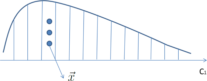
2. Maximum Entropy Principle and Clustering

The so-called entropy [26] appeals to an evaluation of the information content of a random variable Y with possible values {y1, y2, …yn}. From a statistical viewpoint, the information of the event (Y = yi) is inversely proportional to its likelihood. This information is denoted by I(yi), which can be expressed as:
I ( y i ) = log ( 1 p ( y i ) ) = log ( p ( y i ) )
From information theory [26,66], the entropy of Y is the expected value of I. It is given by:
H ( Y ) = i = 1 N p ( y i ) log ( p ( y i ) )
Typically, the log function may be taken to be log2, and then, the entropy is expressed in bits; otherwise, as ln, in which case the entropy is in nats. We will use log2 for the computations in this paper.
When p(yi) is uniformly distributed, the entropy of Y is maximal. This means that Y has the highest level of unpredictability and, thus, the maximal information content. Since entropy reflects the amount of “disorder” of a system, many methods employ some form of such a measure in the objective function of clustering. It is expected that each cluster has a low entropy, because data points in the same cluster should look similar [5660].
We consider a stochastic system with a set of states S = {Π1, Π2, …, Πn} whose probabilities are unknown (recall that Πi is a likely partition set of X of the form Π = {C1, C2, …, Ck}). A possible assertion would be that the probabilities of all states are equal (p1) = p2) = … = pn−1) = pn)), and therefore, the system has the maximum entropy. However, if we have additional knowledge, then we should be able to find a probability distribution that is better in the sense that it is less uncertain. This knowledge can consist of certain average values or bounds on the probability distribution of the states, which somehow define several conditions imposed upon such distribution. Usually, there is an infinite number of probability models that satisfies these conditions.
The question is: which model should we choose? The answer lies in the maximum entropy principle, which may be stated as follows [67]: when an inference is made on the basis of incomplete information, it should be drawn from the probability distribution that maximizes the entropy, subject to the constraints on the distribution. As mentioned, a condition is an expected value of some measure about the probability distributions. Such a measure is one for which each of the states of the system has a value denoted by gi).
For example, let X = {9, 10, 9, 2, 1} be a discrete dataset to be clustered with k = 2. We assume that the “optimal” labeling of the dataset is the one that is shown in Table 1.
Such labeling defines a partition Π* of the form Π* = {C1 = {9, 10, 9}, C2 = {2, 1}}. The probability model of Π* is given by the conditional probabilities p(x|Ci) that represent the likelihood that, when observing cluster Ci, we can find object x. Table 2 shows such probabilities.
The entropy of X conditioned on the random variable C taking a certain value Ci is denoted as H(X|C = Ci). Thus, we define the total entropy of Π* as:
H ( Π * ) = C i Π * H ( X | C = C i ) H ( Π * ) = C i Π * x C i p ( x | C i ) log ( p ( x | C i ) )
Given the probability model of Π* and Equation (6), the total entropy of Π* is shown in Table 3. We may also calculate the mean and the standard deviation of the elements xCi denoted as σ(Ci) in order to define a quality index:
g ( Π * ) = i = 1 2 σ ( C i )
Alternative partition sets are shown in Tables 4 and 5.
In terms of maximum entropy, partition H2) is better than H1). Indeed, we can say that H2) is as good as H*). If we assume that a cluster is a partition with the minimum standard deviation, then the partition set Π* is the best possible solution of the clustering problem. In this case, the minimum standard deviation represents a condition that may guide the search for the best solution. We may consider any other set of conditions depending on the desired properties of the clusters. The best solution will be the one with the maximum entropy, which complies with the selected conditions.
In the example above, we knew the labels of the optimal class and the problem became trivial. In the clustering problems, there are no such labels, and thus, it is compulsory to find the optimal solution based solely on the prior information supplied by one or more conditions. We are facing an optimization problem of the form:
Maximize : H ( Π ) subject to : g 1 ( Π ) ϵ 1 g 2 ( Π ) ϵ 2 g n ( Π ) ϵ n Π S
where ϵi is the upper bound of value of the i-th condition. We do not know the value of ϵi, and thus, we do not have enough elements to determine compliant values of gi. Based on prior knowledge, we infer whether the value of gi is required to be as small (or large) as possible. In our example, we postulated that gi(Π) (based on the standard deviation of the clusters) should be as small as possible. Here, gi(Π) becomes an optimization condition. Thus, we can redefine the above problem as:
Optimize : ( H ( Π ) , g 1 ( Π ) , g 2 ( Π ) , , g n ( Π ) ) subject to : Π S
which is a multi-objective optimization problem [68].
Without loss of generality, we can reduce the problem in Equation (9) to one of maximizing the entropy and minimizing the sum of the standard deviation of the clusters (for practical purposes, we choose the standard deviation; however, we may consider any other statistics, even higher-order statistics). The resulting optimization problem is given by:
Maximize : H ( Π ) ^ Minimize : g ( Π ) ) subject to : Π S
where g(Π) is the sum of the standard deviation of the clusters. In a n-dimensional space, the standard deviation of the cluster Ci is a vector of the form σ = ( σ 1 , σ 2 , σ n ), where σj is the standard deviation of each dimension of the objects x C i. In general, we calculate the standard deviation of a cluster as:
σ ( C i ) = j = 1 n σ i σ j σ
Then, we define the corresponding g(Π) as:
g ( Π ) = i = 1 k σ ( C i )
The entropy of the partition set Π denoted by H(Π) is given by Equation (6).
The problem of Equation (10) is intractable via classical optimization methods [69,70]. The challenge is to simultaneously optimize all of the objectives. The tradeoff point is a Pareto-optimal solution [71]. Genetic algorithms are popular tools used to search for Pareto-optimal solutions [72,73].

3. Solving the Problem through EGA

Most multi-objective optimization algorithms use the concept of dominance in their search to find a Pareto-optimal solution. For each objective function, there exists one different optimal solution. An objective vector constructed with these individual optimal objective values constitutes the ideal objective vector of the form:
z * = ( f 1 * , f 2 * , , f n * )
where f i * is the i-th objective function. Given two vectors z and w, it is said that z dominates w, if each component of z is less or equal to the corresponding component of w, and at least one component is smaller:
z ¯ w i ( z i w i ) k ( z k < w k )
We use EGA to solve the problem of Equation (10).

3.1. Encoding a Clustering Solution

We established that a solution (an individual) is a random sequence of symbols s from the alphabet ∑ = {1, 2, 3…k}. Every symbol in s represents the cluster to which an object x X belongs. The length of s is given by the cardinality of X. An individual determines a feasible partition set Π of X. This is illustrated in Figure 3.
From this encoding, Π1 = {C1 = {x1, x5}, C2 = {x2, x3, x4}} and Π2 = {C1 = {x1, x3, x4}, C2 = {x2, x5}}. EGA generates a population of feasible partition sets and evaluates them in accordance with their dominance. Evolution of the population takes place after the repeated application of the genetic operators, as described in [48,49].

3.2. Finding The Probability Distribution of the Elements of a Cluster

Based on the encoding of an individual of EGA, we can determine the elements x that belong to Ci for all i = 1, 2, …, k. To illustrate the way p ( x | C 1 ) is calculated, we refer to the partition set shown in Figure 4.
The shaded area represents the proportion of x , which belongs to cluster C1. We divide the probability space of cluster C1 into a fixed number of quantiles (see Figure 5). The conditional proportion of x in Ci is the proportion of the number of objects x in a given quantile.
An unidimensional case is illustrated in Figure 5. This idea may be extended to a multidimensional space, in which case, a quantile is a multidimensional partition of the space of Ci, as is shown in Figure 6. In general, the p ( x | C i ) is the density of the quantile to which x belongs in terms of the percentage of data contained in it. We want to obtain quantiles that contain at most 0.0001 percent of the elements. Thus, we divide the space of Ci into 10,000 quantiles.

3.3. Determining the Parameters of CBE

The EGA in CBE was executed with the following parameter values: Pc = 0.90, Pm = 0.09, Population size = 100, Generations = 800. It is based on a preliminary study, which showed that from a statistical view point, EGA converges to the optimal solution around such values when the problems are demanding (those with a non-convex feasible space) [48,49]. The value of k in all experiments is known a priori from the dataset.

4. Datasets

We present a general description of the datasets used in our work. They comprise three categories: (1) synthetic Gaussian datasets; (2) synthetic non-Gaussian datasets; and (3) experimental datasets taken from the UCI database repository, i.e., real-world datasets. Important details about these categories are shown in Appendix B.

4.1. Synthetic Dataset

Supervised clustering is, in general, more effective than an unsupervised one. Knowing this, we make an explicit comparison between a supervised method and our own clustering algorithm. We will show that the performance of our method is comparable to the one of a supervised method. This fact underlines the effectiveness of the proposed clustering algorithm. It is known that, given a dataset X divided into k classes whose elements are drawn from a normal distribution, a BC achieves the best solution relative to other classifiers [65]. Therefore, we will gauge the performance of CBE relative to BC.
Without the normality assumption, we also want to measure the performance of CBE relative to a suitable classifier; in this regard, we use MLP, which has been shown to be effective without making assumptions about the dataset.
Our claim is that if CBE performs satisfactorily when it is compared against a supervised method, it will also perform reasonably well relative to other clustering (non-supervised) methods. In order to prove this, we generated both Gaussian and non-Gaussian synthetic datasets, as described in Appendix B. For each dataset, the class labels were known. They are meant to represent the expected clustering of the dataset. It is very important to stress that CBE is unsupervised, and hence, it does not require the set of class labels.

4.2. Real-World Datasets

Likewise, we also used a suite of datasets that represent “real-world” problems from the UCI repository, also described in Appendix B.3. We used an MLP as practical approximation to the best expected classification of these datasets.

5. Methodology to Gauge the Effectiveness of a Clustering Method

In what follows, we present the methodology to determine the effectiveness of any clustering method (CM). We solve a large set of clustering problems by generating a sufficiently large supply of synthetic datasets. First, the datasets are made to distribute normally. Given the fact that BC will classify optimally when faced with such datasets, we will use them to compare a CM vs. BC. Afterwards, other datasets are generated, but no longer demanded to be Gaussian. We will use these last datasets to compare a CM vs. MLP. In both cases, we are testing the large number of classification problems to ensure that the behavior of a CM, relative to the best supervised algorithm (BC or MLP), will be statistically significant.
With the real-world datasets, the effectiveness of a CM is given by the number matching between cluster labels obtained by such a CM and the a priori class labels of the dataset.

5.1. Determining the Effectiveness Using Synthetic Gaussian Datasets

Given a labeled Gaussian dataset X i * ( i = 1 , 2 , n ), we use BC to classify X i *. The same set not including the labels will be denoted Xi. The classification yields Y i *, which will be used as the benchmarking reference. We may determine the effectiveness of any CM as follows:
  • Obtain a sample X i *.
  • Train the BC based on X i *.
  • From the trained BC, obtain the “reference” labels for all x * X i * (denoted by Y i *).
  • Train the CM with Xi to obtain a clustering solution denoted as Yi.
  • Obtain the percentage of the number of elements of Yi that match those of Y i *.

5.2. Determining the Effectiveness of Using Synthetic Non-Gaussian Datasets

Given a labeled non-Gaussian dataset X i * for i = 1, 2, …N, we followed the same exact steps as described in Section 5.1, but we replaced the BC with an MLP. We are assuming (as discussed in [65]) that MLPs are the best practical choice as a classifier when data are not Gaussian.

5.3. Determining the Effectiveness Using Real-World Datasets

With the real-world datasets, the effectiveness of a CM is given by the percentage matching between cluster labels obtained by such a CM and the a priori class labels of the dataset.

5.4. Determining the Statistical Significance of the Effectiveness

We statistically evaluated the effectiveness of any CM using synthetic datasets (both Gaussian and non-Gaussian). In every case, we applied a CM to obtain Yi. We denote the relative effectiveness as φ. We wrote a computer program that takes the following steps:
  • A set of N = 36 datasets is randomly selected.
  • Every one of these datasets is used to train a CM and BC or MLP, when data are Gaussian or non-Gaussian, respectively.
  • φi is recorded for each problem.
  • The average of all φi is calculated. Such an average is denoted as φ ¯ m.
  • Steps 1–4 are repeated, until the φ ¯ m are normally distributed. The mean and standard deviation of the resulting normal distribution are denoted by μ and σ , respectively.
From the central limit theorem, φ ¯ m will be normally distributed for appropriate M. Experimentally (see Appendix C), we found that an adequate value of M is given by:
M b ln [ ln ( a P ) ] c
where P is the probability that the experimental χ2 is less than or equal to 3.28, and there are five or more observations per quantile; a = 0.046213555, b = 12.40231200 and c = 0.195221110. For p ≤ 0.05, from 15, we have that M ≥ 85. In other words, if M ≥ 85, the probability that φ ¯ is normally distributed is better that 0.95. Ensuring that φ ¯ ~ N ( μ , σ ), we can easily infer the mean μ and the standard deviation σ of the distribution of φ from:
σ = σ N
μ = μ
From Chebyshev’s inequality [74], the probability that the performance of a CM φ lies in the interval [μλσ, μ + λσ] is given by:
p ( μ λ σ φ μ + λ σ ) 1 1 λ 2
where λ denotes the number of standard deviations. By setting λ = 3.1623, we ensure that the values of φ will lie in this interval with probability p ≈ 0.9. A lower bound on φ (assuming the symmetric distribution of the φs) is given by μ + λσ.

6. Results

In what follows, we show the results from the experimental procedure. We wanted to explore the behavior of our method relative to other clustering methods. We used a method based on information theory called ENCLUS and two other methods: k-means and fuzzy c-means. For all methods, we used the experimental methodology (with Gaussian and non-Gaussian datasets). All methods were made to solve the same problems.

6.1. Synthetic Gaussian Datasets

Table 6 shows the values of φ for Gaussian datasets. Lower values imply better closeness to the results achieved from BC (see Section 5.1). The Gaussian datasets were generated in three different arrangements: disjoint, overlapping and concentric. Figure 7 shows an example of such arrangements.
All four methods yield similar values for disjoint clusters (simple problem). However, important differences are found when tackling the overlapping and concentric datasets (hard problems). We can see that CBE is noticeable better.
Since BC exhibits the best theoretical effectiveness given Gaussian datasets, we have included the percentual behavior of the four methods relative to it in Table 7.

6.2. Synthetic Non-Gaussian Datasets

Table 8 shows the values of φ for non-Gaussian datasets. These do not have a particular arrangement (disjoint, overlapping and concentric). As before, lower values imply better closeness to the results achieved from MLP (see Section 5.2).
The values of CBE and ENCLUS are much better than the ones of traditional clustering methods. Nevertheless, when compared to ENCLUS, CBE is 62.5% better.
Since MLP is our reference for non-Gaussian datasets, we have included the percentual behavior of the four methods relative to it in Table 9.

6.3. “Real-World” Datasets

Based on Section 5.3, we calculate the effectiveness for the same set of CMs. Here, we used MLP as a practical reference of the best expected classification. The results are shown in Table 10. Contrary to previous results, a greater value represents a higher effectiveness.
As expected, the best value was achieved by MLP. The relative performance is shown in Table 11.

7. Conclusions

A new unsupervised classifier system (CBE) has been defined based on the entropy as a quality index (QI) in order to pinpoint those elements in the dataset that, collectively, optimize such an index. The effectiveness of CBE has been tested by solving a large number of synthetic problems. Since there is a large number of possible combinations of the elements in the space of the clusters, an eclectic genetic algorithm is used to iteratively find the assignments in a way that increases the intra- and inter-cluster entropy simultaneously. This algorithm is run for a fixed number of iterations and yields the best possible combination of elements given a preset number of clusters k. That the GA will eventually reach the global optimum is guaranteed by the fact that it is elitist. That it will approach the global optimum satisfactorily in a relatively small number of iterations (800) is guaranteed by extensive tests performed elsewhere (see [48,49]).
We found that when compared to BC’s performance over Gaussian distributed datasets, CBE and BC have, practically, indistinguishable success ratios, thus proving that CBE is comparable to the best theoretical option. Here, we, again, stress that BC corresponds to supervised learning, whereas CBE does not. The advantage is evident. When compared to BC’s performance over non-Gaussian sets, CBE, as expected, displayed a much better success ratio. The conclusions above have been reached for a statistical p-value of 0.05. In other words, the probability of such results to persist on datasets outside our study is better than 0.95, thus ensuring the reliability of CBE.
The performance value φ was calculated by: (1) providing a method to produce an unlimited supply of data; (2) This method is able to yield Gaussian and non-Gaussian distributed data; (3) Batches of N = 36 datasets were clustered; (4) For every one of the N Gaussian sets, the difference between our algorithm’s classification and BC’s classification (φ) was calculated; (5) For every batch, φ ¯ was recorded; (6) The process described in Steps 3, 4 and 5 was repeated until the φ ¯ distributed normally; (7) Once the φ ¯ are normal, we know the mean and standard deviation of the means; (8) Given these, we may infer the mean and standard deviation of the original pdf of the φs; (9) From Chebyshev’s theorem, we may obtain the upper bound of φ with probability 0.95. From this methodology, we may establish a worst case upper bound on the behavior of all of the analyzed algorithms. In other words, our conclusions are applicable to any clustering problem (even those outside of this study) with a probability better than 0.95.
For completeness, we also tested the effectiveness of CBE by solving a set of “real world” problems. We decided to use an MLP as the comparison criterion to measure the performance of CBE based on the nearness of its effectiveness with regard to it. Of all of the unsupervised algorithms that were evaluated, CBE achieved the best performance.
Here, two issues should be underlined: (1) Whereas BC and MLP are supervised, CBE is not. The distinct superiority of one method over the others, in this context, is evident; (2) As opposed to BC, CBE was designed not to need the previous calculation of the conditional probabilities of BC; a marked advantage of CBE over BC. It is important to mention that our experiments include tight tests comparing the behavior of other clustering methods. We compared the behavior of k-means, fuzzy c-means and ENCLUS against BC and MLP. The results of the comparison showed that CBE outperforms them (with 95% reliability).
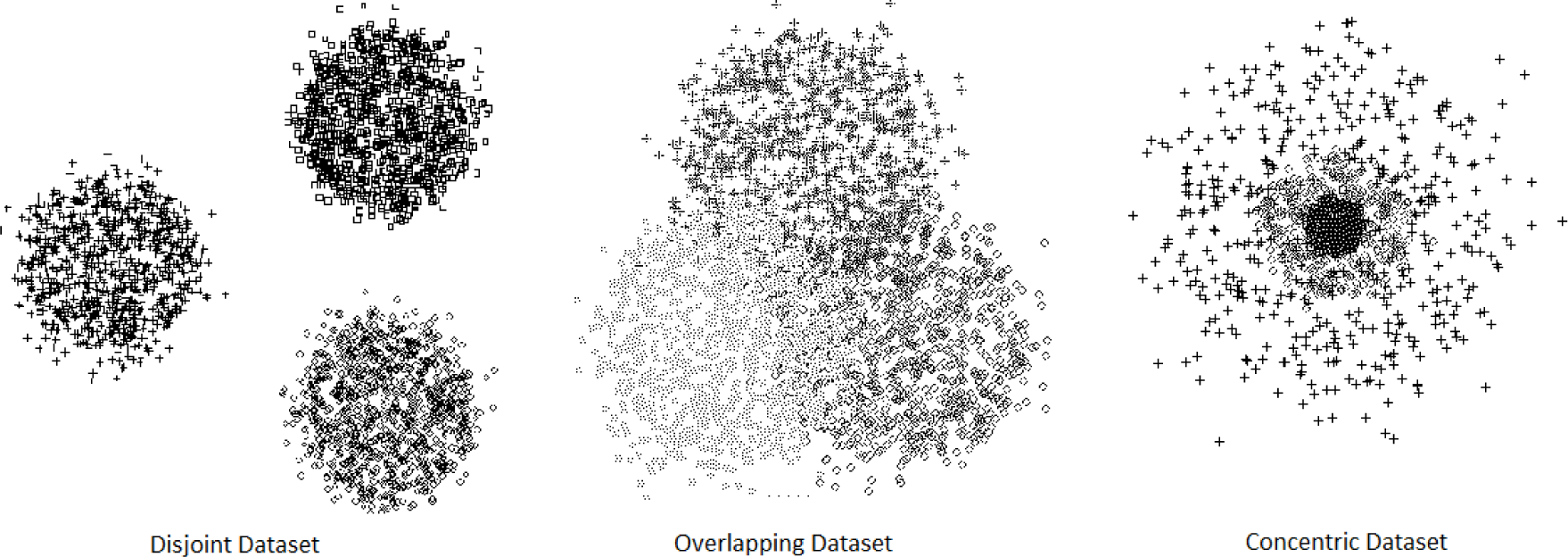
For disjoint sets, which offer no major difficulty, all four methods (k-means, fuzzy c-means, ENCLUS and CBE) perform very well relative to BC. However, when tackling partially overlapping and concentric datasets, the differences are remarkable. The information-based methods (CBE and ENCLUS) showed the best results; nevertheless, CBE was better than ENCLUS. For non-Gaussian datasets, the values of CBE and ENCLUS also outperform the other methods. When CBE is compared to ENCLUS, CBE is 62.5% better.
In conclusion, CBE is a non-supervised, highly efficient, universal (in the sense that it may be easily utilized with other quality indices) clustering technique whose effectiveness has been proven by tackling a very large number of problems (1,530,000 combined instances). It has been, in practice, used to solve complex clustering problems that other methods were not able to solve.

Acknowledgments

The authors acknowledge the support of Instituto de Investigaciones en Matemáticas Aplicadas y en Sistemas and Asociación Mexicana de Cultura A.C.

Appendix

A. Eclectic Genetic Algorithm

For those familiar with the methodology of genetic algorithms, it should come as no surprise that a number of questions relative to the best operation of the algorithm immediately arose. The simple genetic algorithm [46] frequently mentioned in the literature leaves open the optimal values of, at least, the following parameters:
  • Probability of crossover (Pc).
  • Probability of mutation (Pm).
  • Population size.
Additionally, premature and/or slow convergence are also of prime importance. For this, the EGA includes the following characteristics:
  • The best (overall) n individuals are considered. The best and worst individuals (1 − n) are selected; then, the second best and next-to-the-worst individuals (2 − [n − 1]) are selected, etc.
  • Crossover is performed with a probability Pc. Annular crossover makes this operation position independent. Annular crossover allows for unbiased building block search, a central feature to GA’s strength. Two randomly selected individuals are represented as two rings (the parent individuals). Semi-rings of equal size are selected and interchanged to yield a set of offspring. Each parent contributes the same amount of information to their descendants.
  • Mutation is performed with probability Pm. Mutation is uniform and, thus, is kept at very low levels. For efficiency purposes, we do not work with mutation probabilities for every independent bit. Rather, we work with the expected number of mutations, which, statistically is equivalent to calculating mutation probabilities for every bit. Hence, the expected number of mutations is calculated from ℓ * n * pm, where ℓ is the length of the genome in bits and n is the number of individuals in the population.
In what follows, we present the pseudocode of EGA:
Algorithm 1. Eclectic genetic algorithm.
Entropy 17 00151f13

B. Datasets

B.1. Synthetic Gaussian Datasets

To generate a Gaussian element x = [ x 1 , x 2 , , x n ], we use the acceptance-rejection method [75,76]. In this method, a uniformly distributed random point (x1, x2, …, xn, y) is generated and accepted iff y < f(x1, x2, …, xn) where f is the Gaussian pdf. For instance, on the assumption of x 2, in Figure 8, we show different Gaussian sets obtained by applying this method.
In the context of some of our experiments, X is a set of k Gaussian sets in ℜn. We wanted to test the effectiveness of our method with datasets that satisfy the following definitions:
Definition 2. Given n and k, a dataset X is a disjoint set ifCiX, it holds that CiCj = ϕi, j = 1, 2, ..k and ij.
In Figure 9, we illustrate two possible examples of such datasets for n = 2 and k = 3. The value ρ is the correlation coefficient.
Definition 3. Given n and k, a dataset X is an overlapping set ifCi, CjX, such that CiCjϕ and CiCji, j = 1, 2, ..k and ij.
In Figure 10 we illustrate two possible examples of such datasets for n = 2 and k = 3.
Definition 4. Given n and k, a dataset X is a concentric set ifCiX, its mean value, denoted by μ C i, is equal to μ C j i, j = 1, 2, ..k.
In Figure 11 we illustrate two possible examples of such datasets for n = 2 and k = 3.
We generated 500 datasets for each type (1500 total), randomly choosing the values of n and k, nU[220] and kU[215]. In Table 12, we show the parameters of this process.

B.2. Synthetic Non-Gaussian Datasets

To generate Non-Gaussian patterns in ℜn, we resort to polynomial functions of the form:
f ( x 1 , x 2 , , x n ) = a m 1 x 1 m + + a m n x n m + a 11 x 1 + a 1 n x n
Given that such functions have larger degrees of freedom, we can generate many points uniformly distributed in ℜn. As reported in the previous section, we wrote a computer program that allows us to obtain a set of 500 different problems. These problems were generated for random values of n and k (U ∼ [220] and U ∼ [215], respectively) with |Ci| = 200.

B.3. “Real World” Datasets

In order to illustrate the performance of our method when faced with “real world” problems, we selected five datasets (Abalone [77], Cars [78], Census Income[79], Hepatitis [80] and Yeast [81]) from the UCI Machine Learning repository, whose properties are shown in Table 13.
We chose datasets that represent classification problems where the class labels for each object are known. Then, we can determine the performance of any clustering method as an effectiveness percentage. The selection criteria of these datasets were based on the following features:
  • Multidimensionality.
  • Cardinality.
  • Complexity (non-linearly separable problems).
  • Categorical data.
  • Data with missing values.
Some of these features involve preprocessing tasks to guarantee the quality of a dataset. We applied the following preprocessing techniques:
  • Categorical variables were encoded using dummy binary variables [82].
  • We scaled the dataset into [0, 1).
  • In order to complete missing information, we interpolate the unknown values with natural splines (known to minimize the curvature of the approximant) [83].

C. Ensuring Normality in an Experimental Distribution

We wish to experimentally find the parameters of the unknown probability density function (pdf) of a finite, but unbounded, dataset X. To do this, we must determine the minimum number of elements M that we need to sample to ensure that our experimental approximation is correct with a desired probability P. We start by observing that a mean value is obtained from X by averaging N randomly-selected values of the xi, thus: x i = 1 N x i We know that any sampling distribution of the x i (sdm) will be normal with parameters μ x ¯ and σ x ¯ when N → ∞. In practice, it is customary to consider that a good approximation will be achieved when N > 20; hence, we decided to make N = 36. Now, all we need to determine the value of M is to find sufficient x ¯ i s ( i = 1 , 2 , , M ) until they distribute normally. Once this occurs, we immediately have the parameters μ x ¯ and σ x ¯. The parameters of the unknown pdf are then easily calculated as μ = μ x ¯ and σ = n σ x ¯. To determine that normality has been reached, we followed the following strategy. We used a setting similar to the one used in the χ2 test in which: (1) We defined ten categories di (deciles) and the corresponding 11 limiting values (vi) assuming a normal distribution, such that one tenth of the observations are expected per decile: v i v i + 1 N ( μ , σ ) 0.1, i = 0, 1, …, 9. For this to be true, we make, v0 = −5.000, v1 = −1.285, v2 = −0.845, v3 = −0.530, v4 = −0.255, v5 = 0.000 and the positive symmetrical values; (2) We calculated χ2 = ∑(oiei)2/ei for every xi, where oi is the observed number of events in the i-th decile and ei is the expected number of such events. For the k-th observed event, clearly, the number of expected events per decile is k/10; (3) We further require, as is usual, that there be at least omin = 5 events per decile. Small values of the calculated χ2 indicate that there is a larger similarity between the hypothesized and the true pdfs. In this case, a small χ2 means that the observed behavior of the x ¯ i s is closer to a normal distribution. The question we want to answer is: How small should χ2 be in order for us to ascertain normality? Remember the test χ2 is designed to verify whether two distributions differ significantly, so that one may reject the null hypothesis, i.e., the two populations are not statistically equivalent. This happens for large values of χ2 and is a function of the degrees of freedom (df). In our case, df = 7. Therefore, if we wanted to be 95% certain that the observed x ¯ i s were not normally distributed, we would demand that χ2 ≥ 14.0671. However, this case is different. We want to ensure the likelihood that the observed behavior of the x ¯ i s is normal. In order to do this, we performed a Monte Carlo experiment along the following lines. We set a desired probability P that the x ¯ i s are normal.
We establish a best desired value of χ2, which we will call χbest. We make the number of elements in the sample NS = 50. We then generate NS instances of N(0, 1) and count the number of times the value of the instance is in every decile. We calculate the value of the corresponding χ2 and store it. We thusly calculate 100, 000 combinations of size NS. Out of these combinations, we count those for which χ2χbest and there are at least omin observations per decile. This number divided by 100, 000, which we shall call p, is the experimental probability that, for NS observations, the sample “performs” as required. We repeat this process increasing NS up to 100. In every instance, we test whether p > P. If such is the case, we decrement the value of χbest and re-start the process. Only when pP, does the process end.
In Figure 12, we show the graph of the size of sample M vs. the experimental probability p that pP and oiomin for χbest (from the Monte Carlo experiment).
Every point represents the proportion of combinations satisfying the required conditions per 100,000 trials. For this experiment, χbest = 3.28. We obtained an approximation to a Gompertz model with S = 0.0023 and r = 0.9926. It has the form p = a e e b c M; where a = 0.046213555, b = 12.40231200, c = 0.195221110. From this expression, we solve for M, to get:
M b ln [ ln ( a P ) ] c
As may be observed, p < 0.05 for M ≥ 85, which says that the probability of obtaining χ2 ≤ 3.28 by chance alone is less than five in one hundred. Therefore, its is enough to obtain 85 or more x ¯ i s (3060 xi’s) to calculate μ and σ and be 95% sure that the values of these parameters will be correct.

Author Contributions

All authors have contributed to the study and preparation of the article. They have read and approved the final manuscript.

Conflicts of Interest

The authors declare no conflict of interest

References

  1. Bhattacharyya, A. On a measure of divergence between two statistical populations. Indian J. Stat. 1946, 7, 401–406. [Google Scholar]
  2. Kruskal, J.B. Multidimensional scaling by optimizing goodness of fit to a nonmetric hypothesis. Psychometrika 1964, 29, 1–27. [Google Scholar]
  3. Mahalanobis, P.C. On the generalized distance in statistics. Proceedings of the National Institute of Sciences of India, Calcutta, India, 16 April 1936; 2, pp. 49–55.
  4. Halkidi, M.; Batistakis, Y.; Vazirgiannis, M. On clustering validation techniques. J. Intell. Inf. Syst. 2001, 17, 107–145. [Google Scholar]
  5. Rokach, L.; Maimon, O. Clustering methods. In Data Mining and Knowledge Discovery Handbook; Springer: New York, NY, USA, 2005; pp. 321–352. [Google Scholar]
  6. MacQueen, J. Some methods for classification and analysis of multivariate observations. In The Fifth Berkeley Symposium on Mathematical Statistics and Probability; Le Cam, L.M., Neyman, J., Eds.; University of California Press: Berkeley, CA, USA, 1967; Volume 1, pp. 281–297. [Google Scholar]
  7. Bezdek, J.C. Pattern Recognition with Fuzzy Objective Function Algorithms; Springer: New York, NY, USA, 1981. [Google Scholar]
  8. Dunn, J.C. A fuzzy relative of the ISODATA process and its use in detecting vompact well-separated clusters. J. Cybern. 1973, 3, 32–57. [Google Scholar]
  9. Dunn, J.C. Well-separated clusters and optimal fuzzy partitions. J. Cybern. 1974, 4, 95–104. [Google Scholar]
  10. Friedman, J.; Hastie, T.; Tibshirani, R. The Elements of Statistical Learning: Data Mining, Inference, and Prediction, 2nd ed; Springer: Standord, CA, USA, 2001. [Google Scholar]
  11. Guha, S.; Rastogi, R.; Shim, K. Cure: An efficient clustering algorithm for large databases. Proceedings of the 1998 ACM SIGMOD International Conference on Management of Data, Seattle, WA, USA, 1–4 June 1998; pp. 73–84.
  12. Zhang, T.; Ramakrishnan, R.; Livny, M. Birch: An efficient data clustering method for very large databases. Proceedings of the ACM SIGMOD international Conference on Management of Data, Montreal, QC, Canada, 1996; pp. 103–114.
  13. Ester, M.; Kriegel, H.P.; Sander, J.; Xu, X. A density-based algorithm for discovering clusters in large spatial databases with noise. Proceedings of 2nd International Conference on Knowledge Discovery and Data Mining, Portland, OR, USA, 2–4 August 1996; pp. 226–231.
  14. Caruana, R.; Elhaway, M.; Nguyen, N.; Smith, C. Meta clustering. Proceedings of the Sixth International Conference on Data Mining, Hong Kong, China, 18–22 December; 2006; pp. 107–118. [Google Scholar]
  15. Das, S.; Abraham, A.; Konar, A. Metaheuristic Clustering; Springer: Berlin/Heidelberg, Germany, 2009. [Google Scholar]
  16. Milligan, G.W.; Cooper, M.C. An examination of procedures for determining the number of clusters in a data set. Psychometrika 1985, 50, 159–179. [Google Scholar]
  17. Tibshirani, R.; Walther, G.; Hastie, T. Estimating the number of clusters in a data set via the gap statistic. J. R. Stat. Soc. Ser. B 2001, 63, 411–423. [Google Scholar]
  18. Li, X.; Mak, M.W.; Li, C.K. Determining the optimal number of clusters by an extended RPCL algorithm. J. Adv. Comput. Intell. Intell. Inf. 1999, 3, 467–473. [Google Scholar]
  19. Peck, R.; Fisher, L.; van Ness, J. Approximate confidence intervals for the number of clusters. J. Am. Stat. Assoc. 1989, 84, 184–191. [Google Scholar]
  20. Yan, M. Methods of Determining the Number of Clusters in a Data Set and a New Clustering Criterion. Ph.D. Thesis, Virginia Polytechnic Institute and State University, Blacksburg, VA, USA, November 2005. [Google Scholar]
  21. Cha, S.H. Taxonomy of nominal type histogram distance measures. Proceedings of the American Conference on Applied Mathematics, Harvard, MA, USA, 24–26 March 2008.
  22. Kim, D.J. A novel validity index for determination of the optimal number of clusters. IEICE Trans. Inf. Syst. 2001, 84, 281–285. [Google Scholar]
  23. Liu, Y.; Li, Z.; Xiong, H.; Gao, X.; Wu, J. Understanding of internal clustering validation measures. Proceedings of the 10th International Conference on Data Mining (ICDM), Sydney, Australia, 13–17 December 2010; pp. 911–916.
  24. Larsen, B.; Aone, C. Fast and effective text mining using linear-time document clustering. Proceedings of the Fifth ACM SIGKDD International Conference on Knowledge Discovery and Data Mining, San Diego, CA, USA, 15–18 August 1999; pp. 16–29.
  25. Strehl, A.; Ghosh, J. Cluster ensembles—A knowledge reuse framework for combining multiple partitions. J. Mach. Learn. Res. 2003, 3, 583–617. [Google Scholar]
  26. Shannon, C.E. A Mathematical Theory of Communication. Bell Syst. Tech. J. 1948, 27, 379–423. [Google Scholar]
  27. Zhao, Y.; Karypis, G. Criterion Functions for Document Clustering: Experiments and Analysis. Available online: http://glaros.dtc.umn.edu/gkhome/node/165 accessed on 5 January 2015.
  28. Raftery, A.E. A note on bayes factors for log-linear contingency table models with vague prior information. J. R. Stat. Soc. Ser. B 1986, 48, 249–250. [Google Scholar]
  29. Rousseeuw, P.J. Silhouettes: A graphical aid to the interpretation and validation of cluster analysis. J. Comput. Appl. Math. 1987, 20, 53–65. [Google Scholar]
  30. Davies, D.L.; Bouldin, D.W. A cluster separation measure. IEEE Trans. Pattern Anal. Mach. Intell. 1979, PAMI-1, 224–227. [Google Scholar]
  31. Rendón, E.; Garcia, R.; Abundez, I.; Gutierrez, C.; Gasca, E.; del Razo, F.; Gonzalez, A. Niva: A robust cluster validity. Proceedings of the WSEAS International Conferenceon Communications, Heraklion, Greece, 23–25 July 2008.
  32. Rand, W.M. Objective criteria for the evaluation of clustering methods. J. Am. Stat. Assoc. 1971, 66, 846–850. [Google Scholar]
  33. Hubert, L.; Arabie, P. Comparing partitions. J. Classif. 1985, 2, 193–218. [Google Scholar]
  34. Graham, R.L.; Knuth, D.E.; Patashnik, O. Concrete Mathematics: A Foundation for Computer Science; Addison-Wesley: Boston, MA, USA, 1989. [Google Scholar]
  35. Glover, F. Future paths for integer programming and links to artificial intelligence. Comput. Oper. Res. 1986, 13, 553–549. [Google Scholar]
  36. Glover, F.; Laguna, M. Tabu Search; Kluwer Academic Publishers: Dordrecht, The Netherlands, 1997. [Google Scholar]
  37. Glover, F.; McMillan, C. The general employee scheduling problem. An integration of MS and AI. Comput. Oper. Res. 1986, 13, 563–573. [Google Scholar]
  38. Kirkpatrick, S. Optimization by simulated annealing: Quantitative studies. J. Stat. Phys. 1984, 34, 975–986. [Google Scholar]
  39. Kirkpatrick, S.; Gelatt, C.; Vecchi, M. Optimization by simulated annealing. Science 1983, 220, 671–679. [Google Scholar]
  40. Dorigo, M.; Blum, C. Ant colony optimization theory: A survey. Theor. Comput. Sci. 2005, 344, 243–278. [Google Scholar]
  41. Eberhart, R.; Kennedy, J. A new optimizer using particle swarm theory. Proceedings of the Sixth International Symposium on Micro Machine and Human Science, Nagoya, Japan, 4–6 October 1995; pp. 39–43.
  42. Bäck, T.; Schwefel, H.-P. An overview of evolutionary algorithms for parameter optimization. Evol. Comput. 1993, 1, 1–23. [Google Scholar]
  43. Beyer, H.G.; Schwefel, H.P. Evolution Strategies—A Comprehensive Introduction; Kluwer Academic Publishers: Dordrecht, The Netherlands, 2002; Volume 1. [Google Scholar]
  44. Fogel, L.J. The future of evolutionary programming. Proceedings of the Twenty-Fourth Asilomar Conference on Signals, Systems and Computers, Pacific Grove, CA, USA, 5–7 November 1990; 2, pp. 1036–1038.
  45. Banzhaf, W.; Nordin, P.; Keller, R.E.; Francone, F.D. Genetic Programming: An Introduction: On the Automatic Evolution of Computer Programs and Its Applications; The Morgan Kaufmann Series in Artificial Intelligence; Morgan Kaufmann Publishers: Burlington, MA, USA, 1997. [Google Scholar]
  46. Holland, J.H. Adaptation in Natural and Artificial Systems: An Introductory Analysis with Applications to Biology, Control, and Artificial Intelligence, 2nd ed; MIT Press: Cambridge, MA, USA, 1992. [Google Scholar]
  47. Rudolph, G. Convergence Analysis of Canonical Genetic Algorithms. IEEE Trans. Neural Netw. 1994, 5, 96–101. [Google Scholar]
  48. Kuri-Morales, A.; Aldana-Bobadilla, E. The best genetic algorithm I. Proceedings of the 12th Mexican International Conference on Artificial Intelligence, Mexico City, Mexico, 24–30 November 2013; pp. 1–15.
  49. Kuri-Morales, A.; Aldana-Bobadilla, E.; López-Peña, I. The best genetic algorithm II. Proceedings of the 12th Mexican International Conference on Artificial Intelligence, Mexico City, Mexico, 24–30 November 2013; pp. 16–29.
  50. Kuri-Morales, A. A statistical genetic algorithm. Available online: http://cursos.itam.mx/akuri/2006/Algoritmos%20Gen%E9ticos/2Statistical%20GA.pdf accessed on 7 January 2015.
  51. Kuri-Morales, A.; Villegas, C.Q. A universal eclectic genetic algorithm for constrained optimization. Proceedings of the 6th European Congress on Intelligent Techniques and Soft Computing, Aachen, Germany, 7–10 September 1998; 1, pp. 518–524.
  52. Abudalfa, S.I. Metaheuristic Clustering Algorithm. Ph.D. Thesis, The Islamic University of Gaza, Gaza, Palestine, 2010. [Google Scholar]
  53. Caballero, R.; Laguna, M.; Martí, R.; Molina, J. Multiobjective Clustering with Metaheuristic Optimization Technology. Available online: http://www.uv.es/sestio/TechRep/tr02-06.pdf accessed on 5 January 2015.
  54. Shelokar, P.S.; Jayaraman, V.K.; Kulkarni, B.D. An ant colony approach for clustering. Anal. Chim. Acta. 2004, 509, 187–195. [Google Scholar]
  55. Faivishevsky, L.; Goldberger, J. A nonparametric information theoretic clustering algorithm. Proceedings of the 27th International Conference on Machine Learning, Israel, Israel, 21–24 June 2010.
  56. Gokcay, E.; Principe, J.C. Information theoretic clustering. IEEE Trans. Pattern Anal. Mach. Intell. 2002, 24, 158–171. [Google Scholar]
  57. Hino, H.; Murata, N. A nonparametric clustering algorithm with a quantile-based likelihood estimator. Neural Comput. 2014, 26, 2074–2101. [Google Scholar]
  58. Jenssen, R.; Hild, K.E.; Erdogmus, D.; Principe, J.C.; Eltoft, T. Clustering using Renyi’s entropy. Proceedings of the International Joint Conference on Neural Networks, Portland, OR, USA, 20–24 July, 2003; pp. 523–528.
  59. Slonim, N.; Atwal, G.S.; Tkačik, G.; Bialek, W. Information-based clustering. Proc. Natl. Acad. Sci. USA 2005, 102, 18297–18302. [Google Scholar]
  60. Sugiyama, M.; Niu, G.; Yamada, M.; Kimura, M.; Hachiya, H. Information-maximization clustering based on squared-loss mutual information. Neural Comput. 2014, 26, 84–131. [Google Scholar]
  61. Cover, T.M.; Thomas, J.A. Elements of Information Theory, 2nd ed; Wiley: Hoboken, NJ, USA, 2006. [Google Scholar]
  62. Cheng, C.-H.; Fu, A.W.; Zhang, Y. Entropy-based subspace clustering for mining numerical data. Proceedings of the Fifth ACM SIGKDD International Conference on Knowledge Discovery and Data Mining, San Diego, CA, USA, 15–18 August 1999; pp. 84–93.
  63. Marques de Sá, J.P. Pattern Recognition: Concepts, Methods, and Applications; Springer: Berlin/Heidelberg, Germany, 2001. [Google Scholar]
  64. Duda, R.O.; Hart, P.E.; Stork, D.G. Pattern Classification; Wiley: New York, NY, USA, 2000. [Google Scholar]
  65. Haykin, S. Neural Networks: A Comprehensive Foundation, 2nd ed; Prentice Hall: Upper Saddle River, NY, USA, 1999. [Google Scholar]
  66. Gallager, R.G. Information Theory and Reliable Communication; Wiley: Hoboken, NJ, USA, 1968. [Google Scholar]
  67. Jaynes, E.T. Information theory and statistical mechanics. Phys. Rev. 1957, 106, 620–630. [Google Scholar]
  68. Deb, K. Multi-Objective Optimization Using Evolutionary Algorithms; Wiley: Chichester, UK, 2001. [Google Scholar]
  69. Snyman, J. Practical Mathematical Optimization: An Introduction to Basic Optimization Theory and Classical and New Gradient-Based Algorithms; Springer: New York, NY, USA, 2005. [Google Scholar]
  70. Thomas, G.B.; Finney, R.L.; Weir, M.D. Calculus and Analytic Geometry; Addison-Wesley: Boston, MA, USA, 1988. [Google Scholar]
  71. Censor, Y. Pareto optimality in multiobjective problems. Appl. Math. Optim. 1977, 4, 41–59. [Google Scholar]
  72. Sindhya, K.; Sinha, A.; Deb, K.; Miettinen, K. Local search based evolutionary multi-objective optimization algorithm for constrained and unconstrained problems. Proceedings of the IEEE Congress on Evolutionary Computation, Trondheim, Norway, 18–21 May 2009; pp. 2919–2926.
  73. Zitzler, E.; Laumanns, M.; Thiele, L. SPEA2: Improving the Strength Pareto Evolutionary Algorithm. Available online: http://www.kddresearch.org/Courses/Spring-2007/CIS830/Handouts/P8.pdf accessed on 5 January 2015.
  74. Steliga, K.; Szynal, D. On Markov-Type Inequalities. Int. J. Pure Appl. Math. 2010, 58, 137–152. [Google Scholar]
  75. Casella, G.; Robert, C.P. Monte Carlo Statistical Methods; Springer: New York, NY, USA, 1999. [Google Scholar]
  76. Johnson, J.L. Probability and Statistics for Computer Science; Wiley: Hoboken, NJ, USA, 2003. [Google Scholar]
  77. Abalone Data Set. Available online: http://archive.ics.uci.edu/ml/datasets/Abalone accessed on 30 December 2014.
  78. Cars Data Set. Available online: http://archive.ics.uci.edu/ml/datasets/Car+Evaluation accessed on 30 December 2014.
  79. Census Income Data Set. Available online: http://archive.ics.uci.edu/ml/datasets/Census+Income accessed on 30 December 2014.
  80. Hepatitis Data Set. Available online: http://archive.ics.uci.edu/ml/datasets/Hepatitis accessed on 30 December 2014.
  81. Yeast Data Set. Available online: http://archive.ics.uci.edu/ml/datasets/Yeast accessed on 30 December 2014.
  82. Agresti, A. Categorical Data Analysis; Wiley: Hoboken, NJ, USA, 2002. [Google Scholar]
  83. Shampine, L.F.; Allen, R.C.; Pruess, S. Fundamentals of Numerical Computing; Wiley: New York, NY, USA, 1997. [Google Scholar]
Figure 1. Example of a clustering problem. (a) Dataset X1; (b) solution for k = 2; and (c) another solution for k = 2.
Entropy 17 00151f1
Figure 2. Another clustering problem. (a) Dataset X2; (b) solution for k = 2; and (c) another solution for k = 2.
Entropy 17 00151f2
Figure 3. Feasible partition sets of X ∈ ℜ2 for k = 2. (a) Π1 and (b) Π2.
Entropy 17 00151f3
Figure 4. Representation of p ( x | C 1 ).
Entropy 17 00151f4
Figure 5. Example of the probability space of Ci in ℜ.
Entropy 17 00151f5
Figure 6. Example of the probability space of Ci in ℜ3.
Entropy 17 00151f6
Figure 7. Example of possible arrangements of a Gaussian dataset.
Entropy 17 00151f7
Figure 8. Gaussian sets in ℜ2.
Entropy 17 00151f8
Figure 9. Disjoint Gaussian sets for n = 2 and k = 3. (a) ρ = 0 and (b) ρ = 0.4, ρ = −0.7, ρ = 0.7.
Entropy 17 00151f9
Figure 10. Overlapping Gaussian sets for n = 2 and k = 3. (a) ρ = 0 and (b) ρ = 0.8, ρ = −0.8.
Entropy 17 00151f10
Figure 11. Concentric Gaussian sets for n = 2 and k = 3. (a) μ C i = ( 0 . 5 , 0 . 5 ) i and ρ = 0 and (b) μ C i = ( 0 . 5 , 0 . 5 ) i and ρ = −0.9.
Entropy 17 00151f11
Figure 12. Size of sample M vs. p.
Entropy 17 00151f12
Table 1. Unidimensional dataset.
XC
9C1
10C1
9C1
2C2
1C2
Table 2. Probability model of Π*.
XCp(x|C1)p(x|C2)
9C10.3330.000
10C10.3330.000
11C10.3330.000
2C20.0000.500
1C20.0000.500
Table 3. Probability model and the entropy of Π*.
XCp(x|C1)p(x|C2)p(x|C1)log (p(x|C1))p(x|C2)log (p(x|C2))
9C10.3330.000−0.5280.000
10C10.3330.000−0.5280.000
11C10.3330.000−0.5280.000
2C20.0000.5000.000−0.500
1C20.0000.5000.000−0.500

H(Π*)2.584
g(Π*)1.316
Table 4. Probability model and entropy of Π1.
XCp(x|C1)p(x|C2)p(x|C1)log (p(x|C1))p(x|C2)log (p(x|C2))
9C10.2500.000−0.5000.000
10C10.2500.000−0.5000.000
11C10.2500.000−0.5000.000
2C20.0001.0000.0000.000
1C10.2500.000−0.5000.000

H1)2.000
g1)3.960
Table 5. Probability model and entropy of Π2.
XCp(x|C1)p(x|C2)p(x|C1)log (p(x|C1))p(x|C2)log (p(x|C2))
9C20.0000.3330.000−0.528
10C10.5000.000−0.5000.000
11C10.5000.000−0.5000.000
2C20.0000.3330.000−0.528
1C20.0000.3330.000−0.528

H2)2.584
g2)4.059
Table 6. Average effectiveness (φ) for Gaussian datasets.
AlgorithmDisjointOverlappingConcentric
k-means0.0180.420.52
fuzzy c-means0.0170.360.51
ENCLUS0.0190.040.12
CBE0.0200.030.04

p-value < 0.05
Table 7. Performance relative to the Bayes classifier (BC) (%).
AlgorithmDisjointOverlappingConcentric
k-means0.9820.5760.475
fuzzy c-means0.9830.6360.485
ENCLUS0.9810.9600.879
CBE0.9800.9700.960

BC1.0001.0001.000

p-value < 0.05
Table 8. Average effectiveness (φ) for non-Gaussian datasets. ENCLUS, entropy clustering; CBE, clustering-based on entropy.
Algorithmμ(φ)
k-means0.56
fuzzy c-means0.54
ENCLUS0.13
CBE0.08
p-value < 0.05
Table 9. Performance relative to MLP (%).
AlgorithmPercentual Performance
k-means0.440
fuzzy c-means0.460
ENCLUS0.870
CBE0.920

MLP1.000

p-value < 0.05
Table 10. Effectiveness achieved by CBE and other clustering methods for experimental data.
SetCBEENCLUSk-MeansFuzzy c-MeansMLP
Abalone0.5960.5630.4960.5110.690
Cars0.9170.8960.6960.7120.997
Census0.8550.8120.7740.7861.000
Hepatitis0.8590.8460.7820.8110.987
Yeast0.5450.4960.4700.4860.750

Average0.7540.7230.6440.6610.885
Table 11. Performance relative to MLP.
MethodRelative Effectiveness
k-means0.728
Fuzzy c-means0.747
ENCLUS0.817
CBE0.853

MLP1.000
Table 12. Parameters of the generation process of datasets.
ParameterValue
Type of datasetDisjoint, Overlapping, Concentric
Clusters per dataset (k)U ∼ [215]
Dimensionality (n)U ∼ [220]
Cardinality of cluster (|C|)1000 elements
Maximum size of a dataset15,000 elements
Dataset per type500
Total number of problems1500
Table 13. Properties of the selected datasets.
Problem’s NameNumber of VariablesNumber of ClassesSample SizeMissing Values
Abalone843133no
Cars2241728no
Census Income14232,561yes
Hepatitis202155yes
Yeast1081486no

