1. Introduction
One of the most important contributions to the theoretical foundations of the social sciences in recent years has been the introduction of methods from physics, and particularly statistical mechanics, in order to model large scale human social behaviour. The field is vast and includes complex network theory [
1], statistical mechanics of game theory [
2], growth and creativity in cities [
3] and financial markets [
4] amongst many others. Many of these systems can be represented using the stochastic partial differential equations often studied in physics in order to understand the long term behaviour of socially structured systems [
5,
6].
The application of these techniques to economic game theory allows us to construct formal models of the simplified interactions between people when individual rewards are dependent on joint choices. The appeal of this as an approach is seen in the number of fields to which these ideas have been applied beyond the micro-economics from which it was borne: evolutionary genetics [
7]; political strategy [
8]; psychology [
9]; catastrophes [
10]; information theory of decisions [
11]; and others [
12].
One of the first and most important results in game theory is that of the Nash equilibrium [
13], where people are able to make perfect value maximising decisions in which no-one has an incentive to independently change their strategy. Equilibrium here means mutually agreeable in some carefully defined way, this notion of optimal decision making and equilibrium has been extended to that of less than perfect decisions, an aspect that is now well embedded in both the practical and the theoretical foundations of decision-making [
14].
While it is common to discuss game theory in terms of two or more people or players, we often have in mind a more general situation in which each player is replaced by two sub-populations of economic agents who make their decisions independently and based on the incentives for the choices that characterise each sub-population. To keep a concrete example in mind we imagine a highly abstract sub-population of car buyers who can choose between electric powered cars or petrol powered cars and a sub-population of energy providers who can sell either electricity through recharge outlets or petrol through traditional petrol stations.
Using this framework of non-cooperative game theory the article is divided into the following sections. Section 2 introduces the necessary notation and ideas from classical non-cooperative game theory. Readers familiar with game theory may choose to skim this section noting only the notation that will be used later. Section 3 introduces a stochastic form of game theory equilibrium called the Quantal Response Equilibrium (QRE) and two approaches to its role as an equilibrium solution are reviewed and related to the Maximum Entropy technique of Jaynes [
15]. A simple example of the Prisoner’s Dilemma is used in Section 3.1 to illustrate the basic ideas. A very useful
tracing technique will be introduced in Section 4 that will significantly aid in later analysis of equilibrium solutions. In this section we also provide illustrations of some of the more surprising properties of the QRE solution. Section 5 provides a discussion and summary of key points.
2. Game Theory
The notion of stochastic dynamics and imperfect decision-making forms the basis of the work in this article and is introduced in Section 3, but first we introduce the Nash equilibrium [
13] in which optimal (perfect, value maximising) decisions are made by economic agents. In the simplest case there are two players each of whom has two choices and their joint choices result in some form of payoff. For example in the payoff matrices shown below, Colin can choose between either the left or the right columns (
cols) and Rowena can choose between either the top or the bottom
rows, each player then receives the payoff as shown in the matrices:
The goal of game theory is to model the choices adopted by players based on specific variations in the concept of “rational choice”. For example Nash described a type of rationality in which each player can choose a distribution over their options, i.e., pc(left) and pc(right) are probabilities over col’s two choices and pr(top) and pr(bottom) are probabilities over row’s choices. Each player then seeks to independently choose the probabilities that maximise their expected payoffs given by:
where E(·) is an expectation function over the indexed joint strategies i, j and
and
are entries in the payoff matrices. Each player then maximises their expected utility using probabilities
and
:
such that neither player can increase their expected utility by unilaterally changing their strategy. Two players who maximise their expected utilities in this fashion will arrive at a Nash equilibrium. Pure strategies are those in which col (for example) plays with certainty one of their choices, e.g. pc(left) = 1. A mixed strategy is one in which players choose using a distribution different from a pure strategy. While the Nash equilibrium concept is not the only form of rationality that players may follow it has been a cornerstone of modern micro-economic game theory since it was first proposed. An alternative called the Quantal Response Equilibrium will be introduced later.
Instead of using the probabilities as shown above, it will be useful to frame what follows in terms of a behavioural strategy for each player, Qr,Qc ∈ [−1, 1], given by the mappings:
and
. This allows us to express the expected utilities in the following slightly more compact fashion. First construct four functions (explained next) for each player based upon their respective utility matrices in matrices 1 where x ∈{r, c}:
The expected utilities can then be expressed as a polynomial in player strategies Qr and Qc composed of an intrinsic term, a self-interaction term, an influence term from the other player and a joint interaction term:
We will also make use of the conditional expected utility, this is the expected payoff a player will earn given that they choose one of their strategies, denoted sr and sc:
We will also use the difference in the conditional expected utilities for two choice games, given by:
In the next section we introduce the Quantal Response Equilibrium, an alternative equilibrium containing the Nash Equilibrium as a limiting case.
3. The Quantal Response Equilibrium for Game Theory
While the Nash equilibrium has played a key role in modern game theory, it has a number of shortcomings when used to describe the observed behaviour of decision-makers [
9,
16] and this has motivated the development of alternative notions of equilibrium. McKelvey and Palfrey proved [
17] that there is an alternative equilibrium available in game theory that contains the Nash equilibrium as a special case and called it the Quantal Response Equilibrium (QRE). Their approach used methods from differential topology and Brouwer’s fixed point theorem in order to prove their key results. In economic terms this is not a very satisfying approach so instead we motivate our use of the QRE via an economic justification of the maximum entropy principle (MaxEnt) [
15] that can then be used to derive the QRE.
We begin with the entropy of a probability distribution
p over the
i discrete states of a system:
S(
p)= −∑
i p(
i) ln(
p(
i)) which has often been interpreted as a measure of the spread or
diversity of
p. This interpretation was discussed at least as early as 1975 in economics [
18] and it is a well established measure in ecology [
19] in which understanding the biodiversity of an ecological system is important. In combination with other desiderata [
20] the entropy is the unique function that has the property that when it is applied to independent subsystems the sum of the parts is equal to the whole. For example if a system can be partitioned into two independent subsystems
A and
B (as we do below) with probability distributions
p and
q with joint probabilities
pq, then
S(
A+
B)=
S(
A)+
S(
B) and
S(
pq)=
S(
p)+
S(
q), we expand on this next.
The
measure of diversity interpretation of entropy implies that maximising
S(
p) is equivalent to maximising the diversity of an economy, often thought to be an economically sound goal [
21]. However, maximising the entropy without constraints results in a uniform distribution and in economics this would be equivalent to assuming there are no resource constraints or there are no incentives to produce or purchase one product rather than another, neither interpretation is economically reasonable. Further, given the subsystem additivity property of the entropy, any “localised” maximisation of an independent sub-system’s diversity contributes additively to the whole system diversity, so aggregated local maximisation results in a global optimum. Once constraints are included in an economic model, then maximising the economic diversity subject to (mean valued) resource constraints is equivalent to the MaxEnt procedure, and hence our use of the technique outlined next (this approach follows [
10,
22]).
The MaxEnt technique applied to game theory begins with the notion of finding the distribution
, x ∈{r, c}, that maximises the entropy S(px)= −∑ipx(i) ln(px(i)) of each player’s distribution. For a 2 player game in which each player has k discrete choices from which to select, each player individually maximises the entropy associated with the distribution over their choices:
subject to the constraints:
Such a constrained optimisation problem can be solved by forming the Lagrangian
![Entropy 16 05102f8]()
(
px)and then solving the stationary solutions ∂
{px}
![Entropy 16 05102f8]()
(
px)=0 for
px in the following way:
where the
term enforces the normalisation constraints and the last step is the substitution of
Equations (12),
(13) into
Equation (20). The result of both players maximising their respective entropies independently of each other is the QRE,
Equation (21), which is a globally optimal solution as the joint probabilities of
r and
c choosing strategies
i or
j is:
pr,c(
i, j)=
pr(
i)
pc(
j), which is the assumption of independence of non-cooperative game theory. This should be compared with the Nash equilibrium in which individuals independently maximise their utilities, not their entropies, via the expected utility functions. The difference can be interpreted in terms of individuals vs. large populations, discussed below in terms of the Fokker–Planck equation.
Equation (21) can be rewritten in the form:
This is the hyperbolic behavioural form of
Equation (21) expressed in the notation introduced in
Equations (6)–
(15). The differences between the forms of
Equation (21) and
Equations (22) and
(23) are a matter of emphasis:
Equation (21) focuses on the expected utility and how that results in biasing one choice over the other,
Equations (22) and
(23) emphasise the strategic interaction between the players, how one player’s choice influences and interacts with the other’s.
The QRE has been used as a model of bounded rationality [
23] as variation in the (
βr,βc) pair can each separately and independently vary from ∞ (perfect rationality: when (
βr,βc) = (∞
, ∞) the Nash equilibria are recovered), through 0 (strategic indifference: when (
βr,βc) =(0
, 0) the players play uniformly across strategies) to −∞ in which case players choose strategies that harm their expected utilities. With this range of parameters, the
β term describes the
rationality [
23] or even the
persona [
24] of each player. In this sense it can be thought of as a psychological parameter that mediates the decision-making process between the accumulation of information regarding the game and the behavioural outcome
Qx. It should be emphasised that every (
βr,βc) pair of
Equations (22) and
(23) results in an equilibrium and variation of these parameters results in another equilibrium point. Even in the simplest case of two players and two choices, there is the possibility of non-trivial results; the following sections discuss some interesting examples. Empirical evidence for the QRE as a model of individual choice can be found in the original McKelvey and Palfrey paper [
17] as well as in 2×2 games such as the matching pennies game and its generalisations [
25].
There are at least three ways in which the QRE can be derived, the original approach of McKelvey and Palfrey and MaxEnt have already been discussed and these are often specifically interpreted as choice models for individual economic agents. The third is based on the fixed point solution to a Fokker–Planck equation (FPE) phrased in terms of stochastic partial differential equations applied to entire populations of incentivised agents [
26]. The interest in this model comes from the fact that it is based on a very large number of individuals interacting with each other stochastically over time, very much like an idealised economy, see for example the body of work by Traulsen
et al. in finite populations [
26–
28] and Helbing [
29–
31]. The FPE is an important stochastic partial differential equation that has been used extensively in the social and natural sciences [
32]. It describes how a population’s probability distribution over possible states changes over time. The significance of the QRE as a behavioural model of collective choice dynamics comes from the equivalence of the MaxEnt result to the stationary solutions of an equivalent FPE. Plastino and Plastino [
33] proved this equivalence for mean valued constraints (such as the expected utility of game theory). The stochastic dynamics of these evolutionary systems have been studied in a variety of different ways, see for example Helbing [
34], Sato et al. [
35] and Traulsen
et al. [
26]. Behavioural evidence has also been found for the mapping of the stationary solutions of the Fokker Planck equations to the QRE for large numbers of individuals playing games, see for example [
36].
A few comments are in order to provide an interpretation of the
β parameters of the QRE that is consistent with the use of the QRE in the context of large populations of decision-makers. As mentioned earlier, this parameter has variously been interpreted as a “rationality” parameter or a “persona” parameter and has also been interpreted as a “social temperature” parameter [
6] due to an analogy with the Boltzmann distribution used in statistical thermodynamics. As
β → 0 decision-makers perceive the value of two options (value
A > B) to be more closely related as
β(
A −
B) → 0 and
whereas as
β → ∞ then
β(
A −
B) → ∞ and
p(
A) → 1,
p(
B) → 0. This is the distinction made by the QRE: small differences in utility can be made arbitrarily large or small through variation in the
β values, and this can be thought of as decision-makers being plastic in how well they can distinguish between the relative merits of their choices. As such, when differences in perceived utility are reduced, there is greater statistical variation in the choices made by decision-makers than if the perceived differences are very large. From an economic perspective taxes are a candidate mechanism by which
β increases or decreases the relative merit of different choices [
22]. To compare this with similar mathematical models of an individual’s perceptual psychology [
37,
38],
β would vary an individual’s perceptual accuracy in distinguishing between two ambiguous visual or auditory signals,
β being directly related to the expected perceptual error in the resultant decision the perceiver makes.
From this perspective, there is good reason to suggest that evaluative decision-making, be it perceptual or economic, in individuals and across populations can be modelled using stochastic evolutionary equations of the Fokker–Planck type and that this is equivalent to maximising the entropy of the distribution over choices. This provides support for the more general notion that a two player, two choice QRE framework can be interpreted as the equilibrium states of the stochastic time evolution of a two sector economy in which each sector chooses independently (no collusion) between two options. To use the example from the Introduction: One population would be a large number of car buyers choosing the power source for their cars and the other would be a large number of energy suppliers choosing which type of fuel to supply.
Next we illustrate the QRE and how variations in behavioural parameters (the β terms) moves the QRE through the space of equilibrium solutions.
3.1. Quantal Equilibrium Paths: Prisoners’ Dilemma
The Prisoners’ Dilemma is a quintessential example of the counter-intuitive results that are possible in game theory. The story of the game is that two criminals are picked up for the same crime and placed in two separate cells so that they cannot communicate and both suspects are offered the same deal: If you both choose to remain silent as to who committed the crime both suspects will get 1 year in jail, if one accuses the other while they in turn claim innocence, the accuser goes free and the accused receives a 3 year jail term, but if they both accuse each other of the crime they will each receive a 2 year jail term. The situation is depicted in the payoff matrices (
24) where left or top = silence (
Qx = −1), right or bottom = accusing the other person (
Qx = +1):
The expected utilities for the two players are:
and
, i.e., tilted planes. Note that there is no joint interaction term: fr,c(Ux)=0 and the intrinsic utility is that of a hostile environment: fi(Ux)= −1.5 so that if both players played uniform strategies: Qx =0, the expected utility would be negative. Both players have an incentive to change their behaviour Qx to accuse the other person:
, no matter what the other person actually does. As a result both players accuse each other and a sub-optimal equilibrium is achieved for both players (they both receive 2 year jail terms rather than 1 year terms if they had both remained silent). This is clear from the expected utilities, as row increases Qr this in turn increases row’s negative contribution to col’s expected utility by a factor of two, likewise as col increases Qc col’s negative contribution to the expected utility of row increases by a factor of two. The net effect is that each player drives the other to the position of mutual accusation because that is the direction of the utility gradient for changes in their respective behavioural strategies. Note that this path is not itself a path through equilibrium solutions, the only equilibrium is the Nash equilibrium at the end of this path where Qx =1 (px(accuse) = 1) for both players.
The equivalent analysis for the QRE gives a similar result, except that parametric variations result in paths that remain in equilibrium.
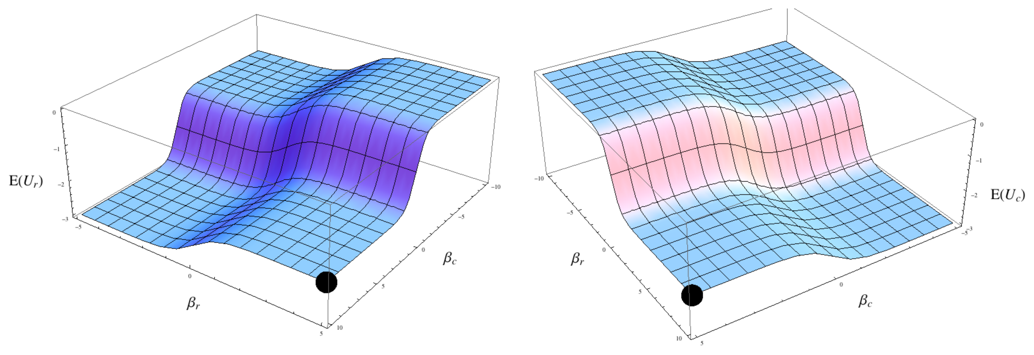
Figure 1 shows the expected utility to both prisoners in the Prisoner’s Dilemma when the player’s strategies are in equilibrium (in terms of the QRE) with each other, parameterised in terms of
βx:
Qr = tanh[
βr] and
Qc = tanh[
βc]. Substituting these values into the expected utilities and differentiating with respect to
βx:
So the players still have an incentive to increase their respective βx terms and will ultimately arrive at the original Nash Equilibrium of Qx =1, except that now the path they traverse in arriving at the point is a path through equilibrium solutions to the QRE. In this game the QRE is little different in practical terms from conventional game theory except that sub-rational equilibria, i.e., noisy and not perfectly optimising, can be described as a continuous, smooth surface parameterised by a psychological variable. It is not always so simple though as shown in the next example.
3.2. The QRE and the non-linear effects of group interactions
One of the most important contributions to the theoretical foundations of the social sciences in recent years has been the introduction of methods from physics, and particularly statistical mechanics, in order to model large scale human behaviour. Amongst the many popular models the canonical 2-D Ising model and its mean field approximation have been rigorously studied as an analogy to social interactions [
6]. In such systems, just as in the present work, it is the stationary states of the system that are often most important in the analysis. For the 2-D Ising model there is an approximation to the true equilibrium called the mean field approximation. It is a self-consistent equation of the form [
39]:
where
β is the inverse temperature of the system,
α is a shape parameter and
h is a field extrinsic to the system, e.g. an external magnetic field that is constantly perturbing the system. This system has a very distinctive set of
Q values that solves
Equation (29) for a given set of
β and
h values as shown in
Figure 2 (
α =1).
The QRE (
Equations (22) and
(23)) can be identified directly with
Equation (29) in the following way: define
βr =
βc ≡
β and the utility matrices (
1): U
r ≡ transpose[
Uc]. Now instead of having two different types of agents in the system each with their own
βr and
βc values and their own individual utilities we have only one type with discriminability
β and universal incentives. Then the identity
Qr =
Qc ≡
Q holds and:
where
x is interchangeable with either
r or
c. So when the players have the same discriminability parameter
β and equivalent payoff matrices the QRE reduces to the form of the mean field approximation of the Ising model, with a non-linear term due to the players self-interaction. The significance of this lies in the role of the Ising model (and it’s approximations) as a representation of social interactions between homogeneous agents [
6]. Also see Rosser [
40] for an interpretation of this model in terms of economics. The QRE might then be interpreted as a generalisation of
equation 29 as the mean field model of interacting agents in which one part of the population is different from another, further generalisations to many different types of agents in a population interacting in different ways strongly suggest themselves.
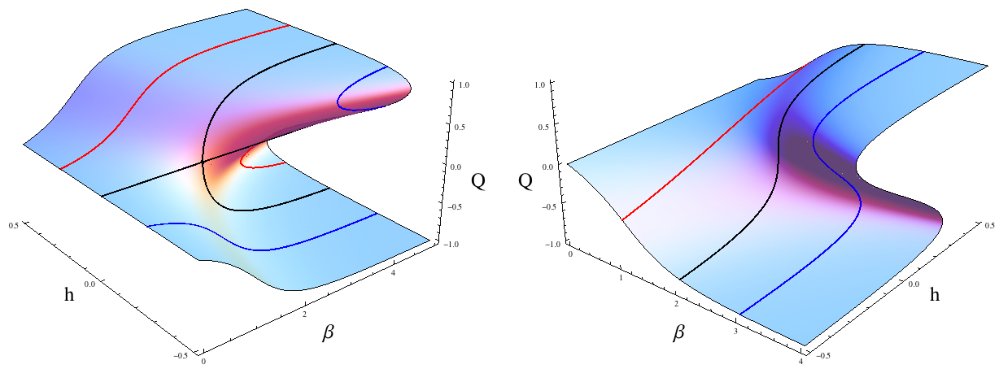
Figure 2 shows some of the most important characteristics of the mean field model. The left plot shows contour lines for fixed
β values and varying
h values where
h is often interpreted as the strength of the
social field influencing the overall orientation of the system, it is an extrinsic field that constantly perturbs the system in one direction or the other (either the
Q =1 or
Q = −1 direction) and
h of
Equation (29) is comparable to
fx(
Ux) of
Equation (32). The red and blue contours illustrate the mean field equivalent of the principal branches (see Section 4) while the black contour shows a pitchfork bifurcation that is known to be a second order phase transition [
39]. The right plot illustrates variation in the
β parameter for three different values of the social field
h. For these different values the system transitions from low
h to high
h (
i.e., constant monotonic increase) in three distinctive ways; smoothly (red curve), rapidly but still maintaining contact with the equilibrium surface (black curve) or discontinuously where the system suddenly jumps from one surface to the other as
h smoothly increases (blue curve).
These systems have been studied extensively but new results still appear regularly [
41]. The continuing interest in such models is due in part to the fact that these different types of non-equilibrium transitions in the system as parameters vary are all hallmarks of real systems in which coupled elements dynamically interact with one another. In the mean field Ising model it is possible to navigate the entire equilibrium surface
without departing from the equilibrium surface, there is always a joint change in
h and
β that can avoid a so-called tipping point (described in the next section). In this sense the strategic space can be thought of as smoothly connected.
A key aspect of the QRE though is that there are a number of important macroscopic properties of the QRE surface, notably the appearance of unavoidable tipping points and the dangerous erosion of equilibrium islands (also described in the next section) that are lost if we were to use
Equation (29) as an approximation to a non-homogeneous population for which the QRE of
Equations (22)–
(23) are the equilibrium solutions. Some of these properties have only recently been explored [
10] and so the following section introduces some of these so far unexplored properties as a function of the underlying system parameters.
4. Quantal Equilibrium Paths: Perturbed Cooperation and the principal branch of the QRE
This work focuses on the
structural instabilities of equilibrium solutions in stochastic systems. This issue is closely related to the Catastrophe Theory of Thom from the 1960’s, itself an extension of the work on singularity theory of Whitney, in which the principal object of study is the discontinuous or qualitative change in the properties of a system: “
[W]hile Newtonian theory only considers smooth, continuous processes, catastrophe theory provides a method for the study of all jump transitions, discontinuities, and sudden qualitative changes” [
42]. However, in its original formulation Catastrophe Theory only addressed deterministic systems, it was not until Cobb [
43] and more recently Wagenmakers
et al. [
44] that these ideas could be translated to the stochastic systems such as those considered here. With this notion of
Catastrophe Theory instabilities this work examines stochastic systems for which qualitative (disruptive) regime shifts occur as a function of the smooth variation in parameters.
In order to illustrate some of the more unusual results that are possible with equilibrium solutions to the QRE, the following examples will focus on a perturbed game matrix given by:
and the expected utilities:
where
δr =
δc =0 recovers
E(
Ux)=
QcQr. The QRE fixed points change as a function of the
βx terms, plots of these equilibrium surfaces in terms of
βr and
βc will be used to qualitatively illustrate significant outcomes in social interactions. Substituting the utilities from table (
33) into
Equations (6)–
(9) we find:
and
and the QRE is:
The QRE has an important characteristic called the
principal branch as illustrated in
Figure 3, this is a unique smoothly connected continuation from the origin
βrow =0 where there is only a single fixed point (
βcol = constant) to the perfect rationality solution as
βrow →∞ (alternatively
βcol →∞ and
βrow = constant), the existence of a principal branch is proven in McKelvey and Palfrey [
17] based on the earlier work of Harsanyi [
45] and the Nash Equilibrium achieved as both
βrow and
βcol →∞ is called the
limiting logit equilibrium of the game.
By changing matrices (
33) via the
δr and
δc terms in different ways the response of the system to mild parametric perturbations can be studied.
Figure 4 shows the positive
βx quadrant for a range of values of
δr =
δc where the distinctive separation (bifurcation) of equilibrium surfaces occurs in a generalised fashion (the left and right plots of
Figure 4) to that which is studied in mean-field models of social interactions [
6].
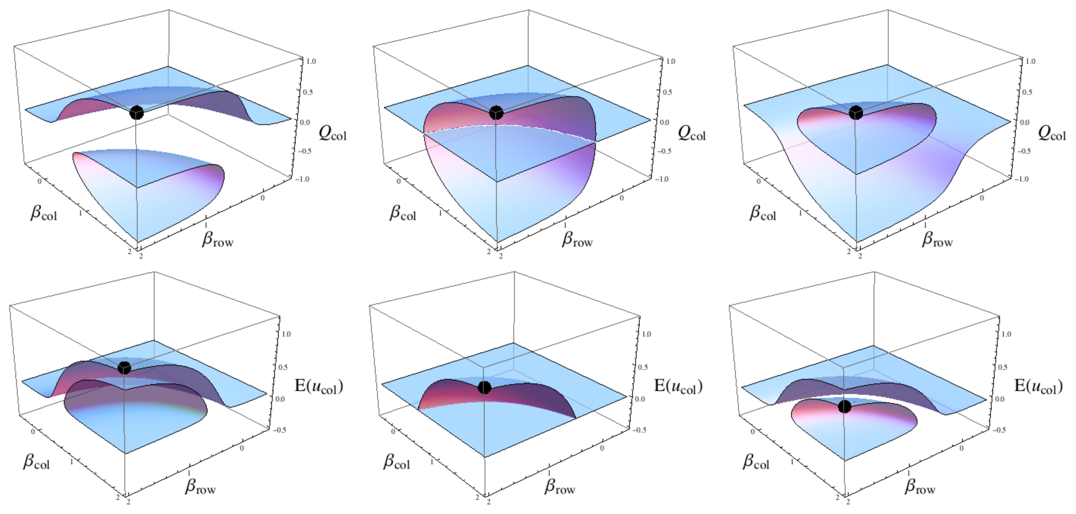
4.1. The stranding of sub-optimal strategies on equilibrium islands
Figure 4 has three plots of the equilibrium
Qr and
Qc for the following three cases of the QRE based on tables (
33):
The
δx terms can be interpreted as a mutual deterioration of the joint strategy {
B, R} in table (
33) as both
δ values decrease from positive to negative values. To continue the economic example of fuel for cars, this can be thought of as both petrol powered cars and petrol as a fuel becoming more expensive relative to the alternative of electric powered cars and supplying consumers electricity at outlets for their cars. As petrol prices at gas stations increase and manufacturing costs increase (for example through increased shipping and transport costs of raw materials due to more expensive petrol and diesel), both manufacturing petrol powered cars and buying petrol to power those cars becomes more expensive, thereby decreasing the utility of this solution to both market sectors.
The true threat is not in the actual changes in price though, seen as drops in the expected utilities shown on the bottom row of
Figure 4. The true threat is in how the previously good strategy of petrol cars and petrol fill up stations, where variation in
β values (e.g. tax rates for each market sector [
22]) cannot result in the system passing through a tipping point (left plot 4) and how this changes as this previously good strategy becomes stranded on an isolated island where moving around the strategy space can suddenly become very risky as passing over a tipping point becomes a real possibility (right plot 4). Initially this is a good approximation to a globally optimal strategy (the expected utility in the lower plot is highest for that particular
β pair) and the strategy lies on the principal branch for both
βrow and
βcol. As
δ decreases the previously good strategy is now isolated from the origin (in the right plot) and so is no longer on the principal branch for either player and the expected utility in the lower plot is no longer optimal for this
β pair.
4.2. The instability of fixed strategies located on equilibrium islands
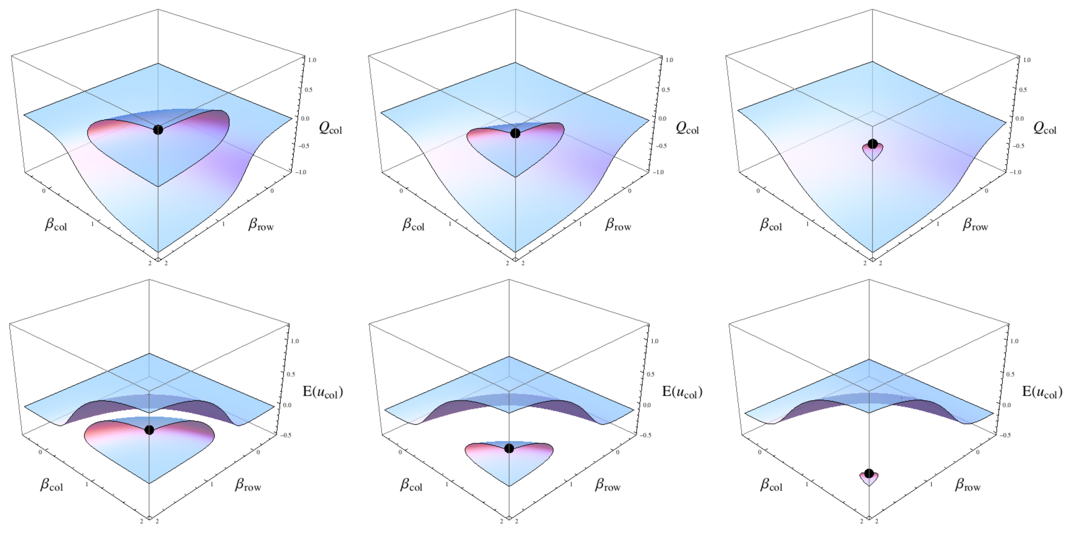
Taking the previous example of strategic islands as the starting point, we next consider what happens if the utility for the chosen strategy continues to deteriorate. This is illustrated in
Figure 5 in which the
δr =
δc perturbations to the utilities continue to decrease. If the original
β pair remains fixed at
βr =
βc =2 the bifurcation region expands towards the given strategy and eventually overtakes it, forcing the economy through a tipping point even though the
β values remain fixed.
It may be possible to try and “outrun” the encroaching bifurcation by adjusting the
β parameters (the island in
Figure 5 is only receding out of the frame of the plot) in order to try and stabilise the strategy, for example by providing tax incentives to both market sectors and thereby offsetting the increasing costs of each strategy. However, the utility of the strategy they would be pursuing is progressively decreasing and the lower the utility of their strategy becomes, the larger the ultimate strategic crash will be. This can be seen by considering
Figure 4 again, as
δr =
δc → 0 the gap between the two surfaces decreases, eventually reducing to zero when
δr =
δc =0. If the direction of change in these
δ terms is reversed the opposite effect is observed, the gap between the surfaces increases and consequently the tipping point becomes more significant the further the chosen strategy deteriorates.
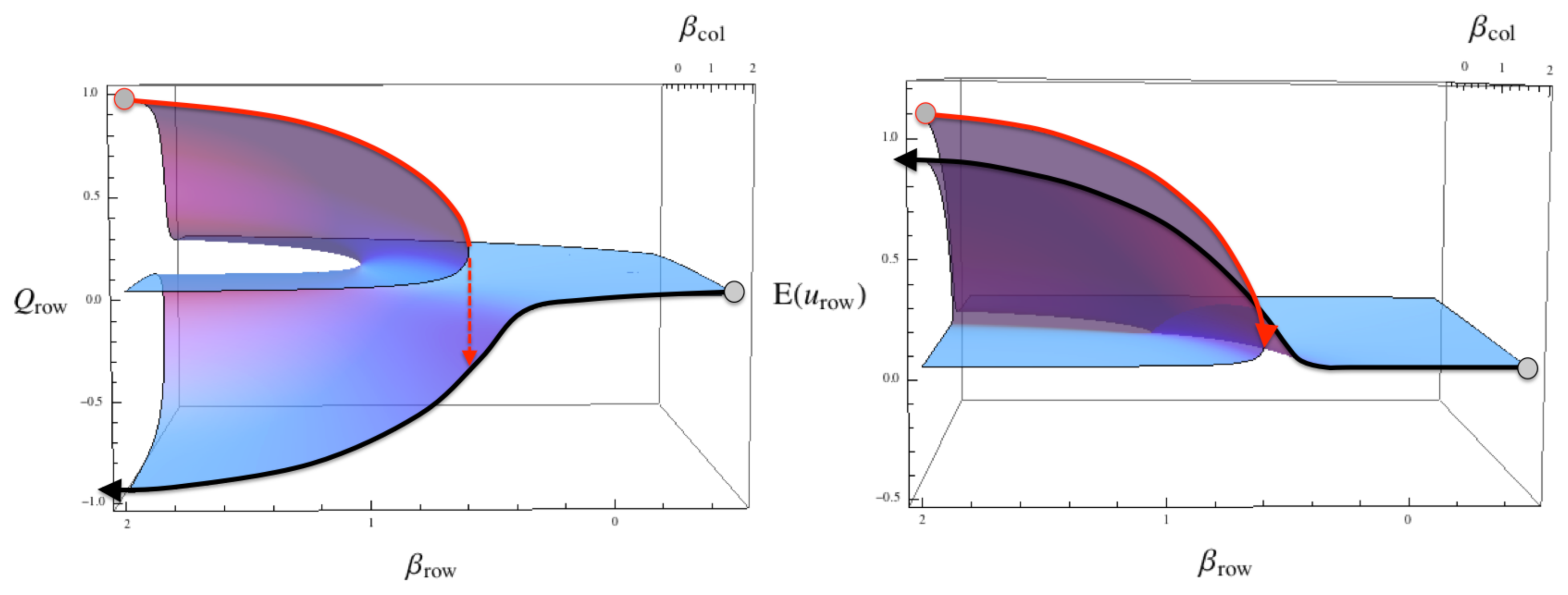
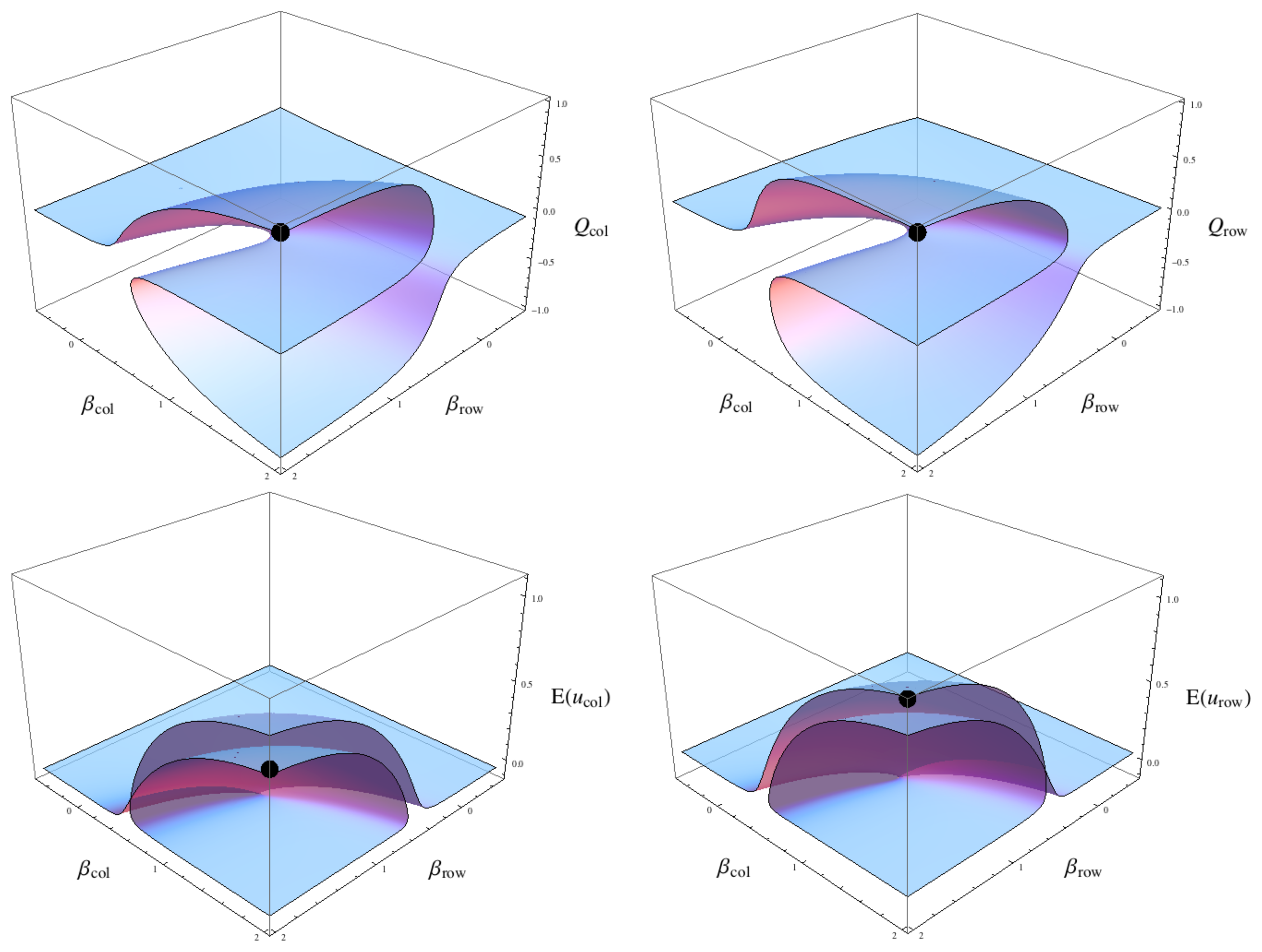
4.3. Intermingling of optimal and sub-optimal strategies via selective incentive variation
Again we consider a given equilibrium solution for a
β pair as illustrated in
Figures 6 and
7 by black dots. In this case we now selectively perturb the different utility matrices and another topological variation in the QRE surfaces can be shown, this time the equilibrium surfaces for the two
Q values are twisted in a very unusual fashion. Here, the equilibrium point of
βr =
βc ≃ 2 and
Qrow =
Qcol ≃ 1 is the optimal (for the given
β pair) for
row but it is sub-optimal for
col. This is shown in the bottom row of plots of the two expected utilities.
This result is to be expected given the structure of the utility matrices where the different δ values preferentially favour one strategy over another, but how this is then translated into a smoothly connected surface of strategies is quite surprising. Note that any tipping point in Qcol is also a tipping point in Qrow for some continuous variation in the β pairs. A consequence of this is the inter-folded aspect of the utility surfaces, E(ucol) shows an intersection between the equilibrium utility surfaces along the βc axis whereas the E(urow) shows an intersection in the utility surfaces along the βr axis. The intersection of course represents equivalent utility values where the corresponding Q values are very far apart in the strategy space, a surprising and perhaps even a counterintuitive result of the QRE.
We can also use the McKelvey and Palfrey tracing procedure for the principal branch in order to understand some of the properties of this equilibrium surface. Setting
βc =2 and allowing
βr to vary smoothly from 0 to 2 the principal branch of
row results in
Qcol ≃ −1 in the
βr → ∞ limit. Alternatively, setting
βr =2 and allowing
βc to vary smoothly from 0 to 2 the principal branch of
row results in
Qrow ≃ +1 in the
βr → ∞ limit, clearly the principal branch of one player does not correspond to the principal branch of the other player in the large
β limit. This necessitates the inter-folded nature of the utility surfaces discussed above, fixing
βr =2 and allowing
βc to vary from 0 to 2 we see in the top two plots of
Figure 6 there is a smooth path in the equilibrium surfaces for both
Qcol and
Qrow terminating at
βr =
βc =2.
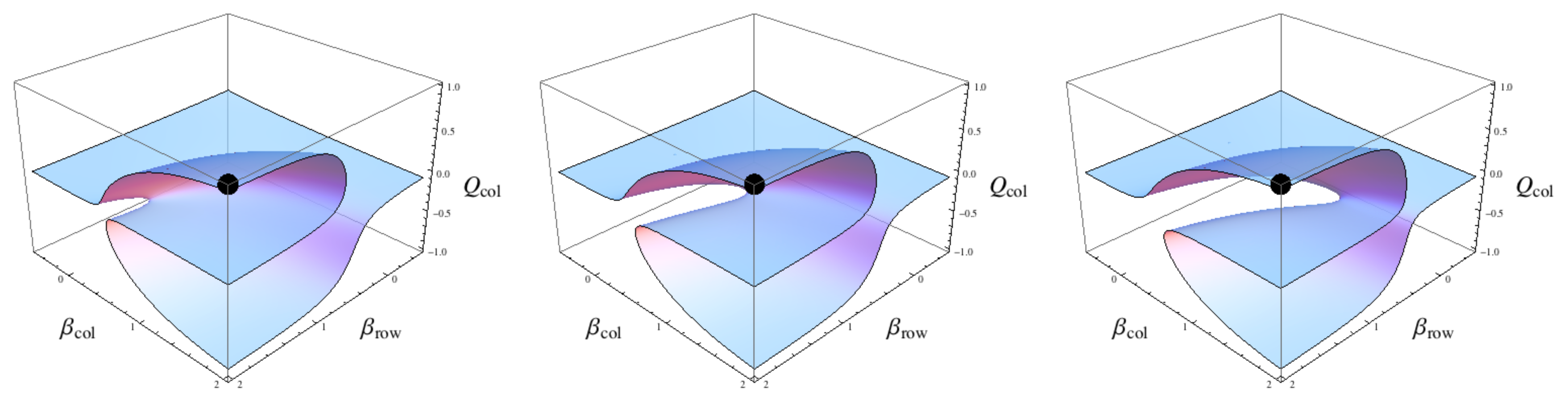
Finally, in
Figure 7 is illustrated the effect of perturbations that are due to relatively minor variations in
Figure 6. In previous work [
10] a model was developed whereby differentially “nudging” the
β parameters would enable an economy to be shifted past tipping points without necessarily adjusting the underlying incentive structure. In this example the alternative is shown whereby we ask the question: assuming
βr =
βc → 0 then what necessary changes to the incentive structure would sufficiently distort the topology of the QRE such that a tipping point could be averted? As shown in
Figure 7 the incentives can readily change the location of the tipping points such that a constant and equal variation in the
β parameters would not result in the system passing through a tipping point.
5. Conclusions
This article has focused on the qualitative features of the Quantal Response Equilibrium, an economic model used to represent imperfect economic decisions made in a social context. The emphasis has been on the “tipping points” of this model because of the incredible impact such discontinuous transitions can have on economies and society in general [
46]. Tipping points are a useful model of financial market crashes; economic depressions; and catastrophic climate change. So it is important that the possible mechanisms by which these tipping points can come about be modelled and studied when we consider the evolution of our social, economic and natural worlds, interconnected as they are.
There are three key findings that have not, at least within the framework of game theory, previously been examined as consequences of the QRE and boundedly rational decisions across an economy. The first is that the changing environment can shift a previously good strategy for two populations of decision makers to a sub-optimal outcome for both populations. This occurs when a previously good strategy has a progressively deteriorating utility. Moreover, this strategy can become isolated from the rest of the strategy space in the sense that other regions, and in particular better strategic regions, are cut-off such that they are not smoothly attainable from the current strategy.
To use the car fuel analogy, a population that buys a majority of petrol powered cars when petrol prices are low and electricity supplied for cars is expensive is an economically sound strategy. But as the cost of petrol increases while the supply of cheap electricity to fuel stations increases, then what was previously a good strategy (petrol cars and petrol stations) may become sub-optimal compared to electric cars and electric fuel stations. In order to achieve this better strategy though it may be the case that the car and energy sectors need to pass through a tipping point where both industry sectors suddenly collapse to a new equilibrium of electric cars and electric power outlets given that the previous equilibrium is not sustainable. The result could be the sudden under-utilisation of resources such as highly trained staff and manufacturing facilities while at the same time leaving industries technologically unprepared to produce new cars and fuel them, despite this being the better strategy. By far a smooth transition from one economic strategy to another is the better outcome.
The second significant finding is closely related to the first: even if the current strategy is maintained, further degradation in the utility of the existing strategy may result in the equilibrium strategy “evaporating”, leading to a different tipping point not produced by trying to navigate the space of equilibrium solutions but instead caused by the decreasing quality of the current strategy through a progressively degraded utility of that strategy.
The third significant finding is that different changes in the underlying incentive structures result in different outcomes in terms of whether or not the existing strategy is optimal or sub-optimal. The analogy in the car industry example is that one industry is preferentially incentivised over another. In this case we can imagine that oil might become more expensive to extract and transport reducing the overall profitability of petrol stations whereas the price of petrol powered cars might be subsidised through a government intervention program, resulting in cheaper petrol cars relative to electric cars. The result can be a sub-optimal outcome for the energy sector but an optimal outcome (perhaps artificially so) for the car industry.


 (px)and then solving the stationary solutions ∂{px}