Density Reconstructions with Errors in the Data

Abstract
: The maximum entropy method was originally proposed as a variational technique to determine probability densities from the knowledge of a few expected values. The applications of the method beyond its original role in statistical physics are manifold. An interesting feature of the method is its potential to incorporate errors in the data. Here, we examine two possible ways of doing that. The two approaches have different intuitive interpretations, and one of them allows for error estimation. Our motivating example comes from the field of risk analysis, but the statement of the problem might as well come from any branch of applied sciences. We apply the methodology to a problem consisting of the determination of a probability density from a few values of its numerically-determined Laplace transform. This problem can be mapped onto a problem consisting of the determination of a probability density on [0, 1] from the knowledge of a few of its fractional moments up to some measurement errors stemming from insufficient data.1. Introduction
An important problem in many applications of probability is the determination of the probability density of a positive random variable when the information available consists of an observed sample. For example, it can be either an exit time or a reaction time, the accumulated losses or accumulated damage, and so on. A standard technique, related to a variety of branches of analysis, consists of the use of the Laplace transform. However, sometimes, such a technique may fail, because the transform cannot be determined, as in the case of the lognormal variable. In this regard, see the efforts in [1] to determine the Fourier-Laplace transform of the lognormal variable. One is then led to search for techniques to invert a Laplace transform from a few of its values determined numerically. Additionally, that is the reason why we chose to use a sample from the lognormal as data to test the methods that we propose.
To state our problem: we are interested in a method to obtain a probability density fS(s) from the knowledge of the values of the Laplace transform:
To be specific, the positive random variable S may denote the severity of some kind of losses accumulated during a given time interval, and the density fS(s) is the object that we are after. Due to the importance of this problem for the insurance industry, there has been quite a large amount of effort devoted to finding systematic ways to compute fS(s) from the knowledge of the ingredients of some model relating the S to more basic quantities, like the frequency of losses and individual severities. See [2], for example, for a relatively recent update on methods to deal with that problem.
We should mention at the outset that if the Laplace transform E[e−αS] were known as a function on the positive real axis, a variety of methods to determine fS exist. Among them, the use of maximum entropy techniques that bypass the need to extend the Laplace transform into a complex half-plane. The standard maximum entropy (SME for short) method to solve this problem is simple to implement. See [3] for a comparative study of methods (including the maximum entropy) that can be used to determine fS when E[e−αX] can be computed analytically. By the way, there, we showed that with eight fractional moments (corresponding to eight values of the Laplace transform), we could obtain quite accurate inversions. That is the reason why we consider eight moments in this paper.
However, in many cases, E[e−αS] has to be estimated from observed values s1, …., sN of S, that is, the only knowledge that may be available to us is the total loss in a given period. It is at this point where errors come in, because in order to determine μ(α), we have to use the random sample and average over it. If we were somehow determining μ(α) by means of some experimental procedure, then an error might come in through the measurement process.
Thus, the problem that we want to address can now be restated as:
where Ci is some interval enclosing the true value of μ(αi) for i = 1, …, K. These intervals are related to the uncertainty (error) in the data. For us, these will be the statistical confidence intervals, but, as we are not using them for the statistical estimation of a mean, but as a measure of some experimental error, we adjust the width of the interval to our convenience.
To transform the problem into a fractional moment problem, note that, since S is positive, we may think of Y = e−S as a variable in [0, 1], whose density fY (y) we want to infer from the knowledge of an interval in which its fractional moments fall, that is, from:
where Ci denotes now an interval around the true, but unknown moments μ(αi) of fY.
The SME method has been used for a long time to deal with problems like Equation (2). See [4] for a rigorous proof of the basic existence and representation results and for applications in statistical mechanics. See, also, [5] and [6] for different rigorous proofs of these results. See, also, [7] for an interesting collection of applications in a large variety of fields.
However, possible extensions of the method on maximum entropy to handle errors in the data do not seem to have received much attention despite their potential applicability. Two such possible extensions, explored in the framework of the method maximum entropy in the mean as applied to linear inverse problems with convex constraints, were explored in [8]. Here, we want to provide alternative ways to incorporate methods to deal with errors in the data to solve Equation (3) within the framework of the SME methods without bringing in the method of maximum entropy in the mean as in [8]. The difference between the two methods that we analyze lies in that one of them provides us with an estimator of the additive error.
The remainder of the paper is organized as follows. In the next section, we present the two extensions of the SME, and in the third section, we apply them to obtain the probability density fS(s) from the knowledge of the interval in which the fractional moments of Y = e−S fall. We point out two features of our simulations at this stage: we consider one with a relatively small sample and one with a larger sample. The exact probability density from which the data is sampled is to be used as a benchmark against which the output of the procedures is compared. We should mention that the methods we present here are a direct alternative to the methods based on the method of maximum entropy in the mean. For an application of that technique for the determination of the risk measure from the knowledge of mispriced risks, see [9].
2. The Maxentropic Approaches
As mentioned in the Introduction, in each subsection below, we consider a different way of extending the SME. In the first, we present the extension of the method of maximum entropy to include errors in the data, while in the second, we present a version that allows for the estimation of the additive error in the data.
2.1. Extension of the Standard Maxent Approach without Error Estimation
Here, we present an extension of the original variational method originally proposed by Jaynes in [10], based on an idea proposed in [11], to solve the (inverse) problem consisting of finding a probability density fY (y) (on [0, 1] in this case), satisfying the following integral constraints:
where the interval Ck = [ak, bk], around the true, but unknown μY (αk), is determined from the statistical analysis of the data for each of the moments. For k = 0 only, we set C0 = {1}, since for α0 = 0, we have μ0 = 1 to take care of the natural normalization requirement on fY (y). To state the extension, denote by D the class of probability densities g(y) satisfying Equation (4). This class is convex. On this class, define the entropy by , whenever the integral is finite (or −∞, if not). Now, to solve Equation (4), we extend Jaynes’ method ([10]) as follows. The problem now is:
To dig further into this problem, let us introduce some notation. Let g denote any density, and denote by μg(α) the vector of α moments of g. Set C = C0 × … × CM. Additionally, for c ∈ C, let us denote by the collection of densities having μg(α) = c. With these notations and following the proposal in [10], then, we carry on the maximization process sequentially and restate the previous problem as:
The idea behind the proposal is clear: first, solve a maximum entropy problem each c ∈ C to determine a , and then, maximize over c ∈ C to determine the c*, such that yields the maximum entropy over all possible moments in the confidence set.
Invoking the standard argument, we know that when the inner problem has a solution, it is of the type:
in which the number of moments M appears explicitly. It is usually customary to write , where is an M –dimensional vector. Recall, as well, that the normalization factor is given by:
With this notation, the generic form of the solution looks like:
To complete, it remains to specify how the vector λ* can be found. For that, one has to minimize the dual entropy:
where < a, b > denotes the standard Euclidean scalar product. It is also a standard result that:
With this, the double minimization process can be restated as:
Additionally, invoking the standard minimax argument, restate it as:
Now, due to the special form of Σ(λ, c), it suffices to compute sup{< λ, c > |c ∈ C}. For that, we make use of the simpleto verify the fact that sup{< λ, y > |y ∈ [−1, 1]M} = ||λ||1. Consider the affine mapping T (c) = Dc+h, where D is diagonal with elements 2/(bk − ak) and hk = −(ak +bk)/(bk − ak). This maps [a1, b1] × … × [aM, bM] bijectively onto [−1, 1]M. With this, it is easy to see that:
Explicitly,
As a first step towards a solution, we have the simple:
Lemma 1. With the notations introduced above, set:
Then, Σ(λ) is strictly convex in λ.
Observe that is defined, except at λi = 0, where it is sub-differentiable (see [12]). Actually:
Additionally, to close up, we have:
Theorem 1. Suppose that the infimum λ* of Σ(λ) is reached in the interior of the set {λ ∈ ℝM |Z(λ) < ∞}. Then, the solution to the maximum entropy problem (6) is:
Due to the computation above, it is clear that:
Comment: This is a rather curious result. Intuitively, at a minimum, we have ∇λ Σ(λ) = 0; then, according to Equation (11), if all λi ≠ 0, the maxentropic density g*(y) has moments equal to one of the end points of the confidence intervals. If all λi = 0, the density g*(y) is uniform, and the reconstructed moments are anywhere in [ak, bk].
2.2. Extension of the Standard Maxent Approach with Error Estimation
In this section, we present an extension of the method of maximum entropy that allows us to estimate the errors in the measurement and to circumvent the concluding comments in the previous section, that is to obtain estimated moments different from the end points of the confidence intervals. Instead of supposing that fY (y) satisfies Equation (4), we present a totally different approach. To restate the problem, consider the following argument. If we suppose that the measurement error in the determination of the k–th moment lies within the confidence interval Ck = [ak, bk], then the unknown estimate of the measurement error can be written as pkak + (1 − pk)bk for appropriate, but unknown pk, qk = 1 − pk. We propose to extend the original problem to (if the extension is not clear, see the Appendix at the end of this section):
The idea behind the proposal is clear. In order to obtain the s either experimentally or numerically, we average over a collection of observations (simulations) and the errors in each average additively. Thus, the observed value of μk consists of the true (unknown) moment, which is to be determined, plus an error term that has to be estimated, as well. This time, we search for a density fY (y) with y ∈ [0, 1] and numbers 0 < pk < 1, (k = 1, …, M), such that Equation (13) holds. This computational simplification is possible when the support of the distribution of errors is bounded. To compress the notations, we write probability distributions concentrated on {ak, bk} as , and the probability that we are after is a mixture of continuous and discrete distributions. To determine it, we define, on the appropriate space of product probabilities (see the Appendix to this section below), the entropy:
Needless to say, 0 < pk < 1, for k = 1, …, M. With all of these notations, our problem becomes:
The usual variational argument of [9] or the more rigorous proofs in [4–6] yield:
Here, the normalization factor Z(λ) is as above. This time, the vector λ* of Lagrange multipliers is to be found minimizing the dual entropy:
Once λ* is found, the estimator of the measurement error is, as implicit in Equation (13), given by:
Notice that, although the formal expression for g*(y) is the same as that for the first method, the result is different, because the λ* is found minimizing a different functional.
So as not to interrupt the flow of ideas, we compile the basic model behind the results that we just presented, as well as some simple, but necessary computations in the Appendix.
3. Numerical Implementations
Here, we suppose that the random variable of interest follows a lognormal distribution with known parameters μ = 1 and σ = 0.1: Even though it is a simple example, it is rather representative of the type of distributions appearing in applications. As said, our data will consist of simulated data, and we shall consider two data sets of different sizes.
To produce the two examples, do the following:
- (1)
Simulate two samples {s1, …, sN} of sizes N = 200 and N = 1,000 from the lognormal distribution.
- (2)
For each sample, we compute its α–moment and its confidence interval using the standard statistical definition. That is, we compute
and the confidence interval as specified below.- (3)
After obtaining each maxentropic density, we use standard statistical test to measure the quality of the density reconstruction procedure.
Table 1 shows the error intervals, which we take to be the 10% confidence interval for the mean obtained, respectively, using the standard definition, that is as , where sdi is the sample standard deviation and is the sample mean of the simulated samples of sizes of 200 and 1000.
In Table 2, we list the moments of S for the two sample sizes. As mentioned before, the error intervals are the unique inputs for the maxentropic method of density without error estimation, whereas the moments are needed for both the SME and the maxentropic method with error estimation. Recall, as well, that the second method forces the estimation error in the i–th moment to lie in the corresponding error interval, which is centered at the observed sample moment.
3.1. Reconstruction without Error Estimation
We now present the results of implementing the first approach, namely the density reconstruction without estimating the additive noise.
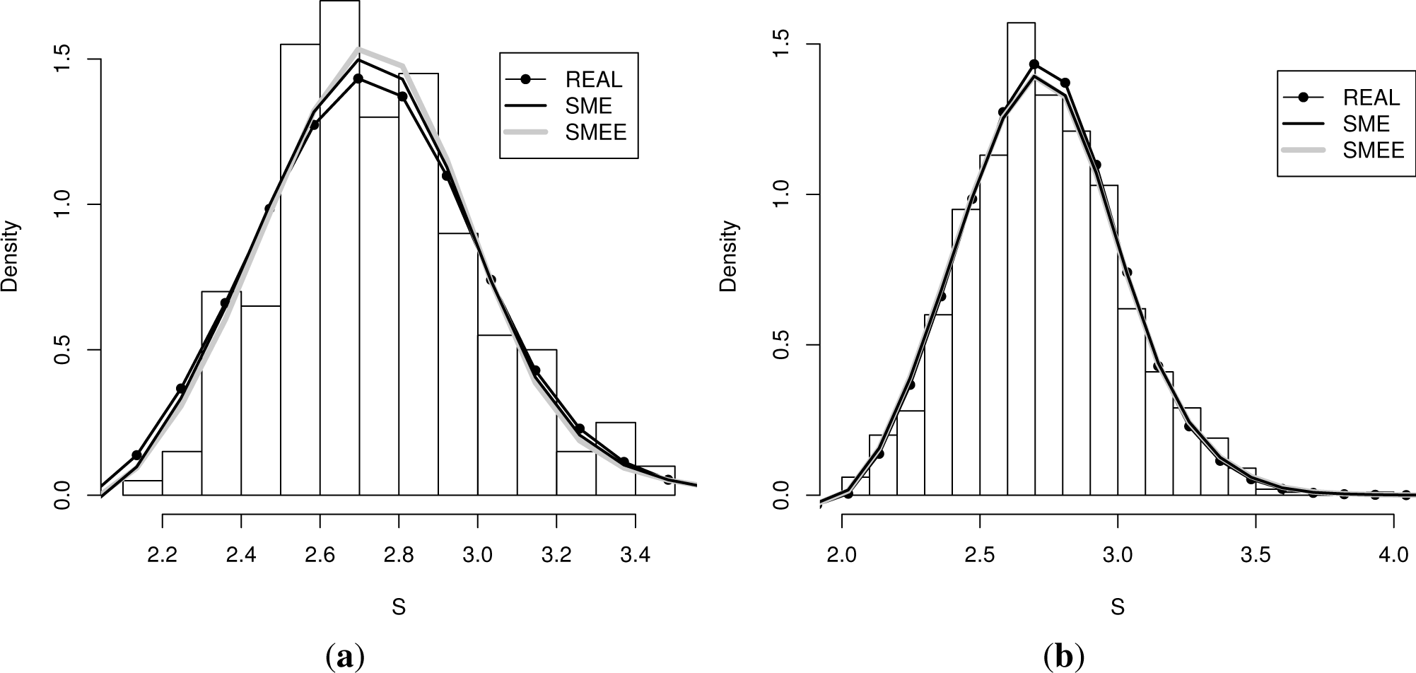
The two panels of Figure 1 display the real (true) density from which the data was sampled, the histogram that was obtained, the density reconstructed according to the SME method, as well as the density obtained according to the first extension of the SME (labeled SMEE). The left panel contains the results obtained for a sample of a size of 200, whereas the right panel the reconstruction obtained for a sample of a size of 1, 000.
Even though the moments of the density obtained with the SME method coincide with the empirical moments, the moments of the density obtained by the first reconstruction method do not need to coincide with the sample moments. They only need to fall within (or at the boundary) of the error interval, which is centered at the sample moments. In Table 3, we list the moments that those densities determine for each sample size.
Let us now run some simple quality of reconstruction tests. An experimentalist would be most interested in the comparison of the histogram (real data) to the reconstructed density. However, as we have the real density from which the data was sampled, we can perform three comparisons. We compute the actual L1 and L2 distances between the densities and those between the densities and the histograms. Actually, this is a bin-dependent computation and not a truly good measure of the quality of reconstruction, but we carry it out as a consistency test.
In Table 4, we display the results of the computations. The distances between the continuous densities are computed using standard numerical integrators and the distances between the empirical densities and the continuous densities according to:
where bk are the position of the bins, which enter as limits of integration. Note that the distances between the true density and the maxentropic reconstruction are much smaller that those between the maxentropic or trueand the histogram, and that the distance of the true and the maxentropic distances and the histogram are similar. Thus, the reconstruction methods are performing well.
Another measure of quality of reconstruction is the L1 and L2 distances between cumulative distribution functions. A simple way to compute them, which includes the histogram, as well, is given by:
where we may consider the sj to be the ordered valued of the sample without loss of generality. To distinguish them from the standard distances, MAE stands for “mean average error” and RMSE stands for “root mean square error”. The results are displayed in Table 5.
It is intuitively clear and confirmed in the results displayed in the table that the larger the size of the sample, the better the estimation results for both methods, that is, the SME and SMEE.
In Table 6, we can see details of the convergence of the method used according to the sample size. Clearly, the SMEE method involves less iterations and machine time, but involves a lower value for the gradient.
To close, let us consider Table 3 once more. We commented after Theorem 1 that when the multipliers were non-zero, the reconstructed moments are the end points of the confidence intervals. This is not borne out by the results in that table, because at a minimum, the norm of the gradient is ~ 10−4 and not exactly zero, and this tiny error explains the slight differences. Not only that, since the first method yields the boundary points of the confidence intervals as reconstructed moments, the corresponding maxentropic density is expected to differ more from the true one than that of the center of the confidence interval.
3.2. Density Reconstruction with Error Estimation
Recall that this time, we are provided with moments measured (estimated) with error and that we have prior knowledge about the range of the error about the moment. We are now interested in determining a density, the moments that it determines and an estimate of the additive measurement error.
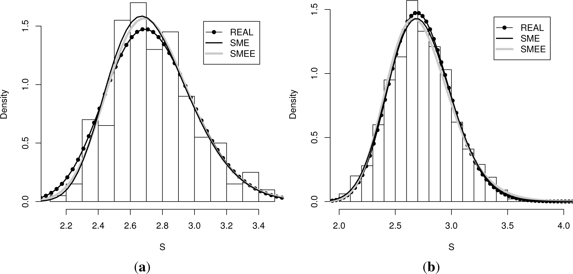
In each panel of Figure 2, we again display four plots: Along with the true (real) density and the histograms generated by sampling from it, the reconstructed maxentropic density (labeled SME) is determined by the original sample moments, and the maxentropic densities (labeled SMEE) are provided by the second procedure, for each error interval and each sample size. Visually, the SMEE densities are more close to the SME density this time.
This time, the optimal Lagrange multipliers determine both the maximum entropy distributions, as well as the weights of the endpoint of the confidence intervals for the estimation of the noise. With the multipliers, one obtains the maximum entropy density, from which the true moments can be computed as . The values obtained for each type of confidence interval and for each sample size are presented in Table 7.
Table 8 displays the estimated errors, as well as the corresponding weights of the endpoints of the error intervals. Keep in mind that the estimated error in the determination of each moment, as well as the estimated moment add up to the measured moment.
To measure the quality of the reconstructions, we again compute the L1 and L2 distances between densities, as well as the distance between distribution functions. These are displayed in Tables 9 and 10 below. Again, the distances between densities and histograms depend on the bin sizes. For a sample size of 1000, the results of the methods SME and SMEE seem to coincide better and are closer to the lognormal curve than the histogram (simulated data).
To finish, consider Table 11 in which we can show the details of the convergence of the SMEE versus the SME in the second case. The two leftmost columns compare the SMEE versus the SME for a sample of a size of 200, whereas the two rightmost columns compare the performance for a sample of a size of 1000: All things considered, it seems that the second method, that is the simultaneous determination of density and measurement errors, has a better performance.
4. Concluding Remarks
We presented and compared two possible ways of incorporating errors in the data into the usual maximum entropy formalism to determine probability densities. They correspond to two different demands about the resulting output of the method.
The first method goes as follows: For each c in the constraint space C, one solves a maximum entropy to obtain a density g*(c) having c as a constraint. Then, one varies c to find a c*, such that the entropy S(g*(c*)) of g*(c*) is maximal among all the S(g*(c)). Standard duality theory is invoked along the way to obtain the g*(c*) without having to actually determine the c*.
The second method uses both the moments and a range for the error as input data. In the first case, we simply obtain a density, whereas in the other, we obtain both a density, as well as an estimate of the error.
Recall that the only input needed for the first method is a constraint range and that we compared with SME with moments estimated from a large sample to have an idea of the performance of both procedures. We shall explore a more realistic case (small data set) elsewhere. In the example that we considered, both methods provide satisfactory results. The minimization procedure converges more slowly, and the norm of the gradient (which is a measure of the reconstruction error) is much larger in the first one of them. This is probably due to the fact that the Hessian matrix has very small eigenvalues near the minimum, making the function too flat there. Actually, both Hessians have a very small determinant, but that corresponding to the first method is about 10−20 times smaller.
This is reflected in the reconstruction error measured by the size of the gradient of the dual entropy Σ(λ) at a minimum. This is due to the flexibility of the method. Even though the L1 and L2 differences between the empirical density and the maxentropic densities are small in both procedures, the second method yields a better fit and an estimate of the measurement error, as well.
To finish, we mention that in [13], we present a detailed application of the techniques developed above to a problem of relevance in risk management.
Conflicts of Interest
The authors declare no conflict of interest.
Appendix
In the first subsection, we complete the basic modeling process missing in Section 2.2 and, then, some elementary computations useful for the minimization procedures.
A. Further Mathematical Details
To put the error estimation procedure into a model, consider the space Ω := [0, 1] × C on which we consider the obvious σ–algebra of Borel subsets, and consider the reference measure . On Ω, we define the “generalized” moments:
where ξi is the i–th coordinate of ξ. Furthermore, when P << Q0, then there exists a density f(y) and numbers pk for k = 1, …, M, such that . The maximum entropy problem can now be stated as:
Now, the procedure is standard, and the result is stated in the easy to prove, but important:
Theorem 2. Suppose that the infimum λ* of Σ(λ) given by Equation (17) is reached in the interior of the set {λ ∈ ℝM|Z(λ) < ∞}. Then, the solution to the maximum entropy problem Equation (19) is given by Equation (16).
Proof. All it takes is to differentiate (17) with respect to λi equated to zero and to read the desired conclusion.
Comment: This is a rather diluted version of the general result presented in [4] or [10], but is enough to keep us going.
In the next two subsections, we add the explicit computation of the gradient of Σ(λ) for those that use gradient-based methods for its minimization.
B. Derivative of Σ(λ) when Reconstructing with Data in a Confidence Interval
Having determined the confidence interval [ai, bi] for each i = 1, …, 8, the next step is to minimize Σ(λ). For the first case, in the case of need, here is the derivative. It invokes Equation (11):
where ki = bi if λi > 0 and ki = ai if λi < 0, and in the rare case that λi = 0, choose ki ~ U(ai, bi). Additionally, as above, .
Once the minimizer λ* has been found, the maxentropic density (in the changed variables is:
when the change of variables f*(t) = e−t g*(e−t).
C. Derivative of Σ(λ) when Reconstructing with Error Estimation
This time, the derivatives of Σ(λ) are a bit different. On the one hand:
Once the minimizing λ* has been found, the routine should be the same as above. That is, use Equation (17) to obtain the density and plot along with the result obtained in the previous section.
References
- Leipnik, R.B. On Lognormal Random Variables: I The Characteristic Function. J. Aust. Math. Soc. Series B 1991, 32, 327–347. [Google Scholar]
- Panjer, H. Operational Risk: Modeling and Analytics; John Wiley & Sons: New York, NY, USA, 2006. [Google Scholar]
- Gzyl, H.; Novi-Inverardi, P.L.; Tagliani, A. A comparison of numerical approaches to determine the severity of losses. J. Oper. Risk 2013, 8, 3–15. [Google Scholar]
- Cherny, A.; Maslov, V. On minimization and maximization of entropy functionals in various disciplines. Theory Probab. Appl 2003, 17, 447–464. [Google Scholar]
- Csiszar, I. I-divergence geometry of probability distributions and minimization problems. Ann. Probab 1975, 3, 148–158. [Google Scholar]
- Csiszar, I. Generalized I-projection and a conditional limit theorem. Ann. Probab 1984, 12, 768–793. [Google Scholar]
- Kapur, N. Maximum Entropy Models in Science and Engineering; Wiley Interscience: New York, NY, USA, 1996. [Google Scholar]
- Gzyl, H.; Velásquez, Y. Linear Inverse Problems: The Maximum Entropy Connection; World Scientific: Singapore, 2011. [Google Scholar]
- Gzyl, H.; Mayoral, S. A method for determining risk aversion functions from uncertain market prices of risk. Insur. Math. Econ 2010, 47, 84–89. [Google Scholar]
- Jaynes, E.T. Information theory and statistical physics. Phys. Rev 1957, 106, 620–630. [Google Scholar]
- Gamboa, F. Minimisation de l’information de Kullback et minimisation de l’entropie sous une contrainte quadratique. CRAS Paris, Sèrie I Math 1988, 306, 425–427. (In French). [Google Scholar]
- Borwein, J.M.; Lewis, A.S. Convex Analysis and Nonlinear Optimization; Springer Verlag: New York, NY, USA, 2000. [Google Scholar]
- Gomes, E.(Univ. Carlos III de Madrid, Getafe, Spain); Gzyl, H. (IESA, Caracas, Venezuela); Mayoral, S. (Univ. Carlos III de Madrid, Getafe, Spain). A maxentropic approach to determine operational risk losses. In preparation, 2014.


| μi | Sample size 200 | Sample size 1,000 |
|---|---|---|
| μ1 | [0.0175, 0.0177] | [0.0181, 0.0182] |
| μ2 | [0.1302, 0.1307] | [0.1318, 0.1321] |
| μ3 | [0.2559, 0.2565] | [0.2578, 0.2581] |
| μ4 | [0.3592, 0.3599] | [0.3611, 0.3614] |
| μ5 | [0.4405, 0.4412] | [0.4423, 0.4426] |
| μ6 | [0.5048, 0.5054] | [0.5065, 0.5068] |
| μ7 | [0.5565, 0.5570] | [0.5580, 0.5583] |
| μ8 | [0.5987, 0.5992] | [0.6001, 0.6004] |
| Size | Moments of S
| |||||||
|---|---|---|---|---|---|---|---|---|
| μ1 | μ2 | μ3 | μ4 | μ5 | μ6 | μ7 | μ8 | |
| 200 | 0.0176 | 0.1304 | 0.2562 | 0.3596 | 0.4409 | 0.5051 | 0.5568 | 0.5990 |
| 1,000 | 0.0181 | 0.1319 | 0.2579 | 0.3612 | 0.4424 | 0.5066 | 0.5581 | 0.6002 |
| Size | Moments of S
| |||||||
|---|---|---|---|---|---|---|---|---|
| μ1 | μ2 | μ3 | μ4 | μ5 | μ6 | μ7 | μ8 | |
| 200 | 0.0176 | 0.1302 | 0.2559 | 0.3592 | 0.4405 | 0.5048 | 0.5565 | 0.5987 |
| 1,000 | 0.0181 | 0.1319 | 0.2579 | 0.3612 | 0.4424 | 0.5066 | 0.5581 | 0.6002 |
| Approach | Histogram vs. True density | Histogram vs. Maxent | True density vs. Maxent | |||
|---|---|---|---|---|---|---|
| L1-norm | L2-norm | L1-norm | L2-norm | L1-norm | L2-norm | |
| SMEE-200 | 0.1599 | 0.1855 | 0.1504 | 0.1753 | 0.0527 | 0.0583 |
| SME-200 | 0.1599 | 0.1855 | 0.1449 | 0.1727 | 0.0668 | 0.0761 |
| SMEE-1000 | 0.1042 | 0.1077 | 0.1052 | 0.1158 | 0.0619 | 0.0577 |
| SME-1000 | 0.1042 | 0.1077 | 0.0973 | 0.1044 | 0.0307 | 0.0289 |
| Approach | Histogram vs. Real density | Histogram vs. Maxent | Real density vs. Maxent | |||
|---|---|---|---|---|---|---|
| MAE | RMSE | MAE | RMSE | MAE | RMSE | |
| SMEE-200 | 0.0158 | 0.0056 | 0.0104 | 0.0029 | 0.0106 | 0.0027 |
| SME-200 | 0.0158 | 0.0056 | 0.0089 | 0.0021 | 0.0105 | 0.0027 |
| SMEE-1000 | 0.0064 | 0.0018 | 0.0072 | 0.0024 | 0.0104 | 0.0044 |
| SME-1000 | 0.0064 | 0.0018 | 0.0043 | 0.0009 | 0.0053 | 0.0011 |
| Approach | SMEE (200) | SME (200) | SMEE (1,000) | SME (1,000) |
|---|---|---|---|---|
| time | 1.79 min | 4.33 min | 1.40 min | 3.25 min |
| iterations | 693 | 1380 | 512 | 1223 |
| min gradient | 1.06 × 10⁻⁴ | 1.86 × 10⁻⁷ | 8.81 × 10⁻⁵ | 1.72 × 10⁻⁸ |
| Size | Moments of S
| |||||||
|---|---|---|---|---|---|---|---|---|
| μ1 | μ2 | μ3 | μ4 | μ5 | μ6 | μ7 | μ8 | |
| 200 | 0.0176 | 0.1304 | 0.2561 | 0.3595 | 0.4408 | 0.5051 | 0.5567 | 0.5989 |
| 1,000 | 0.0181 | 0.1319 | 0.2579 | 0.3612 | 0.4424 | 0.5066 | 0.5581 | 0.6002 |
| SIZE | 200 | pk | 0.5143 | 0.5003 | 0.4985 | 0.4979 | 0.4975 | 0.4973 | 0.4972 | 0.4970 |
| ∈k | −1.6 × 10⁻⁶ | −1.4 × 10⁻⁷ | 8.1 × 10⁻⁷ | 1.2 × 10⁻⁶ | 1.4 × 10⁻⁶ | 1.4 × 10⁻⁶ | 1.5 × 10⁻⁶ | 1.4 × 10⁻⁶ | ||
| 1000 | pk | 0.5016 | 0.5071 | 0.5036 | 0.5008 | 0.4987 | 0.4972 | 0.4960 | 0.4951 | |
| ∈k | −1 × 10⁻⁷ | −1.5 × 10⁻⁶ | −1 × 10⁻⁶ | −2.4 × 10⁻⁷ | 3.6 × 10⁻⁷ | 7.8 × 10⁻⁷ | 1 × 10⁻⁶ | 1.2 × 10⁻⁶ |
| Approach | Histogram vs. Real density | Histogram vs. Maxent | Real density vs. Maxent | |||
|---|---|---|---|---|---|---|
| L1-norm | L2-norm | L1-norm | L2-norm | L1-norm | L2-norm | |
| SMEE-200 | 0.1599 | 0.1855 | 0.1474 | 0.1748 | 0.0761 | 0.0804 |
| SME-200 | 0.1599 | 0.1855 | 0.1449 | 0.1727 | 0.0668 | 0.0761 |
| SMEE-1000 | 0.1042 | 0.1077 | 0.0977 | 0.1051 | 0.0325 | 0.0301 |
| SME-1000 | 0.1042 | 0.1077 | 0.0973 | 0.1044 | 0.0307 | 0.0289 |
| Approach | Histogram vs. Real density | Histogram vs. Maxent | Real density vs. Maxent | |||
|---|---|---|---|---|---|---|
| MAE | RMSE | MAE | RMSE | MAE | RMSE | |
| SMEE-200 | 0.0158 | 0.0056 | 0.0094 | 0.0023 | 0.0134 | 0.0037 |
| SME-200 | 0.0158 | 0.0056 | 0.0089 | 0.0021 | 0.0105 | 0.0027 |
| SMEE-1000 | 0.0064 | 0.0018 | 0.0043 | 0.0009 | 0.0057 | 0.0013 |
| SME-1000 | 0.0064 | 0.0018 | 0.0043 | 0.0009 | 0.0053 | 0.0011 |
| Approach | SMEE (200) | SME (200) | SMEE (1000) | SME (1000) |
|---|---|---|---|---|
| time | 37.48 s | 4.33 min | 18.95 s | 3.25 min |
| iterations | 220 | 1380 | 112 | 1223 |
| min gradient | 1.07 × 10⁻¹⁰ | 1.86 × 10⁻⁷ | 5.82 × 10⁻¹⁰ | 1.72 × 10⁻⁸ |
© 2014 by the authors; licensee MDPI, Basel, Switzerland This article is an open access article distributed under the terms and conditions of the Creative Commons Attribution license (http://creativecommons.org/licenses/by/3.0/).
Share and Cite
Gomes-Gonçalves, E.; Gzyl, H.; Mayoral, S. Density Reconstructions with Errors in the Data. Entropy 2014, 16, 3257-3272. https://doi.org/10.3390/e16063257
Gomes-Gonçalves E, Gzyl H, Mayoral S. Density Reconstructions with Errors in the Data. Entropy. 2014; 16(6):3257-3272. https://doi.org/10.3390/e16063257
Chicago/Turabian StyleGomes-Gonçalves, Erika, Henryk Gzyl, and Silvia Mayoral. 2014. "Density Reconstructions with Errors in the Data" Entropy 16, no. 6: 3257-3272. https://doi.org/10.3390/e16063257
APA StyleGomes-Gonçalves, E., Gzyl, H., & Mayoral, S. (2014). Density Reconstructions with Errors in the Data. Entropy, 16(6), 3257-3272. https://doi.org/10.3390/e16063257