Equivalent Temperature-Enthalpy Diagram for the Study of Ejector Refrigeration Systems

Abstract
: The Carnot factor versus enthalpy variation (heat) diagram has been used extensively for the second law analysis of heat transfer processes. With enthalpy variation (heat) as the abscissa and the Carnot factor as the ordinate the area between the curves representing the heat exchanging media on this diagram illustrates the exergy losses due to the transfer. It is also possible to draw the paths of working fluids in steady-state, steady-flow thermodynamic cycles on this diagram using the definition of “the equivalent temperature” as the ratio between the variations of enthalpy and entropy in an analyzed process. Despite the usefulness of this approach two important shortcomings should be emphasized. First, the approach is not applicable for the processes of expansion and compression particularly for the isenthalpic processes taking place in expansion valves. Second, from the point of view of rigorous thermodynamics, the proposed ratio gives the temperature dimension for the isobaric processes only. The present paper proposes to overcome these shortcomings by replacing the actual processes of expansion and compression by combinations of two thermodynamic paths: isentropic and isobaric. As a result the actual (not ideal) refrigeration and power cycles can be presented on equivalent temperature versus enthalpy variation diagrams. All the exergy losses, taking place in different equipments like pumps, turbines, compressors, expansion valves, condensers and evaporators are then clearly visualized. Moreover the exergies consumed and produced in each component of these cycles are also presented. The latter give the opportunity to also analyze the exergy efficiencies of the components. The proposed diagram is finally applied for the second law analysis of an ejector based refrigeration system.1. Introduction
Utilisation of ejector refrigeration cycles powered by waste heat or solar energy is an important alternative to absorption machines such as LiBr-H2O and H2O-NH3 [1,2]. Construction, installation and maintenance of such systems are relatively inexpensive compared to that of absorption machines. The temperature-entropy diagram is usually used to describe the behaviour of the ejector refrigeration cycles [3,4], however this diagram does not allow one to evaluate the irreversibilities, their distribution within the cycle, as well as the exergy efficiency of its components. The Carnot factor-enthalpy diagram has been used extensively for the second law analysis of heat transfer processes [5,6]. With enthalpy variation (heat) as the abscissa and the Carnot factor as the ordinate the area between the special curves, representing the heat exchanging media on this diagram, illustrates the exergy losses due to the transfer. The diagram has been applied for the thermodynamic analysis of individual heat exchangers [5] as well as for heat exchanger networks [6]. The introduction of the “equivalent temperature” allowed the sorption refrigeration cycles to be presented on this diagram [7]. Meanwhile the difficulties to present expansion and compression processes on the Carnot factor-enthalpy diagram limit its application to the ejector refrigeration cycles. The main objective of the present paper is to overcome this limitation by replacing the actual processes of expansion and compression by combinations of two thermodynamic paths: isobaric and isentropic. To explain this new approach the classical power cycle (Organic Rankine Cycle, ORC) and mechanical refrigeration cycle will be firstly presented on the Carnot factor-enthalpy diagram. Afterwards, following the work of Arbel et al. [8], the ejector refrigeration cycle will be presented as a superposition of the power and refrigeration cycles. It will allow presenting the ejector refrigeration cycle on the diagram. As a result the exergy losses as well as the exergies consumed and produced in each element of the ejector refrigeration cycle will be quantified and visualized on the diagram.
2. Equivalent Temperature
According to Prigogine [9] two thermodynamic processes are equivalent if the entropy production for each of them is the same. Following this definition, Bejan et al. [10] introduced the notion of “the equivalent temperature” as:
Given that the term (Tds) can be expressed as a function of enthalpy variation (dh):
Equation (1) can be rewritten as:
Neveu and Mazet [7] defined the equivalent temperature (Teq) simply by the ratio between the variations of enthalpy and entropy in an analyzed process:
The later relation gave the opportunity to present a refrigeration cycle on the Carnot factor-enthalpy diagram. The Carnot factor was associated with (Teq) by the following expression:
The comparison between Equations (3) and (4) shows that from the point of view of rigorous thermodynamics, the ratio (4) gives the correct equivalent temperature for isobaric processes only. This fact does not allow the application of the Carnot factor-enthalpy diagram [7] to compression and expansion processes. Moreover according to the definition (4) the equivalent temperature of a throttling process (dh = 0) is zero, as a result the exergy losses due to this process cannot be presented on such a diagram. Yet the application of ratio (4) is attractive because of its simplicity that already allowed the diagrammatic analysis of sorption refrigeration systems [5,6].
To keep the definition (4) for the analysis of ejector refrigeration cycles it is proposed to replace the adiabatic processes of expansion and compression by combinations of two thermodynamic paths: isentropic and isobaric. The value of Teq for an isentropic process equals to (∞) which means that, according to (5), Θeq = 1. For an isobaric process the values of Teq and Θeq may be calculated by using the formulas (4) and (5) respectively. The next section will illustrate the application of this new approach to an ORC cycle.
3. Organic Rankine Cycle
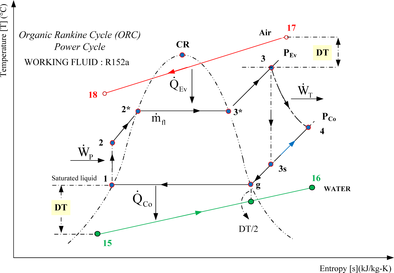
The T-s diagram of the analyzed ORC is illustrated in Figure 1. The cycle was studied by Khennich and Galanis [11]. The working fluid is R152a. The cycle is used to recover the waste heat contained in a low temperature airstream rejected by an industrial process. This flow enters the evaporator at the temperature T17 = 115 °C, the mass flow rate is . The temperature of the cooling water at the condenser entry is T15 = 10 °C and the mass flow rate is . The working fluid receives heat at a relatively high pressure in the evaporator, is then expanded in a turbine, thereby producing useful work, and rejects heat at a low pressure in the condenser. It is then pumped to the evaporator. The isentropic efficiency of the pump is taken as ηp = 1. The isentropic efficiency of the turbine is equal to ηT = 0.8. The temperature difference between the external fluid inlet and the working fluid exit is taken as DT = 5 °C. The same DT is assumed for evaporator and condenser. The dimensionless value of the net power of the cycle α is obtained by dividing by the following reference power: . The chosen value of α (=0.08) corresponds to a mass flow rate of working fluid 4.177 kg/s. Finally, the evaporation pressure is considered equal to PEv = 1000 kPa. (PCo < PEv < PSat(T3)).
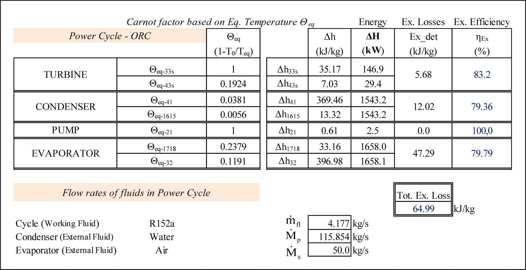
The adiabatic expansion path 3–4 is replaced by the combination of the isentropic path 3–3s and the isobaric 3s–4. The mathematical model of the cycle was solved by using the EES [12] code which includes the thermodynamic properties of R152a. The computational results, including Θeq, the corresponding enthalpy variations as well as the exergy losses and exergy efficiencies of each component of the cycle are presented in Figure 2.
The Carnot factors corresponding to the isentropic expansion 3–3s and isentropic compression 1–2 equal 1, because the equivalent temperatures are infinitely large. The largest exergy losses take place at the evaporator, 197.53 kW (47.29 kJ/kg) and represent 72.77% of the total exergy destroyed 271.42 kW (64.99 kJ/kg) in the ORC system. However the exergy efficiency of the evaporator is relatively high, almost 80% which means that the further reduction of exergy losses may require an economically prohibitive increase in heat transfer area. The Θeq vs. ΔH results from Figure 2 are used to build the corresponding diagram presented in Figure 3.
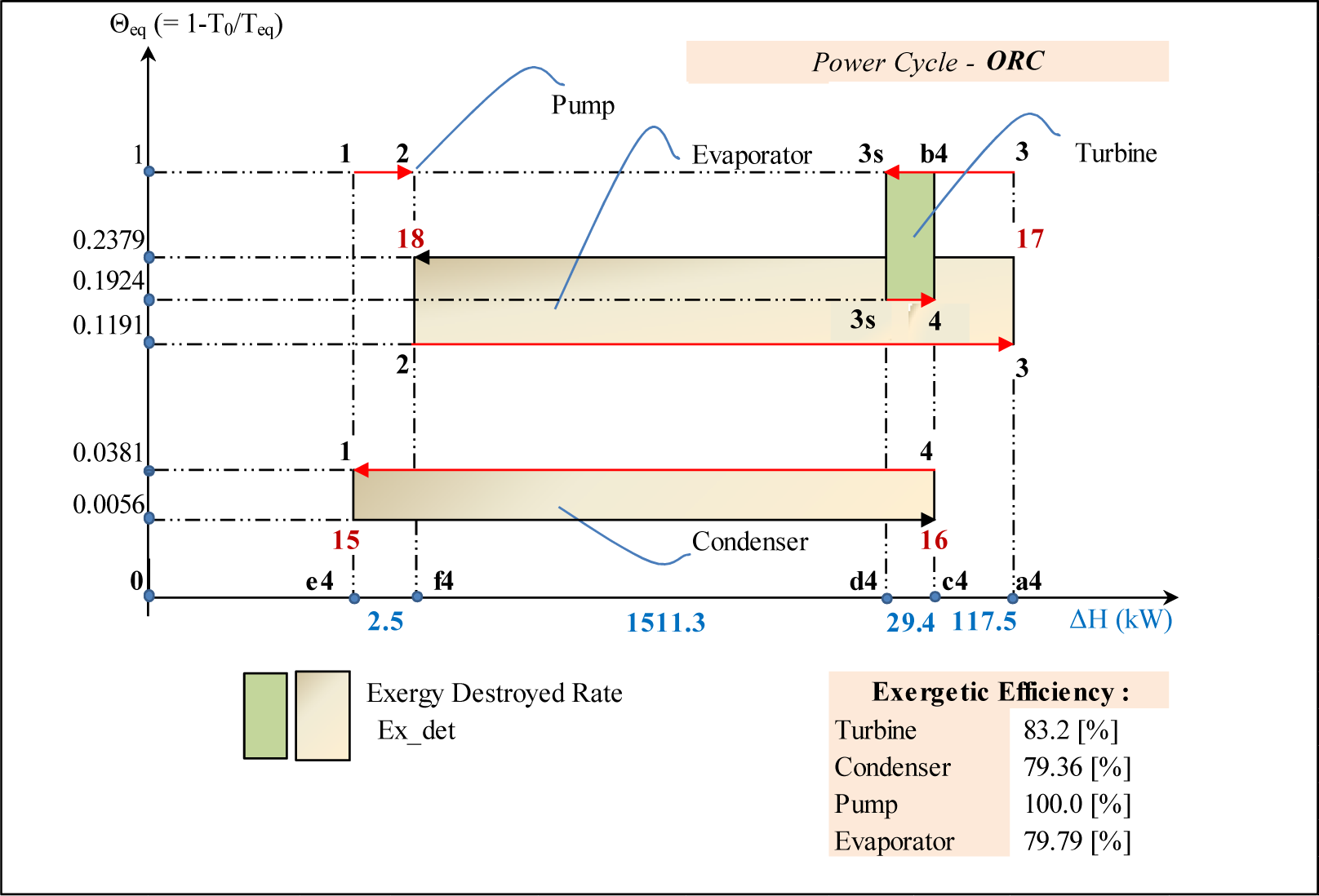
Although Figure 3 is not to scale, the information shown represents exactly the quantitative results of the analysis. For example, the exergy destruction in the turbine, in (kJ/kg), illustrated by the green rectangle in Figure 3 is equal to:
This result is identical to the corresponding value shown in Figure 2. The way to draw this diagram is to follow a particle of working fluid all along the cycle. It should be noted that the same point on T-s diagram is characterized by different equivalent temperatures depending on the process with which it is associated; it is therefore represented by multiple points on the same vertical line in the Θeq-ΔH diagram. For example point 3 on Figure 1 is the final state for the evaporation process 3–2 (Θeq = 0.1191) and the initial one for the expansion path 3–3s (Θeq = 1); as a result it is represented as two points on the same vertical line on Figure 3. Thus all the processes on the Θeq-ΔH diagram are presented by horizontal lines. The direction of the arrow corresponds to the direction of the working flow. The isentropic expansion is presented by the line 3–3s at Θeq = 1; the frictional (adiabatic) reheat of the turbine by line 3s–4 at Θeq = 0.1924; the condensation by 4–1 at Θeq = 0.0381; the isentropic pumping by 1–2 at Θeq = 1 and the evaporation by 3–2 at Θeq = 0.1191. The external fluids, hot gas and cooling water are presented by lines 17–18 and 16–15 respectively.
The closure of the energy balance of the cycle can be easily verified on this diagram. Indeed:
The results of the exergy analysis presented in Figure 2 are visually illustrated on the diagram of Figure 3. The exergy losses in each component of the ORC cycle are shown as surfaces and are the product of the enthalpy change ΔH in (kW) and the variation of the equivalent Carnot factor. The environmental temperature T0 = 283 K (10 °C) is taken equal to the water temperature in the condenser. Moreover the diagram allows visualizing the exergy produced and expended in each element. Their ratio gives the value of exergy efficiency, Brodyansky et al. [13]. For example the area a4–3–b4–4–3s–d4 corresponds to the exergy produced by the turbine. It is composed of two useful effects: the shaft work from the turbine (the area a4–3–b4–c4) and the exergy of the frictional reheat (the area c4–4–3s–d4). The expended exergy is presented by the area a4–3–3s–d4 and corresponds to the exergy produced in the ideal isentropic turbine. The exergies produced in the evaporator and condenser are a4–3–2–f4 and c4–16–15–e4 respectively; the expanded exergies are a4–17–18–f4 and c4–4–1–e4 respectively.
4. Mechanical Refrigeration Cycle
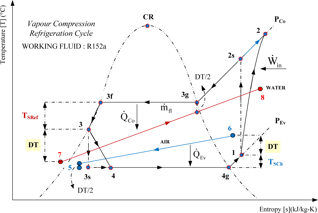
The refrigeration mechanical vapor compression cycle is shown in Figure 4. The working fluid is R152a, the same as for the ORC. It enters the compressor at T1 = −10 °C, (T1 = T4g + 6 °C) in the form of superheated steam (6 °C overheating at the outlet of evaporator). The isentropic compressor efficiency is ηComp = 0.85. At the entrance of the condenser the fluid is in the form of superheated steam. It flows through the condenser by giving up heat to the external fluid (water). At the inlet of the expansion valve it is in the form of subcooled liquid (6 °C subcooling at the outlet of the condenser) T3 = 20 °C, (T3 = T3f − 6 °C). It undergoes a pressure drop in the valve reaching the evaporation pressure at its outlet. Emerging from the valve, the fluid enters the evaporator as a liquid-vapor mixture. As it passes through the evaporator, it absorbs heat from the air, which enters at a temperature of 0 °C. The fluid finally leaves the evaporator in the form of superheated steam to be admitted into the compressor. The inlet temperature of the external fluid (water) in the condenser is 10 °C; a mass flow rate = 4 kg/s. The temperature difference between the refrigerant and the external fluid in the condenser and evaporator is DT = 10 °C. Refrigerant mass flow rate is = 0.15 kg/s. The flow regime is permanent and variations of the kinetic and potential energy are neglected. The throttling process 3–4 is replaced by the combination of the isentropic expansion path 3–3s and the isobaric-isothermal path 4–3s.
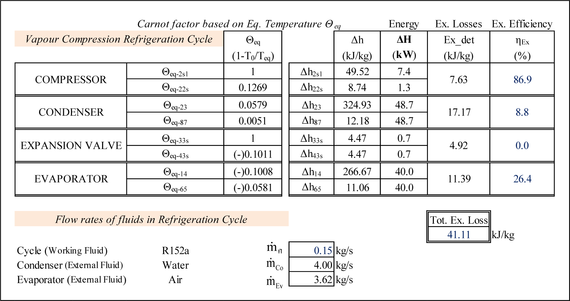
Similar to the ORC cycle the computational results, including Θeq, the corresponding enthalpy variations as well as the exergy losses and exergy efficiencies of each component of the refrigeration cycle are presented in Figure 5.
Unlike the results for the ORC, Figure 5 illustrates that the biggest exergy losses take place in the heat exchangers of the refrigerating cycle. In the condenser, this translates into 41.77% of the total exergy destroyed in this cycle. The evaporator follows with 27.71% of the total exergy losses of the cycle. All exergy expended in the valve is destroyed by the irreversibility, thus its exergy efficiency is nil.
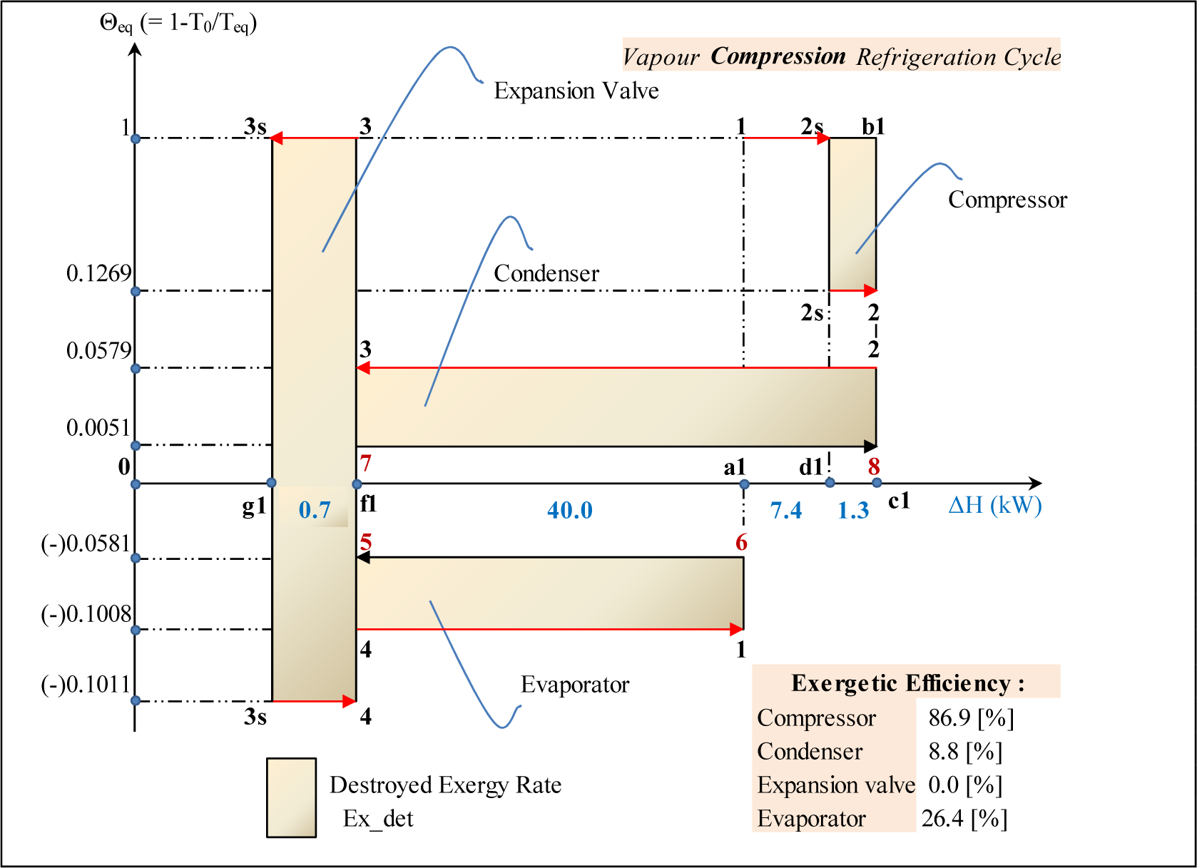
The Θeq-ΔH diagram of the cycle is presented on Figure 6. The isentropic compression is presented by the line 1–2s at Θeq = 1; the frictional (adiabatic) reheat of the compressor by line 2s–2 at Θeq = 0.1269; the condensation by 2–3 at Θeq = 0.0579; the isentropic expansion path by 3–3s at Θeq = 1; the isobaric-isothermal path by 3s–4 at Θeq = −0.1011 and the evaporation by 4–1 at Θeq = −0.1008. The external fluids, air and cooling water are presented by lines 6–5 and 7–8 respectively. Again the closure of the energy balance of the cycle can be easily verified on this diagram:
The diagram reveals the nature of exergy losses in the throttling valve. Indeed they are presented as a summation of two areas: the first (f1–3–3s–g1–f1) corresponds to the lost potential to produce shaft work due to the expansion, the second (f1–g1–3s–4–f1) illustrates the exergy lost due to the reduced refrigeration capacity in the evaporator.
The exergy produced by the compressor is presented by the area a1–1–2s–2s–2–c1. It is the sum of two components: the minimum shaft work to drive the isentropic compression (the area a1–1–2s–d1) and the exergy of the frictional reheat (the area d1–2s–2–c1). The expended exergy is presented by the area a1–1–b1–c1 and corresponds to the shaft work required to drive the real adiabatic compressor. The interpretation of the areas corresponding to exergies produced and expanded in heat exchangers are similar to the ORC case.
5. Ejector Refrigeration System
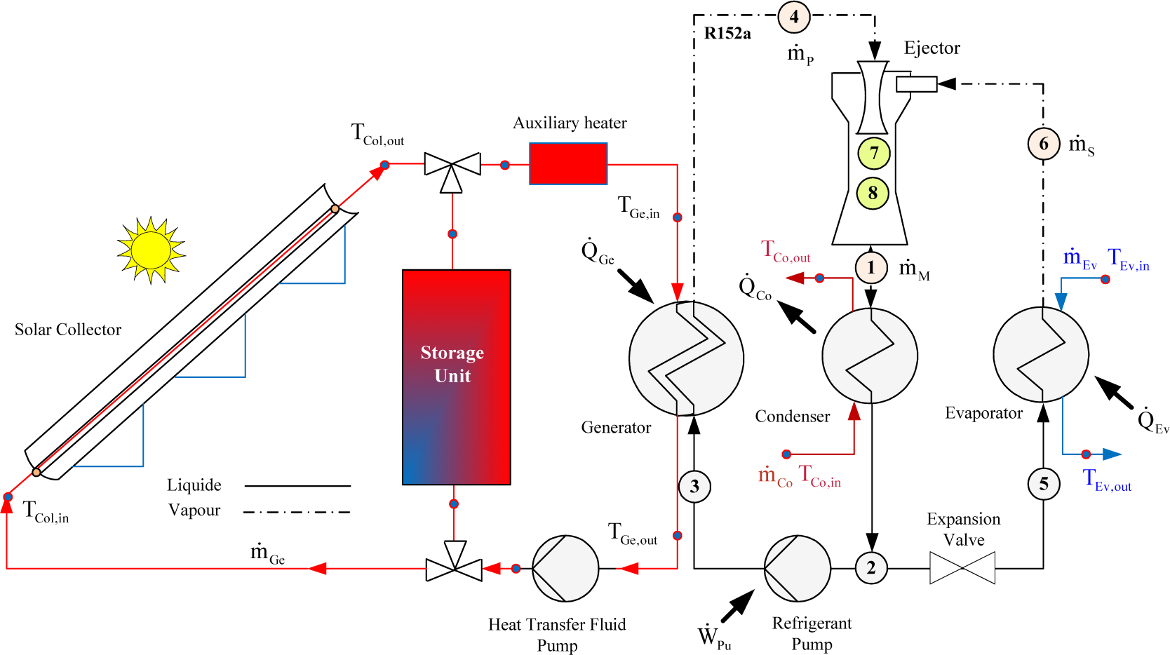
The ejector refrigeration cycle driven by solar energy is illustrated in Figure 7. The cycle has been studied under the condition of minimizing the total thermal conductance (UAt) of the three heat exchangers (generator, condenser and evaporator). The corresponding optimum value of pressure at the generator is PGe,opt = 3000 kPa resulting in a minimum total thermal conductance of UAt,min = 10.65 kW/K. The refrigerant used is R152a. External fluids at the generator, condenser and evaporator are respectively: XcelTherm500, water and the anti-freezing fluid MEG 45% (monoethylene glycol 45%) as a coolant at low temperature. The refrigeration capacity has been set to a value of 10 kW. The minimum temperature difference in the heat exchangers is DT = 5 °C. The temperature of the fluid entering the generator is TGe,in = 105 °C, the temperature of the cooling water entering the condenser is TCo,in = 10 °C and the temperature of the refrigeration fluid entering the evaporator is TEv,in = 0 °C.
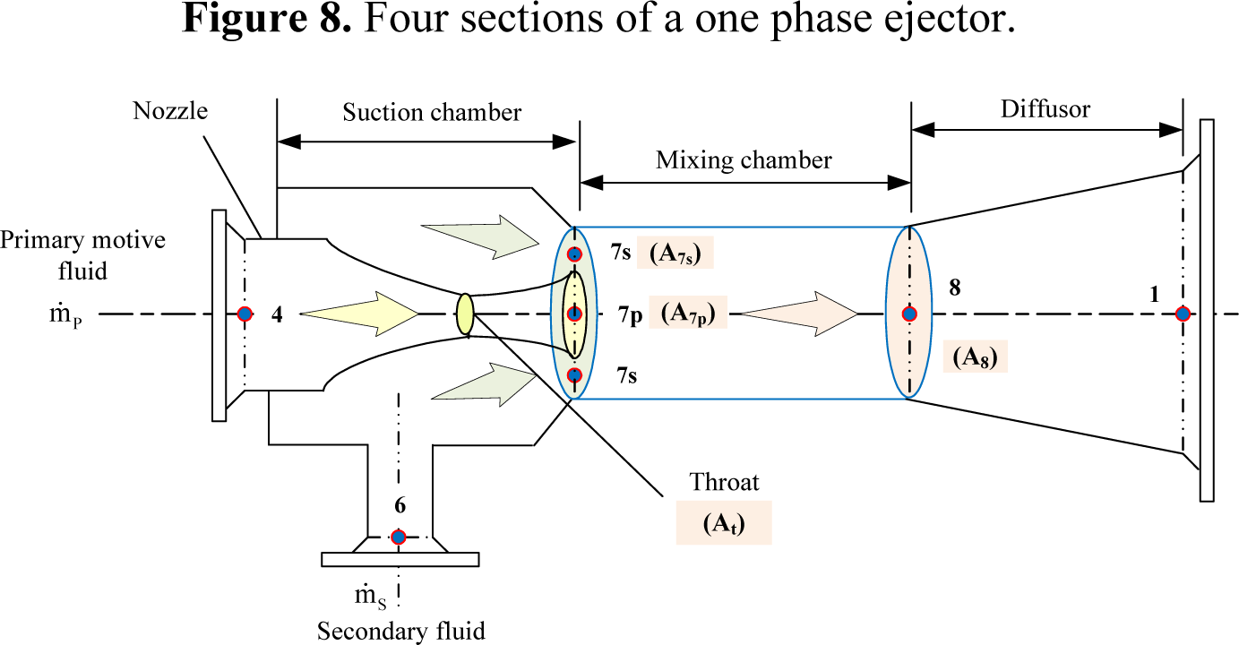
Figure 8 illustrates the four sections of an ejector: nozzle, suction chamber, mixing chamber and diffuser. The computational model used in the present study is based on the hypothesis of constant area of mixing chamber Dahmani et al. [3].
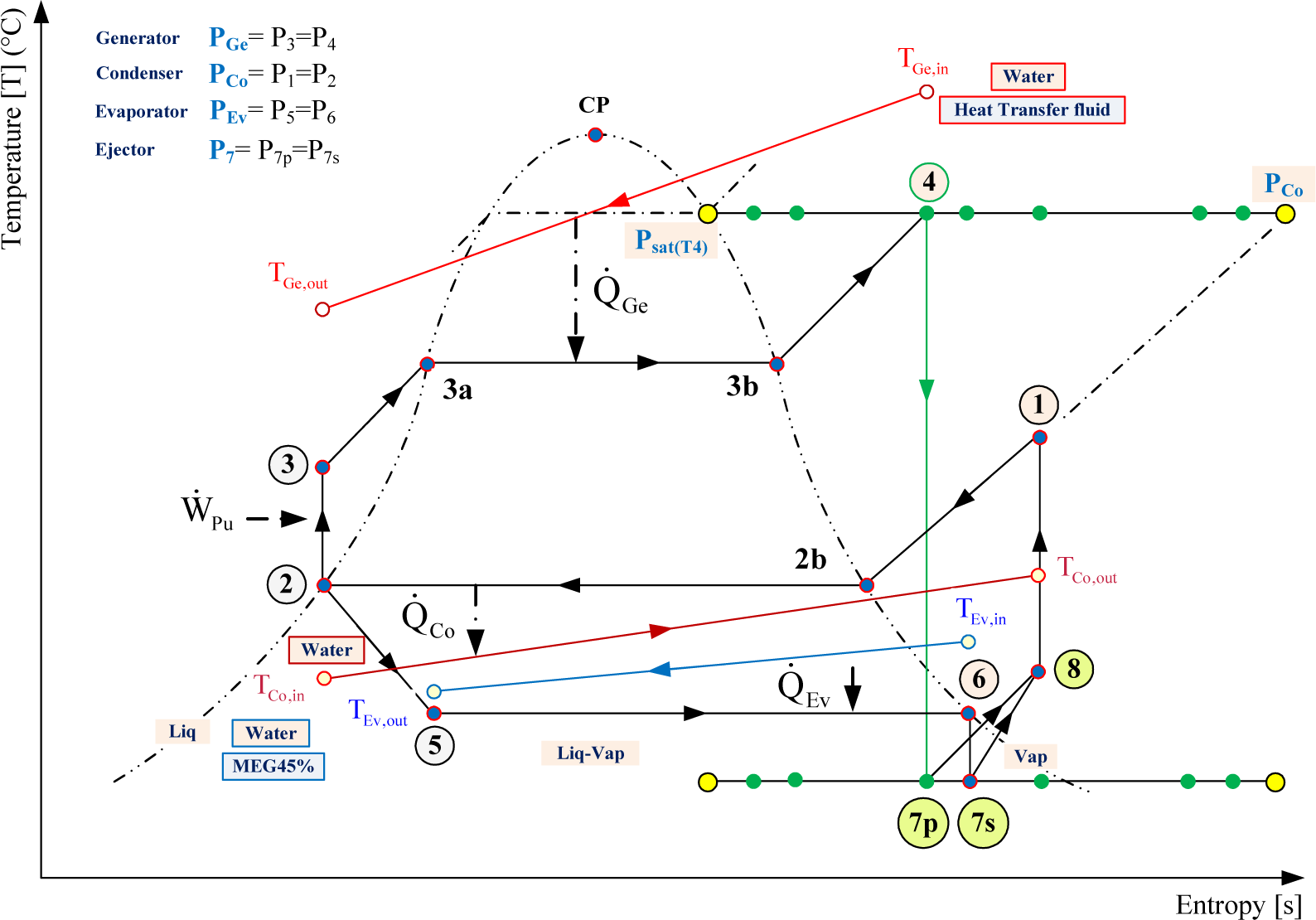
Figure 9 shows a temperature-entropy diagram of the processes taking place in the system presented on Figure 7 and the ejector on Figure 8. According to Dahmani et al. [3] the high pressure vapor at 4 expands isentropically in a converging–diverging nozzle to a very low pressure 7p and aspirates the saturated vapor from 6. The later expands to a pressure 7s, the same as at 7p. These two low pressure streams mix irreversibly in a constant area chamber emerging at state 8. Finally this mixture is decelerated isentropically to state 1 in a diffuser.
The states of the refrigerant at all points of Figures 7 and 8 are calculated according to the procedure described by Dahmani et al. [3] using the following inputs: R152a, , (XcelTherm500, TGe,in = 105 °C), (Water, TCo,in = 10 °C), (MEG45%, TEv,in = 0 °C), DT = 5 °C, . This procedure considers that the acceleration of the primary and secondary fluids from 4 to 7p and from 6 to 7s respectively as well as the deceleration of the mixture from 8 to 1 are reversible and adiabatic (see Figure 9). On the other hand the mixing process which occurs between planes 7 and 8 is adiabatic but irreversible resulting in a significant entropy increase (see Figure 9) and exergy destruction. We thus obtain the values of the pressure, the temperature, the entropy, etc. at all the states shown in Figures 7 and 8. In particular we obtain the entropy increase associated with the irreversible mixing process which takes place between planes 7 (where the two streams have the same pressure, P7p = P7s = 128.4 kPa, but different velocities and entropies) and 8 (where the flow is fully mixed). Thus, s4 = s7p = 2.050 kJ/(kg·K), s6 = s7s = 2.131 kJ/(kg·K) and s8 = s1 = 2.160 kJ/(kg·K). We are also able to calculate the rate of exergy destruction associated with this irreversible mixing process. It should be noted that the rate of exergy destruction for the entire ejector is the same as that of the mixing process since the expansion of the two fluids and the deceleration of the mixture in the diffuser are considered to be reversible.
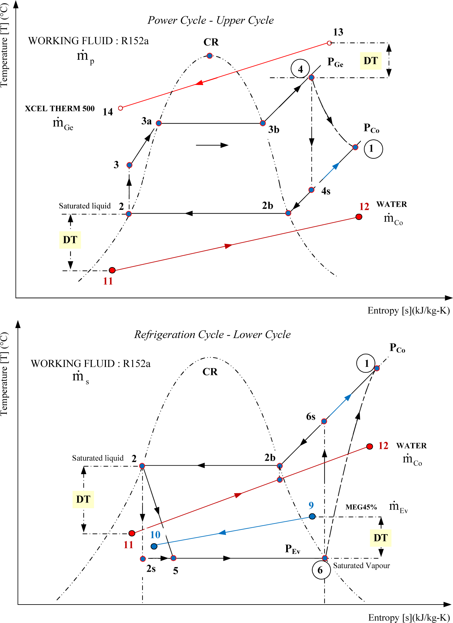
Following the work of Arbel et al. [8], the ejector refrigeration cycle can be presented as a superposition of the power (2–3–4–7p–8–1) and refrigeration (2–5–6–7s–8–1) sub-cycles. By using the isentropic and isobaric paths between points (4, 1) and (6, 1) these two sub-cycles are presented separately on Figure 10. The power cycle is named Upper Cycle (UC) and refrigeration cycle Lower Cycle (LC).
The power sub-cycle or Upper Cycle (UC) shown in Figure 10 is drawn using the intensive properties (temperature, pressure, specific entropy) of states 1, 2, 3 and 4 calculated by the Dahmani et al. [3] model for the cycle of Figure 9. It shows that the primary or motive fluid enters the ejector at state 4 and exits at state 1 with a considerable entropy increase caused by the irreversible phenomena taking place in the ejector. Similarly, the refrigeration sub-cycle or Lower Cycle (LC) of Figure 10 drawn with the intensive properties of states 1, 2, 5 and 6 (calculated by the model for the cycle of Figure 9) shows the corresponding entropy increase for the secondary or entrained fluid which enters the ejector at state 6 and exits at state 1. It should be noted that the two sub-cycles have the same intensive properties at states 1 and 2. The mass flow rates for the upper and lower sub-cycles are equal to primary and secondary mass flow rates of the ejector respectively.
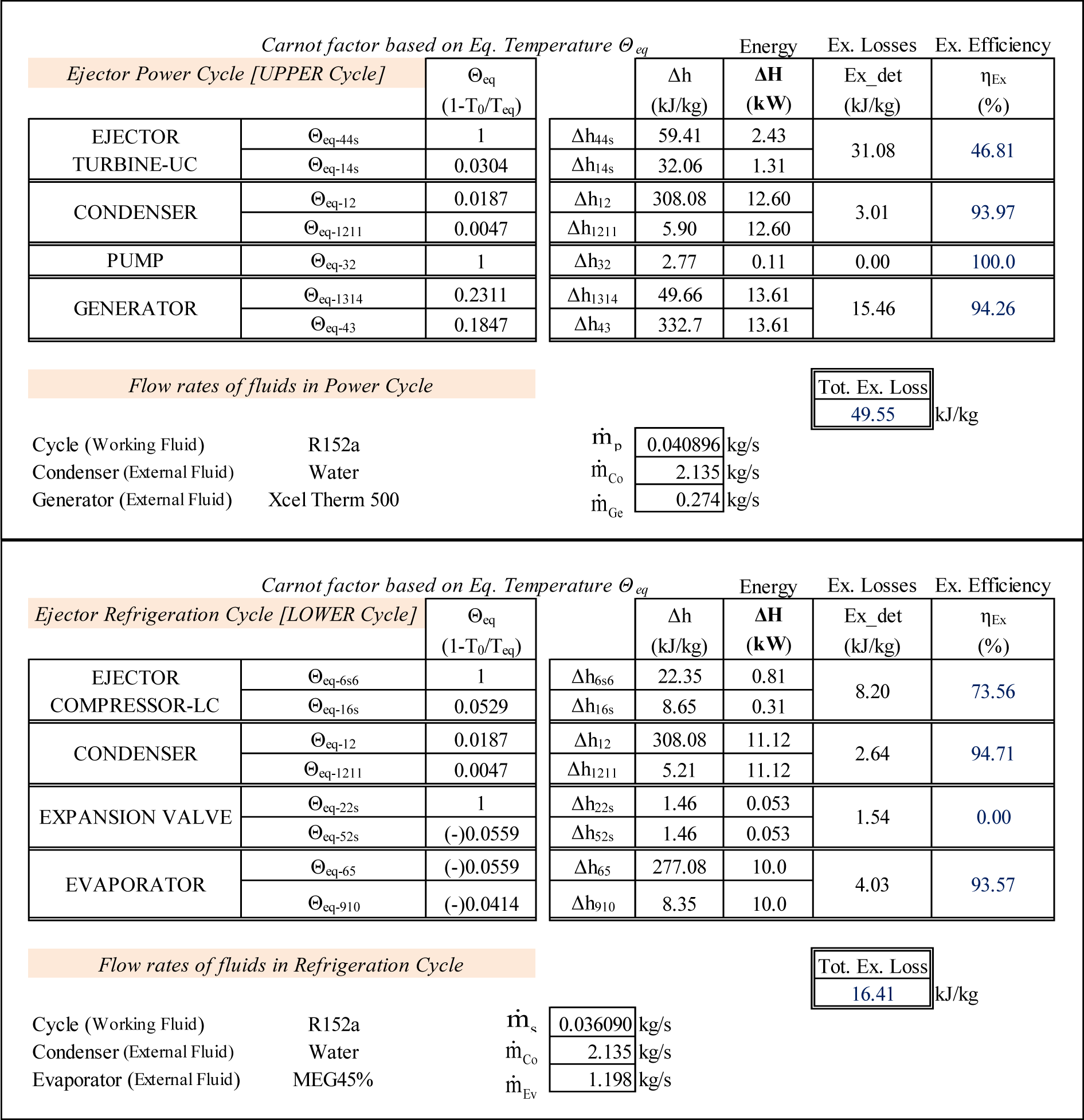
The computational results, including Θeq, the corresponding enthalpy variations as well as the exergy losses and exergy efficiencies of each component of the two sub-cycles are presented in Figure 11.
The irreversibility of the phenomena occurring in the entire ejector (see Figure 9) is equal to the sum of those occurring in the turbine of the Upper Cycle and the compressor of the Lower Cycle between states 4–1 and 6–1 respectively.
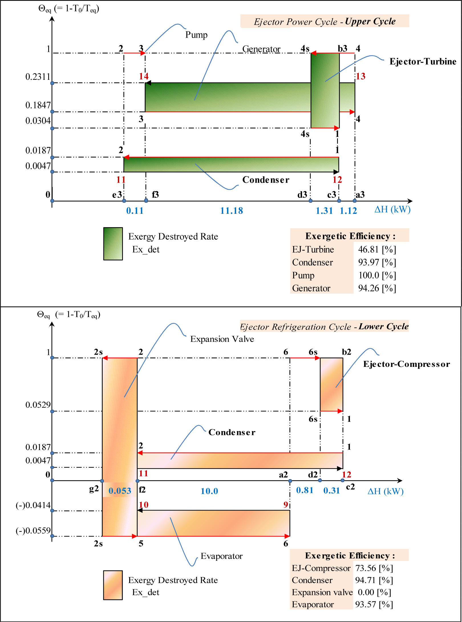
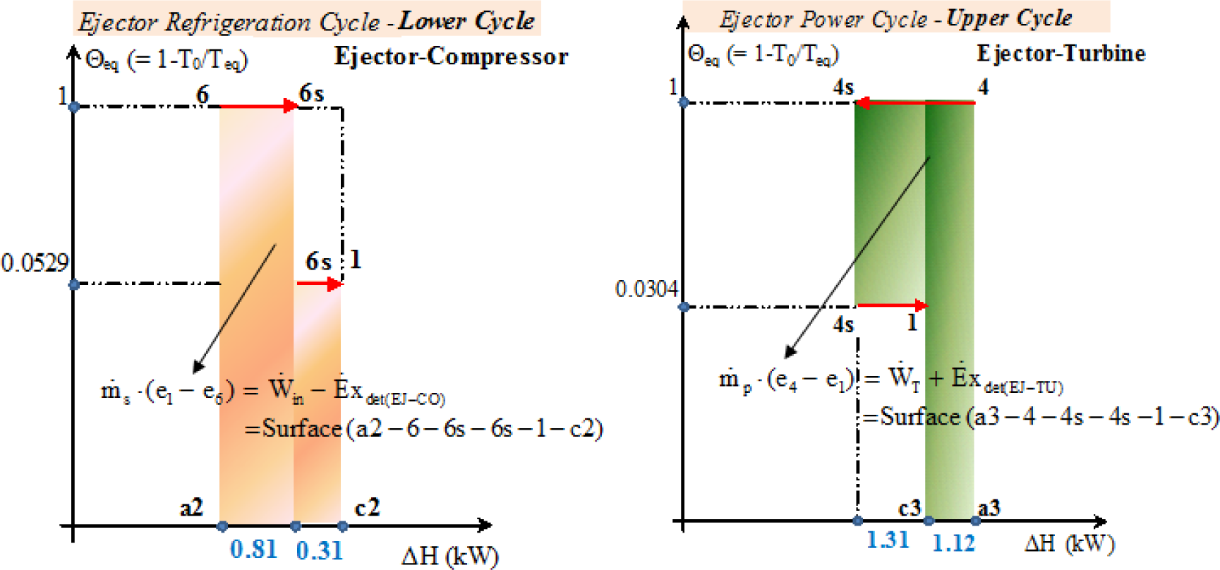
The Θeq-ΔH diagrams of the two sub-cycles are presented on Figure 12. For the UC the isentropic expansion of the motive stream is presented by the line 4–4s at Θeq = 1; the frictional (adiabatic) reheat by line 4s–1 at Θeq = 0.0304. For the LC the isentropic compression is presented by the line 6–6s at Θeq = 1 whereas the frictional (adiabatic) reheat of the compressor is by line 6s–1 at Θeq = 0.0529. The presentations of the processes in heat transfer equipment are similar to the diagrams on Figures 3 and 6.
Again, even though Figure 12 is not to scale, the information shown represents exactly the quantitative results of the analysis. For example, the exergy destruction, in (kJ/kg), in the expansion valve is equal to:
The difference between this result and the corresponding value in Figure 11 is (0.01) kJ/kg (i.e., less than 1%) and is due to rounding of errors.
Given that the ejector and the condenser are the pieces of equipment which connect the two sub-cycles, UC and LC, the exergy losses in (kW) calculated separately in these two components will therefore be added.
Figure 13 is the zooming of the useful exergy produced (the left diagram) and the exergy expended (the right diagram) in the ejector taken from Figure 12.
Based on Figure 13 the exergy efficiency in (%) is defined as:
This value is relatively low and emphasises the necessity to improve the thermodynamic efficiency of the ejector in the ejector refrigeration cycle.
6. Conclusions
A special Carnot factor-enthalpy diagram based on “the equivalent temperature” has been proposed to analyse the exergy performance of ejector refrigeration cycles.
The exergy losses as well as the exergies consumed and produced in each component of the ejector refrigeration cycle are qualitatively visualized on the diagram.
The diagram pinpoints the low exergy efficiency of the ejector inside the ejector refrigeration cycle.

| A | Area | m2 |
| DT | Temperature difference between working fluid and external fluid | °C |
| e | Specific flow exergy | kJ/kg |
| Eq. Temp. | Equivalent Temperature | |
| Exergy destruction rate | kW | |
| Exergy rate (Inlet) | kW | |
| Exergy rate (Outlet) | kW | |
| GWP | Global warming potential, relative to CO2 | |
| h | Specific enthalpy | kJ/kg |
| Mass flowrate of working fluid | kg/s | |
| Mass flowrate of sink and source | kg/s | |
| ODP | Ozone depletion potential, relative to R11 | |
| ORC | Organic Rankine Cycle | |
| P | Pressure | kPa, MPa |
| Heat transfer rate | kW | |
| s | Specific entropy | kJ/kg-K |
| T, Temp, t | Temperature, (t) is in K | °C, K |
| UA | Thermal conductance | kW/K |
| Power input or output | kW | |
| ΔH | Enthalpy variation rate: | kW |
| Greek symbols | ||
| α | Non-dimensional net power output | |
| η | Efficiency | |
| ∆ | Difference | |
| Θ | Carnot Factor, Θ = (1 − T0/T) | |
| Subscripts | ||
| 0 | Dead state | |
| 1, 2…3*… | States of thermodynamic cycle | |
| Co | Condenser, condensation | |
| CO, comp | Compressor, compression | |
| CR | Critical | |
| det | Destruction, destroyed | |
| Ej | Ejector | |
| Ev | Evaporator, evaporation | |
| Eq, eq | Equivalent | |
| ex | exergetic | |
| fl | Fluid | |
| g | Saturated vapor | |
| Ge | Generator | |
| in | Inlet, Input | |
| is | Isentropic | |
| LC | Lower Cycle | |
| min | Minimal, minimum | |
| opt | Optimal | |
| out | Outlet, Output | |
| p | Sink, primary | |
| P | Pump | |
| ref | reference | |
| s | Source, secondary | |
| SCH | Superheating | |
| SRef | Subcooling | |
| t | Total | |
| T, TU | Turbine | |
| UC | Upper Cycle | |
| VC | Control volume | |
| w | Specific work (inlet or outlet) | |
Acknowledgments
The authors would like to thank CanmetENERGY research center of Natural Resources Canada for its support of this study.
Author Contributions
Mohammed Khennich: Principal Investigator; Mikhail Sorin: Proposed the main idea of the paper; provided guidance and technical assistance; Nicolas Galanis: Provided technical and writing assistance.
Conflicts of Interest
The authors declare no conflict of interest.
References
- Jawahar, C.P.; Raja, B.; Saravanan, R. Thermodynamic studies on NH3-H2O absorption cooling system using pinch point approach. Int. J. Refrig 2010, 33, 1377–1385. [Google Scholar]
- Weber, C.; Berger, M.; Mehling, F.; Heinrich, A.; Nunez, T. Solar cooling with water-ammonia absorption chillers and concentrating solar collector—Operational experience. Int. J. Refrig 2013. [Google Scholar] [CrossRef]
- Dahmani, A.; Galanis, N.; Aidoun, Z. Optimum design of ejector refrigeration systems with environmentally benign fluids. Int. J. Therm. Sci 2011, 50, 1562–1572. [Google Scholar]
- Alexis, G.K. Estimation of ejector’s main cross sections in steam-ejector refrigeration system. Appl. Therm. Eng 2004, 24, 2657–2663. [Google Scholar]
- Ishida, M.; Kawamura, K. Energy and exergy analysis of a chemical process system with distributed parameters based on the enthalpy-direction factor diagram. Ind. Eng. Chem. Process Des. Dev 1982, 21, 690–695. [Google Scholar]
- Anantharaman, R.; Abbas, O.S.; Gundersen, T. Energy level composite curves—A new graphical methodology for the integration of energy intensive processes. Appl. Therm. Eng 2006, 26, 1378–1384. [Google Scholar]
- Neveu, P.; Mazet, N. Gibbs systems dynamics: A simple but powerful tool for process analysis, design and optimization. ASME J. Adv. Energy Syst. Div 2002, 42, 477–483. [Google Scholar]
- Arbel, A.; Shklyar, A.; Hershgal, D.; Barak, M.; Sokolov, M. Ejector Irreversibility characteristics. J. Fluids Eng.-T. ASME 2003, 125, 121–129. [Google Scholar]
- Prigogine, I. Introduction to Thermodynamics of Irreversible Processes; John Wiley and Sons: New York, NY, USA, 1962. [Google Scholar]
- Bejan, A.; Tsatsaronis, G.; Moran, M. Thermal Design and Optimization; John Wiley: New York, NY, USA, 1996; p. 542. [Google Scholar]
- Khennich, M.; Galanis, N. Optimal design of ORC systems with a low-temperature heat source. Entropy 2012, 14, 370–389. [Google Scholar]
- Klein, S.A. Engineering Equation Solver (EES), Academic Commercial V8.400, Available online: http://www.fchart.com/ees/ (accessed on 17 April 2014).
- Brodyansky, V.M.; Sorin, M.; LeGoff, P. The Efficiency of Industrial Processes: Exergy Analysis and Optimization; Elsevier Science B. V: Amsterdam, The Netherlands, 1994. [Google Scholar]


© 2014 by the authors; licensee MDPI, Basel, Switzerland This article is an open access article distributed under the terms and conditions of the Creative Commons Attribution license (http://creativecommons.org/licenses/by/3.0/).
Share and Cite
Khennich, M.; Sorin, M.; Galanis, N. Equivalent Temperature-Enthalpy Diagram for the Study of Ejector Refrigeration Systems. Entropy 2014, 16, 2669-2685. https://doi.org/10.3390/e16052669
Khennich M, Sorin M, Galanis N. Equivalent Temperature-Enthalpy Diagram for the Study of Ejector Refrigeration Systems. Entropy. 2014; 16(5):2669-2685. https://doi.org/10.3390/e16052669
Chicago/Turabian StyleKhennich, Mohammed, Mikhail Sorin, and Nicolas Galanis. 2014. "Equivalent Temperature-Enthalpy Diagram for the Study of Ejector Refrigeration Systems" Entropy 16, no. 5: 2669-2685. https://doi.org/10.3390/e16052669