A Relevancy, Hierarchical and Contextual Maximum Entropy Framework for a Data-Driven 3D Scene Generation

Abstract
: We introduce a novel Maximum Entropy (MaxEnt) framework that can generate 3D scenes by incorporating objects’ relevancy, hierarchical and contextual constraints in a unified model. This model is formulated by a Gibbs distribution, under the MaxEnt framework, that can be sampled to generate plausible scenes. Unlike existing approaches, which represent a given scene by a single And-Or graph, the relevancy constraint (defined as the frequency with which a given object exists in the training data) require our approach to sample from multiple And-Or graphs, allowing variability in terms of objects’ existence across synthesized scenes. Once an And-Or graph is sampled from the ensemble, the hierarchical constraints are employed to sample the Or-nodes (style variations) and the contextual constraints are subsequently used to enforce the corresponding relations that must be satisfied by the And-nodes. To illustrate the proposed methodology, we use desk scenes that are composed of objects whose existence, styles and arrangements (position and orientation) can vary from one scene to the next. The relevancy, hierarchical and contextual constraints are extracted from a set of training scenes and utilized to generate plausible synthetic scenes that in turn satisfy these constraints. After applying the proposed framework, scenes that are plausible representations of the training examples are automatically generated.1. Introduction
In recent years, the need for 3D models and modeling tools is growing due to high demands in computer games, virtual environments and animated movies. Even though there are many graphics software in the market, these tools cannot be used by ordinary users due to their steep learning curve. Even for the graphic experts, creating a large number of 3D models is a tedious and time consuming procedure, requiring the need for automaton.
Though it is in its infant stage, automating the procedures of generating 3D contents, either by using design guidelines or learning from examples, has become one of the active research areas in the computer graphics community. In order to capture or represent the underlying pattern of a given object/scene, state-of-the-art machine learning algorithms have been used in recent years to automatically or semi-automatically generate 3D models that encompass a variety of objects/scenes by learning optimal styles and arrangements of the constituent parts/objects. Yet, there remain numerous challenges in creating a fully-automated scene generation system that can model complex scenarios. We hereby discuss our contribution towards achieving the ultimate goal of designing a fully-automated scene generation system.
In this paper, we present a novel approach that can model a given scene by multiple And-Or graphs and sample them to generate plausible scenes. Using a handful training scenes, we extract three major constraints namely: Relevancy, hierarchical and contextual constraints. Each of these major constraints is represented by many sub-constraints that are extracted from each object or pairs of objects in every scene. These constraints are then used to generate plausible scenes by sampling from a probability distribution with maximum entropy content.
The work presented here builds on our previous work [1,2] by introducing a relevancy constraint to the existing hierarchical and contextual model. The proposed framework is capable of sampling from multiple, conceptually similar And-Or graphs.
The organization of the paper is as follows. Section 2 presents the existing works that are related to our approach. Section 3 describes the necessary mathematical formulations required in scene generation. Here, we first describe knowledge representation of scenes with And-Or graphs, and then discuss the importance and the intuition behind using the relevancy, hierarchical and contextual constraints for scene generation. Next, we introduce the MaxEnt framework that integrates these constraints into a single, unified framework and represents the scene generation problem as sampling from a Gibbs distribution. The Gibbs distribution is chosen using a maximum entropy model selection criterion and has the capability of learning constraints from the training scenes. Then, parameter estimation of the Gibbs distribution via the feature pursuit strategy is explained. Finally, a technique to sample from the Gibbs distribution is discussed in this section and a pseudocode summarizing the above steps is presented. Section 4 presents the implementation details of the proposed approach. In Section 5, we report the results and analysis followed by a comparison of our framework with an existing approach. Finally, in Sections 6, we present a summary of our accomplishments and make some concluding remarks.
2. Related Works
Our approach benefits from some of the most recent works in the fields of computer vision and graphics. In this section, we briefly describe these works and point out their relevance to our approach.
2.1. Stochastic Grammar of Images
As grammar defines the rules of composing a sentence, most objects in images can also be composed of parts that are constrained with a set of contextual and non-contextual constraints [3]. In recent years, stochastic grammar of images has been used in many computer vision applications for modeling intra-class variations in a given object (scene), as well as for integrating contextual cues in object recognition tasks [4–7]. These works [4–7] represent an object by a single And-Or graph that is capable of generating a large number of template configurations. In the And-Or graph, the Or-node embeds the parts’ variations in terms of shape or style (the hierarchical constraints), while the And-node enforces contextual constraints between the nodes. In [4], Chen et al. used an And-Or graph to model clothes by composing from their parts, such as collar, sleeve, shoulder, etc. They used a Stochastic Context Free Grammar (SCFG) to model hierarchical constraints and a Markov Random Field (MRF) to enforce contextual constraints to parse templates from the And-Or graph. Their composite model is formulated by a Gibbs distribution that can be sampled by Markov Chain Monte Carlo (MCMC) techniques. Similarly, Xu et al. [5] and Porway et al. [6,7] used an And-Or graph representation to model human faces, rigid objects and aerial images, which are also modeled as a Gibbs distribution.
In these works, using a single And-Or graph in [4–6] is reasonable, as objects are mostly composed of known parts. However, using a single And-Or graph to represent objects in aerial images [7] or in 3D furniture scenes [1] is too restrictive and perhaps unrealistic since the model assumes the existence of each node in the graph. In this paper, we introduce a relevancy constraint that adds flexibility in terms of object existence to represent scenes by multiple, conceptually similar And-Or graphs. Depending on the relevance of a given part in an object (or objects in a scene), nodes in the And-Or graph may be turned ON or OFF and, hence, the parts (or objects) may or may not exist in the output objects (or scenes). The proposed model is a generalization of the hierarchical and contextual models used in [1,4–7], which reduces to a single And-Or graph if every part in an object (or every object in a scene) is equally relevant and exists in all training examples.
2.2. Component-Based Object Synthesis
As stochastic grammar of images is used to model intra-class variations in images, recent works [8,9] manage to incorporate these variations in 3D object modeling. The approaches presented in [8,9] formulate a way to compose a 3D object from its parts. In [8], Chaudhuri et al. proposed a probabilistic reasoning model that automatically suggests compatible parts to a model being designed by the user in real-time. In [9], Kalogerakis et al. proposed an automatic data-driven 3D object modeling system based on Bayesian network formulation. Their system learns object category, style and number of parts from training examples and synthesizes new instances by composing from the components. Even though these approaches manage to show the effectiveness of their models, neither of the approaches learns the spatial arrangements of the constituent parts. While in [8] spatial arrangements are handled through user inputs, Kalogerakis et al. [9] used pre-registered anchor points to attach parts of an object. As a result, these frameworks cannot be used to model 3D scenes where the constituent objects as well as their arrangements can vary significantly from one scene to the next.
2.3. Furniture Arrangement Modeling
In [10], Merrell et al. proposed an interactive furniture arrangement system. Their framework encodes a set of interior design guidelines into a cost function that is optimized through Metropolis sampling. Since the framework proposed in [10] uses design guidelines to formulate constraints, the approach is tailored to a specific application.
As opposed to [10], Yu et al. [11] proposed an automatic, data-driven furniture arrangement system that extracts contextual constraints from training examples and encodes them as a cost function. Scene synthesis is then pursued as cost minimization using simulated annealing. In their approach, Yu et al. used first moments to represent the contextual constraints. As such, in cases where these constraints are bimodal or multimodal, the first moment representation becomes inadequate. Furthermore, their approach outputs a single synthesized scene in one run of the algorithm, requiring one to run the algorithm multiple times if additional synthesized scenes are desired. A potential problem with this approach is that since each synthesized scene is optimized independently using the same mean-based constraints, the range of variations between the synthesized instances will be small.
Although the above approaches [10,11] manage to produce plausible 3D scenes by arranging furniture objects, they all require a set of predefined objects to exist in every synthesized scene. As a result, these approaches fail to capture the variability of the synthesized scenes in terms of objects’ existence and style variations.
Recently, Fisher et al. [12] proposed a furniture arrangement system that integrates furniture occurrence model with the arrangement model. Their occurrence model, which is an adaptation of Kalogerakis et al. [9], is formulated by a Bayesian network that samples the objects as well as their corresponding styles to be used in the synthesized scene. On the other hand, the arrangement model encodes contextual constraints by a cost function, which is optimized through a hill climbing technique. In addition to incorporating an occurrence model, Fisher et al. [12] represented the constraints in the arrangement model with Gaussian mixtures, allowing them to capture the multimodal nature of the constraints effectively. While this approach avoids the limitations of the representation used in [11], it too can only output a single synthesized scene in one run of the algorithm. Every time a scene is generated, the peaks of the Gaussian mixtures are favored that eventually results in synthesizing similar scenes (see Section 5.2). Furthermore, although the work of [12] integrates the occurrence model with the arrangement model, these components are not-unified (i.e. a Bayesian network for occurrence model and a cost minimization using hill climbing for arrangement model).
Our approach presented here is different from the existing works [10–12] for three main reasons. Firstly, as is the case with our previous works [1,2], our approach uses histograms to represent contextual constraints. By representing constraints with histograms, multimodal constraints can be adequately captured. Secondly, our approach samples multiple scenes simultaneously in a single run of the algorithm and the optimization can be considered as histogram-matching of constraints. In order to match these histogram constraints between the training and synthesized scenes, the proportion of synthesized scenes sampled from each bin must be similar to that of training scenes observed from the same bin. This means, our approach can effectively sample from low probability as well as high probability bins and the synthesis scenes encompass a wide range of variations. Thirdly, as opposed to [12], our approach integrates a relevancy and hierarchical model (or equivalently an occurrence model) with the contextual model (or equivalently an arrangement model) in a unified MaxEnt framework.
3. Mathematical Formulation
In this section, we present the mathematical groundwork that is necessary to formulate 3D scene generation as sampling from a Gibbs distribution under the MaxEnt model selection criterion.
3.1. And–Or Graph Representation
Over the past decade, many computer vision based applications have used an And-Or graph as a concise knowledge representation scheme [3]. In the And-Or graph, the And node enforces the co-existence of the variables, while the Or-node provides the mutually-exclusive choices over a given variable. All of the existing approaches assume that a single And-Or graph is enough for knowledge representation, which requires the existence of every node. In our approach, we eliminate this restrictive assumption by allowing the realization of the nodes based on their relevance for a given scene. As a result, our approach can sample from multiple, conceptually similar And-Or graphs that are a possible interpretation of a given scene.
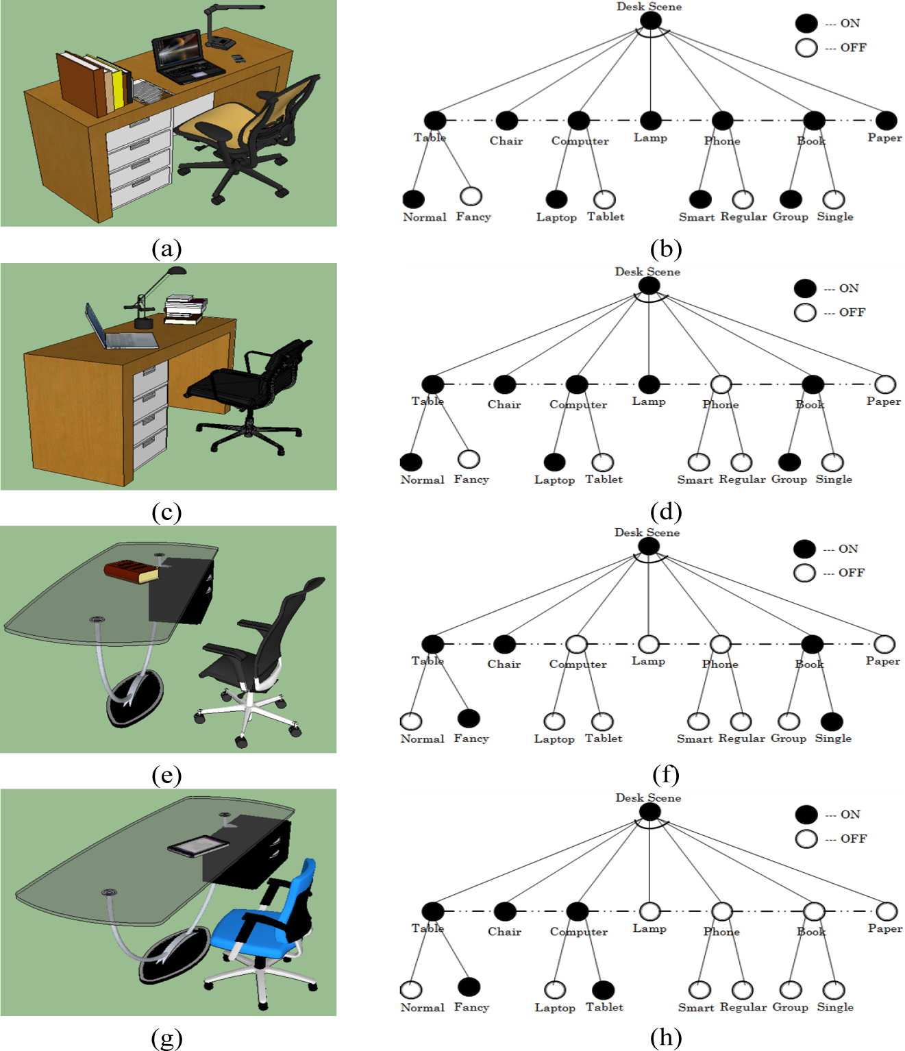
In our specific example, the And-Or graph represents desk scenes whose nodes are objects that constitute the scene. We can generate a large number of And-Or graphs to represent desk scenes by allowing the nodes to be sampled as either ON or OFF. This indirectly represents the relevancy of objects in the scene. As an example, we represent the desk scenes by composing a maximum of seven objects (i.e., those seen at least once in the training set) that are connected by dotted lines. These dotted lines, indicating the existence of an And relationship, enforce different contextual constraints such as relative position and orientation between objects. Furthermore, some of these nodes are represented as an Or node, indicating the variation in objects’ style as observed in the training examples; see Figure 1.
Assuming that the nodes in the And-Or graphs are identified for a given scene, 3D scene generation reduces to parsing the graph by first sampling the existence of each object based on their relevancy to the scene. Then, for each object with style variations (Or nodes), a style is sampled based on its probability as observed in the training examples. Finally, contextual constraints between the nodes that are turned ON are enforced. As an example, the first stage defines the existence of objects as: “The desk scene contains table, chair and computer”. The second stage defines the style of objects that are turned ON from the first stage as: “The desk scene contains a fancy table, a chair and a laptop computer”. The final stage enforces contextual constraints between the objects defined from the previous stages as: “The desk scene is arranged such that the laptop computer is at the center of a fancy table and the chair is in front of the fancy table”.
In this paper, a single instance of every node is considered. However, the number of instances of each node can also be considered as a variable. In such cases, it can integrated in the And-Or graph and be sampled during scene generation [7].
In order to represent 3D scene generation with And-Or graphs as discussed before, we define the tuple
where represents the nodes (i.e., objects) defined in the scene, represents a set of contextual constraints defined between the nodes, and represents a probabilistic distribution defined on the graph.
Each node ν ∈ is defined as
where e ϵ {0,1} (ON or OFF) represents the existence of object o; s ∈ {1, …,|s(o)|} represents the style of object o; and ϕ(o) represents physical attributes (position, scale and orientation) of the object o. Moreover, ϕ(o) = [p, σ, θ], where p = (x, y, z) marks the centroid of the object, σ = (σL, σW, σH) represents the dimensions of the bounding box, and θ represents the orientation of the object as projected onto the XY-plane. In our implementation, we extract seven unique object categories with a maximum of two styles.
3.2. Constraints
The following constraints are used in the MaxEnt model selection criterion to sample scenes from a Gibbs distribution.
3.2.1. Relevancy Constraint
In order to allow the sampling of nodes as ON or OFF, we learn the objects’ relevancy to the scene. To incorporate this constraint in our model, we compute a relevancy term using the object existence information from the training examples. This constraint is then used to sample an And-Or graph for a given scene.
Given the existence of each object as ON or OFF, the relevancy of an object can be computed as:
where e (o, i) represents the existence of object o in scene i, | | represents the total number of scenes ( ) and |V| is the total number of unique objects observed in the training examples. For the example shown in Figure 1, in which there are four training or observed scenes, one can compute table = 1 and paper = 0.25. This indicates that during scene generation, all of the synthesized scenes must have a table and 25% of the synthesized scenes are expected to have a paper. The observed constraint is therefore used to define the relevancy of objects in the synthesized scenes.
3.2.2. Hierarchical Constraint
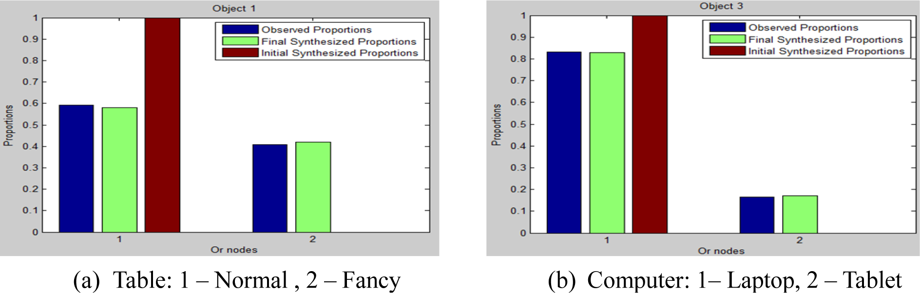
The hierarchical constraint is used to incorporate intra-class variations of object styles for scene generation, and it is represented by the Or-nodes in the graph. By counting the frequency of a given object style is observed from the training data, we can synthesize scenes that obey this style proportion.
Using object existence information as well as the corresponding style used in a given scene, we can define the proportion of object o appearing with style j, where j is style index, as:
where the Dirac-Delta function δ() will be unity only when object o is observed to have style j in scene i. For the training examples shown in Figure 1, we can compute computer(tablet) = 1/3 and computer(laptop) = 2/3 This term encodes the probability of sampling a given style of an object during scene generation.
In our experiment, since we consider at most a two-category style of objects, has a maximum of two dimensions for every object categories.
3.2.3. Contextual Constraint
Objects in a given scene are assumed to be constrained contextually by design preferences and/or physical constraints. The contextual pattern of the underlying constraint can be learned from training examples and can be used to generate plausible synthetic scenes. In our approach, we defined a set of pairwise contextual sub-constraints as shown in Table 1. To capture the multimodal nature of the contextual sub-constraints extracted from training samples, these sub-constraints are modeled with histograms. We assume that the pairwise sub-constraints defined in Table 1 are enough to extract the arrangements of objects from the training examples. In addition to the constraints defined in Table 1, we also use other indirect contextual constraints (i.e., intersection and visual balance) that are discussed in Section 4.
Histograms are extracted for each contextual sub-constraints defined in Table 1 as:
where l represents the contextual sub-constraint index, i refers to the bin location in the histogram, # is a counting function, #(rl(ϕo, ϕo′) = b) counts values falling in bin i and #(rl(ϕo, ϕo′)) counts values falling in any bin of the histogram for sub-constraint i. Here, Cl is modeled by a 32-bin histogram, resulting in a total of histograms representing the contextual constraint.
3.3. Maximum Entropy Framework
In our approach, we use the MaxEnt model selection criteria to identify a probability distribution that best fits the constraints extracted from the training set.
As Jaynes stated in [13], with the availability of limited information to select a generative probability distribution of interest, one can employ a variety of model selection strategies, of which the maximum entropy criterion is proven to be the most reliable and the least biased. This model selection criterion is briefly described below.
Given an unobserved true ( ) that generates a particular scene ( ) an unbiased distribution ( ) that approximates ( ) is the one with maximum entropy, satisfying the constraints simultaneously [13]. Using a set of constraints that can be extracted from the training scenes as observed constraints of, ( ) an unbiased probability distribution is selected using the MaxEnt criterion as follows:
Solving the above constrained optimization problem results in the following Gibbs distribution [13,14]:
where:
Here, represents the Lagrange multipliers.
Comparing the energy term ε( ; Λ) in Equation (7) with similar models used in [3,4], the first two terms in our model are Context-Free-Grammar and the third term is a Context-Sensitive-Grammar (Markov Random Field (MRF)). Our Context-Free-Grammar term captures the variability in terms of object’s relevance and style by pooling long-range relationships from many scenes. On the other hand, the MRF component enforces local contextual constraints within each scene, representing the short-range relationships. A more detailed explanation of the MRF component for scene generation is described in our previous work [1].
In order to sample from the Gibbs distribution given in Equation (7), the Λ parameters must first be determined. In [14,15], these parameters are learned using a gradient descent technique.
3.4. Parameter Estimation
The parameters of the Gibbs distribution is computed iteratively for each constraint as
where η represents the learning rate.
In order to learn parameters, scenes must be sampled by perturbing the objects’ relevancy ( ), style assignments ( ) and spatial arrangement ( ), respectively.
Computing the parameters for relevancy, hierarchical and contextual simultaneously is computationally expensive. As a result, these constraints are decoupled in such a way that we first sample scenes to obey the relevancy constraints. Once the relevancy constraint is obeyed, we sample the hierarchical constraints for objects that exist in each scene. Finally, scenes are sampled to capture the contextual constraints observed from the training examples. With each type of constraint, a greedy parameter optimization approach called feature pursuit [6,7,15] is followed that iteratively picks a single sub-constraint and updates the corresponding parameter while fixing the remaining parameters. This optimization approach is described next.
3.5. Feature Pursuit
As discussed, we use three types of constraints (relevancy, hierarchical and contextual), each of which is represented by multiple sub-constraints, specifically, | | sub-constraints for relevancy, | | sub-constraints for hierarchical and | | sub-constraints for contextual; see Equation (8). The parameters for these sub-constraints must be learned in order to match the constraints with those from the training examples. This is accomplished by the feature pursuit strategy.
In feature pursuit strategy, sub-constraints are selected one at a time from the pool of c sub-constraints. The selected sub-constraint is optimized until the divergence between the true distribution and that obtained from the approximate distribution reaches a minimum value.
The scene synthesis procedure is initialized by random sampling. Thereafter, a sub-constraint c+ is selected by first computing the squared Euclidean distance followed by picking the most diverging sub-constraint as given in Equations (9) and (10); respectively:
Where M ϵ {R, H, C}.
The corresponding parameter for the sub-constraint c+ is then learned iteratively using Equation (8) until its deviation is minimal. If through the selection process a sub-constraint is reselected, the estimated parameter values from the last selection are used to initialize the corresponding values in the new optimization cycle.
The intuition behind the feature pursuit strategy is that the sub-constraint with the highest deviation between the true and the approximate distributions should be prioritized and learned in order to bring the two distributions as close as possible.
As more sub-constraints are selected, more parameters are tuned and the sampled scenes come to resemble the patterns observed in the training scenes.
3.6. Sampling
In order to sample from the Gibbs distribution defined in Equation (7), a Metropolis sampling technique [16,17] is used. In Metropolis sampling, a new scene configuration is proposed by randomly picking a scene c from the synthesized scenes and perturbing the configuration with respect to the selected sub-constraint c+
as given by Equation (10). After the perturbation, the corresponding sub-constraints for the new configuration are extracted and the probability is evaluated. The transition to the new configuration ( → *) is then accepted with a probability of α such that:
where and are the probability of the old ( ) and the new (S*) configurations, respectively, as computed by Equation (7).
To give an example, assuming that we are working on contextual constraints (M = C) and the selected sub-constraint c+ (from Equation (10)) is the relative position of table to chair in the x-axis, the corresponding λ parameter is first estimated using Equation (8). A scene is randomly picked from the synthesized scenes and a new configuration is proposed by perturbing the position of either the chair or the table along the x-axis (sampled uniformly from a specified range of positions). Using the sub-constraints extracted after the perturbation and the λ parameter, the probability is computed using Equation (7). The new configuration is then either accepted or rejected depending on the acceptance probability computed using Equation (11).
The sampling, feature pursuit, and parameter estimation are continuously applied until the energy overall divergence between the two distribution constraints, as given by Equation (12), is minimal.
Given a set of training scenes SF, we can generate a set of synthetic scenes SP using the pseudocodes shown in Algorithm 1 and Algorithm 2. In our implementations, we have used ϵ1 = 0.1, ϵ2 = 0.1 and η = 1
4. Implementation
In this section, we explain the implementation details for generating plausible and visually appealing synthetic scenes using the proposed approach.
4.1. Additional Contextual Constraints
In addition to the constraints mentioned earlier, we also considered criteria that help to make the synthesized scenes more plausible and visually appealing. These considerations are detailed next.
4.1.1. Intersection Constraint
The model described thus far has no provisions for prohibiting the occurrence of intersecting objects. To remedy this shortcoming, we incorporate the intersection constraint, which uses the projection of object’s bounding box on the XY-plane (top-view of the scenes). For every pair of objects o and o′ the intersection constraint is defined as:
where Axy(o ∩ o′) is the area of the intersection on the XY-plane between pairs of objects, and Axy(o) is the area of the object o. Defined in this way, the intersection term ϑ(o,o′) will have a value between 0 and 1, where 0 indicates no intersection and 1 indicates that object o is contained in object , as viewed from the top. Ideally, two objects should not intersect unless there is a parent-child support. During scene perturbation, setting the intersection threshold too close to zero causes a significant computational cost since random perturbations often produce intersecting objects. On the other hand, setting this threshold too close to one allows objects to intersect with each other, resulting in a large number of implausible scenes. We, therefore, experimented with this value and found 0.1 to be a reasonable compromise for the desk scene example.
While intersection can be encoded as a soft constraint in the energy expression (e.g., see [11]), it is used here as a hard constraint defined in the scene perturbation step. If the perturbed configurations result in intersecting objects (the intersection ratio is above the predefined threshold of 0.1), it is discarded and the scene is perturbed again. This process is repeated until the intersection between objects in a given scene is below the threshold. In addition to playing a role in the scene perturbation process, as described in the next section, the intersection constraint is utilized to identify the parent-child support between objects by integrating it with object contact information.
4.1.2. Parent-Child Support
To demonstrate the parent-child support criteria, consider a laptop placed on a table. Usually, the laptop is contained in the table, as seen from the top view (XY projection of the scene) and it is in contact with the table if viewed from the side. The contact constraint, formulated by Equation (14), is expected to be very small for two objects with a parent-child relationship.
Where minz(o) is the height of the bottom (minz) surface of object o and maxz(o′) is the height of the top (maxz) surface of object o′.
Using Equations (13) and (14), it can be computed that ϑ(laptop, table) =1 (assuming the laptop is completely contained in the table) and ζ(laptop, table) ≅ 0. These two results indicate that table is a parent of laptop, or conversely, laptop is a child of table. After identifying the parent-child support relations from the set of training examples, every child object is set to be placed on top and within the boundary of its parent object during scene synthesis. Objects that do not have a parent (for example chair or table) are set to lay on the floor, and their position is sampled on the XY plane inside a room with pre-specified dimensions. Using our training examples, it is identified that that computer, phone, paper, book and lamp are the children of table and, therefore, their centroid position on the XY plane is sampled within the boundary of their parent.
In this section, parent-child support is formulated based on the assumption that child objects normally exist on top of the bounding box of their parent. Although this is a valid assumption for the training scenes that are used in our experiment, it will fail for the general case when a parent object has many supporting surfaces. As a result, this assumption needs to be relaxed by first segmenting out any supporting surfaces of a given object and evaluating the parent-child relationship on each surface. During scene generation, this will add additional contextual constraints on the height of objects (along the Z-axis). Therefore, the height of each object can also be sampled in a similar fashion as the relative position along the X- and Y-axis.
4.1.3. Visual Balance
Unlike the intersection constraint that restricts the synthesis of intersecting objects, visual balance, which largely depends on personal preference, is implemented as a soft constraint. As a result, the visual balance constraint is incorporated on children objects by modifying the energy expression defined in Equation (7) as:
Here,εvb is the visual balance cost, and wvb determines how much this term should influence the scene generation. In [10] Merrell et al. incorporated a visual balance criterion over a single scene containing furniture objects to be arranged in a room. Here, the visual balance criterion defined in [10] is adapted for a set of scenes with a parent-child support as given by:
where ρ refers the parent object, τ(o,ρ) ∈ {0,1} is an indicator function and it will be 1 if ρ is a parent of o, is the (x, y) position of object o, is the (x, y) position of the parent, ‖⋅‖ is the norm operator and |SP| is the number of synthesized scenes.
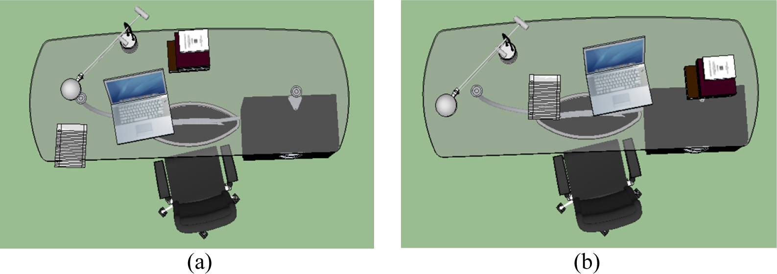
To clarify what εvb is measuring, compare the scene shown in Figure 2a with that in Figure 2b. In Figure 2a, the child objects are aggregated to one side resulting in an unbalanced “load” across the table. As a result, this is considered to be an unbalanced scene incurring a higher visual balance cost (computed to be 15.7 using Equation (16) for a single scene). On the other hand, child objects are more evenly distributed across the table in Figure 2b resulting in a much lower visual balance cost (similarly computed to be 0.5). As a result, the visual balance cost favors a more balanced arrangement of children objects.
The reason for handling visual balance as an energy term (as opposed to incorporating it into the model as an additional contextual sub-constraint) is that the visual balance constraint adds significant complexity to the feature pursuit procedure. To clarify, if for example the maximum deviating sub-constraint in feature pursuit happens to be relative position in the X-axis between lamp and paper, either of the objects can be perturbed along the X-axis and decide whether to accept or reject the proposed configuration. However, visual balance depends on not just a pair of objects, but on all children objects. Moreover, visual balance can be modified by perturbing a large combination of constraints.
Note that since all the other constraints are normalized counts, the weight should be set to a small value to avoid overweighting this constraint as compared to the other contextual constraints. In our experiments, we have used wvb = 0.05
4.1.4. Front and Back Side Determination
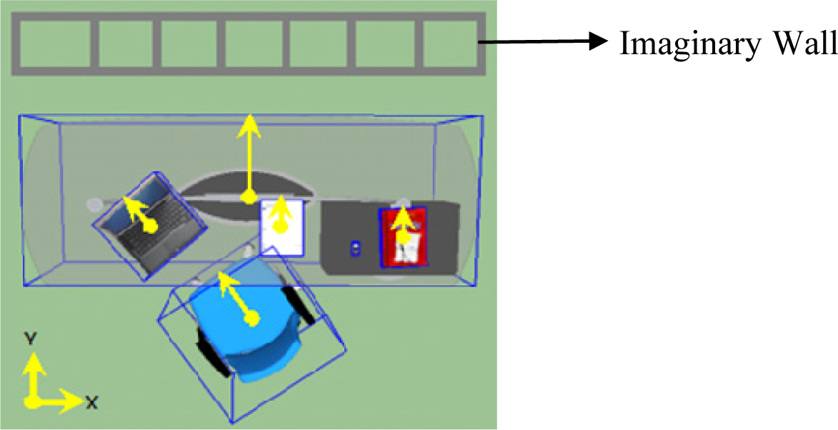
In order to synthesize scenes with the appropriate orientation of objects, the scene generation approach should incorporate a way to identify the front versus the back sides of objects. In Yu et al. [11], the back side of an object is determined by first computing the distance from each side of the object to the nearest wall and selecting the side with smallest distance. Here, since the training scenes do not contain walls, we defined an imaginary wall and extract the orientation of each object. The imaginary wall is defined parallel to the X-axis and is set to lay above all the existing objects in the positive Y-axis in every scene; see Figure 3. Using this imaginary wall, the back side is defined to be the nearest side of the object to the wall (by computing the midpoints of each side and selecting the side having the maximum y value). The chair is of course treated differently as it normally faces the table and as a result, its nearest side to the wall is the front side. Once the proper side for each object is detected, a vector originating from the centroid to the detected side of each object is defined; see Figure 3. The angle between the vector and the positive Y-axis is computed and used as the orientation feature for objects. For synthesis, object models are manually oriented to zero degrees (i.e. their back side faces the positive Y-axis, except for the chair). The sampled orientation using our framework is then applied to generate the synthetic scenes.
4.2. Scene Initialization and Perturbation
In the proposed framework, |SP| = 50 initial synthetic scenes are randomly sampled. In all of these scenes, the relevancy of each object is assumed unity, which resulted in placing every object in every scene, i.e.. For objects with multiple styles, the first style is the one selected for initialization and the corresponding dimensions are assigned as σ = (σL, σW σH) For objects with no parents (such as table or chair) the positional features are randomly sampled to any location in the room, i.e.,x = rand (σRoom), and y = rand (σRoom), where σRoom is set to 500 ft; the centroid along the Z-axis is obtained from the height of the object, i.e., ; and the orientation is sampled as On the other hand, for child objects their positional features are contained in and supported by their parents, i.e., x = rand(σρ,x), and y = rand(σρ,y), where σρ,x and σρ,y are the extents of the parent along the X and Y axes; the centroid along the Z-axis is computed as the height of the parent plus half of that of the object, i.e., ; and the orientation is initialized as .
Once the scenes are randomly initialized, they are then perturbed and sampled to ultimately match the constraints extracted from the training examples. Depending on the type of constraint being optimized, the scene perturbation is performed as follows. If relevancy constraint is selected ( ) for a given sub-constraint c+ a scene & is randomly picked from the synthesized scenes SP. Then, the existence of the object in scene c corresponding to c+ is randomly sampled as e = rand{0,1} and the probability of the new configuration is either accepted or rejected based on Equation (13).
Similarly, if hierarchical constraint is selected ( = ) for a given sub-constraint c+, a scene & is randomly picked from the synthesized scenes SP. Then, the style of the object in scene & corresponding to c+ is randomly sampled as s = rand (|s(ok)|) and the configuration is updated according to Equation (13).
Finally, if contextual constraint is selected ( = ) for a given sub-constraint c+, a scene & is randomly picked from the synthesized scenes Ssyn* in which both objects (o and o′) expressed by c+ exist. Then, one of the objects (either o or o′) is randomly picked and the corresponding feature expressed in c+ is perturbed. Since we have defined the intersection constraint as a hard constraint, the perturbed object’s feature is used to check if the intersection ratio with any other object in that scene is below the defined threshold. If any of the intersection ratios falls above the threshold, the perturbation is discarded and a new sample is generated. This procedure is repeated a maximum of = 250 iterations and is either accepted or rejected based on Equation (13). The perturbations are defined as:
For child object:
- ○
For relative position in X, x = rand (σρ,x)
- ○
For relative position in Y, y = rand (σρ,y)
- ○
For relative orientation, .
For non-child object:
- ○
For relative position in X, x = rand (σRoom)
- ○
For relative position in Y, y = rand (σRoom)
- ○
For relative orientation, .
5. Results
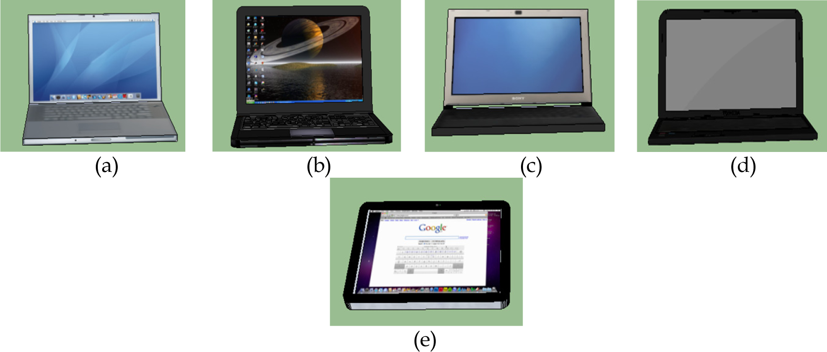
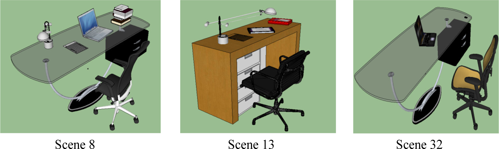
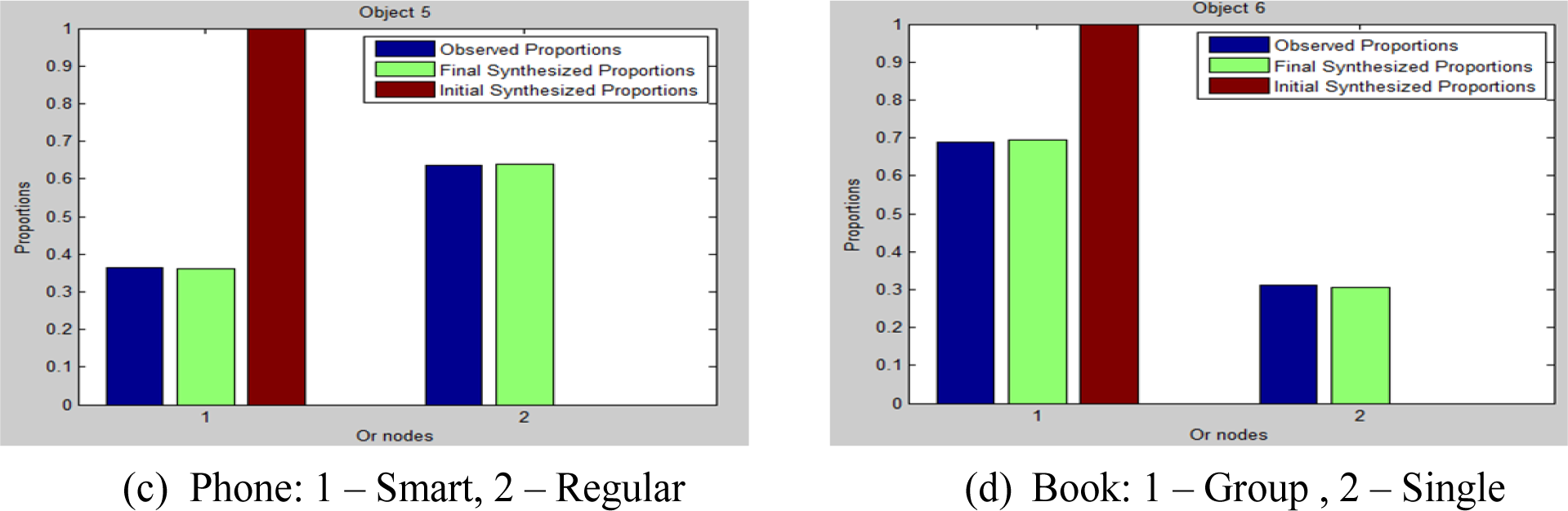
In this section, we present the results from the proposed MaxEnt based scene generation framework. Our training dataset contains |SF| = 22 manually designed desk scenes with different object existence, styles, position and orientation; four of these training scenes are shown in Figure 1. These training scenes are designed using the models as described in Table 2. To help visualizing what is described in Table 2, we included the different 3D models used to represent computers in Figure 4. During scene synthesis, we considered every object model of a given style to have equal probability and a model is sampled uniformly.
Using the training examples, a set of relevancy, hierarchical and contextual constraints are extracted and used as observed constraints to sample a set of synthetic scenes. As described in Section 3.4, we decouple these constraints in such a way that we first sample scenes to obey the relevancy constraint. Once this is accomplished, we sample the hierarchical constraints for objects that exist in each scene. Finally, scenes are sampled to capture the contextual constraints observed from the training examples.
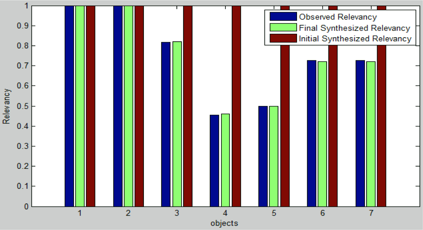
Once the relevancy constraints are extracted from the training and a synthetic scene, feature pursuit is applied by continuously sampling the existence of the objects in the synthetic scenes and updating the parameters until the divergence is minimal. The result of this procedure can be seen in Figure 5, which indicates that the relevancy constraint between training and synthetic scenes is matched at the end of this step.
After the relevancy constraint is matched, the hierarchical constraint is optimized until the objects’ style proportion is matched for those with multiple styles; see Figure 6. For objects with a single style (chair, lamp and paper in our example), there is no Or-node defined and, therefore, the proportion is not changed. Again, we can see from Figure 6 that our proposed framework is able to match the hierarchical constraints by sampling the objects’ style variations.
After both the relevancy and hierarchical constraints are satisfied, the final step is imposing contextual constraints on the synthetic scenes. Using the pairwise relations defined in Table 1, a total of 63 () contextual constraints (i.e., histograms with 32 bins) are extracted from the training as well as the synthetic scenes. Subsequently, feature pursuit is applied to match the sets of contextual constraints to produce the final scenes as shown in Figure 7.
It can be seen from Figure 7 that the proposed framework is able to learn from the training data and generate scenes that capture the observed relevancy, style and contextual variations.
5.1. Analysis
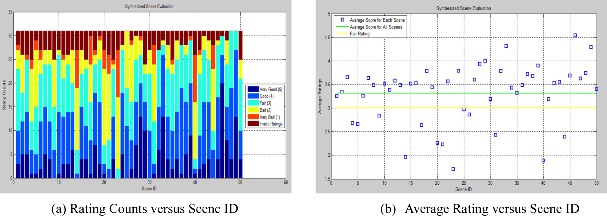
To assess the performance of our proposed framework, 31 test subjects were first shown a few scenes from the training data to establish a reference for scene acceptability. Thereafter, they were presented the 50 synthesized scenes and were asked to rate each scene into five categories: Very bad (1), bad (2), fair (3), good (4) and very good (5). Furthermore, for better understanding of the ratings, the participants were asked to justify their rating. The ratings were then consolidated and are represented in Figure 8. In the color-bar graph of Figure 8a, we have added a rating termed as “invalid rating”. This represents unexpected responses from the participants (such as “awkward viewpoint”, and “the paper is too dark”) that are discarded while computing the average ratings per scene shown in Figure 8(b). It is observed that only 26% of the scenes are rated as implausible (defined as a rating of less than fair) by the observers; see Figure 8b.
We would like to mention that our objective here is not so much to quantify the plausible scenes but rather to quantify the implausible ones, as we would expect less inter-subject variability in the latter than the former. This allowed us to quantify and report our approach’s tendency to generate implausible scenes.
5.2. Comparison with Existing Approach
In Section 2, we mentioned the advantage of the MaxEnt framework over the existing approaches for scene generation application. In comparison with the MaxEnt framework, the existing approaches [10,11,12] optimize a single output scene in one run of their algorithms. A potential problem with these approaches is that since each synthesized scene is optimized independently using the same constraints, they often sample the most probable object arrangements. As a result, the range of variations of the output scenes is small.
Among the existing approaches, Fisher et al. [12] work is the most recent and has a significant overlap with our proposed approach. As a result, we compare the MaxEnt framework with the work of Fisher et al. [12] using a 3D dining scene. For this comparison, we only considered the arrangement model of Fisher et al. [12] with our contextual framework, assuming that the number of objects and their styles are predefined in both approaches.
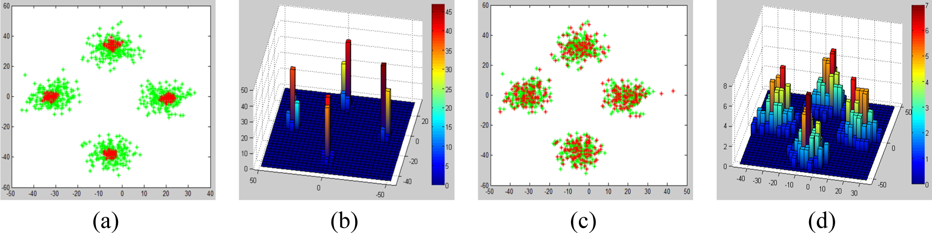
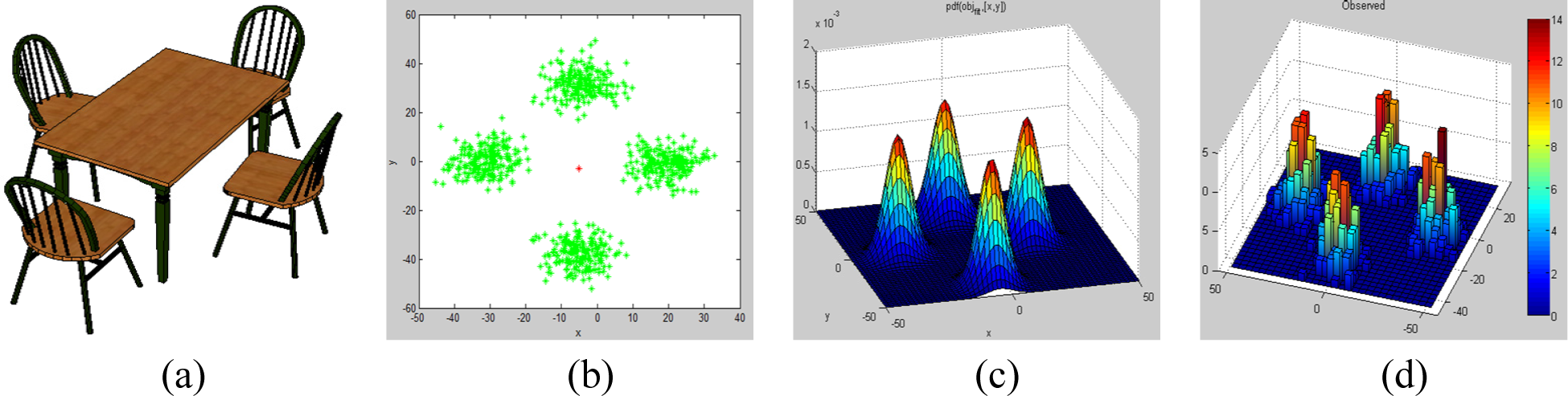
Given a sample training scene shown in Figure 9a, the centroid of each object along X and Y axis is extracted. As proposed by Fisher et al. [12], the training scene shown in Figure 9a is amplified to 200 scenes. To amplify the size of the training data, the positions of the chairs are jittered by sampling from a bivariate Gaussian distribution with zero mean and a variance of 5 inches; see Figure 9b. Thereafter, Fisher et al. [12] represented the training data by a conditional Probability Density Function (PDF) using Gaussian Mixture Models (GMM); see Figure 9c. In our approach, we represent the training data by a 2D histogram; see Figure 9d.
In order to synthesize new scenes, Fisher et al. [12] defined a layout score that integrates the conditional PDF of pair of objects with collision, proximity and overhang penalty. These penalty terms prevent objects from penetrating and colliding with each other as well as levitating in the air.
Thereafter, scene generation procedure is implemented in Fisher et al. [12] as follows. Starting from a random configuration of objects in a single scene, object’s position is iteratively perturbed and the layout score is computed. The perturbed scene is accepted when the layout score is maximized. This procedure is repeated until a certain stopping criterion is reached; here a maximum number of iteration is used as a stopping criterion. In Figure 10, a sample scene synthesis procedure as proposed in [12] is shown. As it can be seen from this figure, the layout score is maximum when the chair positions are arranged around the peak of each Gaussian in the GMM.
On the other hand, the scene generation procedure in our approach is implemented as follows. First, the energy term of the Gibbs distribution defined in Equation (7) is redefined using the 2D histogram and additional terms to incorporate proximity, collision and overhang penalties. Using the observed scenes shown in Figure 9b, a bivariate histogram is extracted; see Figure 9d. Thereafter, multiple synthesis scenes (set to 100) are initialized and the corresponding histogram is extracted; see Figures 11a,b. As expected, the initial scenes are random and uniformly distributed in both dimensions. Under the MaxEnt framework, synthesis scenes are perturbed and updated until the observed histogram matches the synthesis histogram while obeying the penalties. As the optimization converges, the distribution of the synthesis scenes matches that of the observed scenes; see Figures 11c,d.
In order to compare the approach proposed by Fisher et al. [12] with MaxEnt framework, one needs to generate equal number of scenes and analyze the distribution of the scenes. Since Fisher et al. [12] approach generates a single synthesis scene at a time, their algorithm is run 100 times to generate 100 scenes. On the other hand, the MaxEnt framework synthesizes multiple instances and a single run is enough since the number of synthesis scenes is set to 100. The output of the two approaches is compared by fixing the number of iteration in each optimization to 1000; see Figure 12.
From these figure, one can see that Fisher et al. approach synthesizes most of the scenes at the peak of the Gaussians in GMM; see Figures 12a,b. As a result, the variability of the scenes generated from their approach has a small variability. On the other hand, the scenes generated with the MaxEnt framework have a larger variability and it captures the observed distribution very well; see Figures 12c,d.
6. Conclusions
In this paper, we proposed a novel automatic, data-driven 3D scene generation framework based on MaxEnt model selection criterion. Unlike the existing methods, our framework incorporates relevancy, hierarchical and contextual constraints into a unified framework. By integrating the relevancy constraint into the model, our approach manages to sample from multiple, conceptually-similar And-Or graphs, allowing variability in terms of object existence.
In addition to introducing a relevancy constraint into a hierarchical and contextual MaxEnt framework, we incorporated different contextual constraints namely: Intersection constraint, parent-child support and visual-balance criteria. As a result, the proposed approach is capable of generating plausible synthetic scenes with wide range of variations.
In order to evaluate the plausibility of the scenes generated using the proposed framework, we gathered feedback from human graders. Form this evaluation procedure, more than 70% of the scenes are rated above fair and the average rating of all scenes is obtained to fall above fair. This evaluation confirms that the proposed framework is capable of generating a reasonable number of plausible scenes automatically.
Thereafter, a comparison of the proposed framework with the existing approaches is discussed. During the comparison, it is demonstrated that the proposed framework captures the variability of the observed scenes and generate scenes with larger variability as compared with the existing approaches.
As a final note, although the applicability of the proposed approach is illustrated with only an exemplary desk scene in this paper, the framework can be used to synthesize any scene. Given a scene that is composed of objects/parts and constrained by relevancy, hierarchical and contextual constraints, the same process detailed in Algorithms 1 and 2 can be readily used to generate synthesized scenes. For example, suppose we want to utilize the proposed framework to synthesize plausible living room scenes by arranging furniture objects such as couches, tables, a TV set, side-tables, etc. As illustrated in this paper, first, a set of training living room scenes are collected and parsed to extract the objects in the scene, their styles, as well as their relative position and orientation. This observed information is then represented by histogram constraints. Thereafter, similar to the desk scene example, a set of randomly synthesized living room scenes are generated and their corresponding histograms are extracted. Finally, the synthesized scenes are perturbed and updated until their histograms converge to the observed histograms.
Author Contributions
The authors contributed equally in conceiving, designing and analyzing the approach as well as preparing this manuscript.
Conflicts of Interest
The authors declare no conflict of interest.
References
- Dema, M.A.; Sari-Sarraf, H. A maximum entropy based data-driven 3D scene generation. Int. J. Semantic Comput 2013, 7, 69–85. [Google Scholar]
- Dema, M.A.; Sari-Sarraf, H. 3D scene generation by learning from examples, In Proceedings of the IEEE International Symposium on Multimedia (ISM), Irvine, CA, USA, 10–12 December 2012; pp. 58–64.
- Zhu, S.C.; Mumford, D. A stochastic grammar of images. Foundation and Trends in Computer Graphics and Vision 2006, 2, 259–362. [Google Scholar]
- Chen, H.; Xu, Z.; Liu, Z.; Zhu, S.C. Composite templates for cloth modeling and sketching. CVPR 2006, 1, 943–950. [Google Scholar]
- Xu, Z.; Chen, H.; Zhu, S.C.; Luo, J. A hierarchical compositional model for face representation and sketching. IEEE Trans. Pattern Anal. Mach. Intell 2008, 30, 955–969. [Google Scholar]
- Porway, J.; Yao, B; Zhu, S.C. Learning compositional models for object categories from small sample sets. In Object Categorization: Computer and Human Vision Perspectives; Dickson, S.J., Leonardis, A., Schiele, B., Tarr, M.J., Eds.; Cambridge Press: New York, NY, USA, 2009; pp. 241–256. [Google Scholar]
- Porway, J.; Wang, Q.; Zhu, S.C. A hierarchical and contextual model for aerial image parsing. Int. J Comput. Vision 2010, 88, 254–283. [Google Scholar]
- Chaudhuri, S.; Kalogerakis, E.; Guibas, L.; Koltun, V. Probabilistic reasoning for assembly-based 3D modeling. ACM Trans. Graph 2011, 30, 35:1–35:10. [Google Scholar]
- Kalogerakis, E.; Chaudhuri, S.; Koller, D.; Koltun, V. A probabilistic model for component-based shape synthesis. ACM Trans. Graph. 2012, 31, 55:1–55:11. [Google Scholar]
- Merrell, P.; Schkufza, E.; Li, Z.; Agrawala, M.; Koltun, V. Interactive furniture layout using interior design guidelines. ACM Trans. Graph 2011, 30, 87:1–87:10. [Google Scholar]
- Yu, L.; Yeung, S.; Tang, C.; Terzopoulos, D.; Chan, T.F.; Osher, S.J. Make it home: Automatic optimization of furniture arrangement. ACM Trans. Graph 2011, 30, 86:1–86:11. [Google Scholar]
- Fisher, M.; Ritchie, D.; Savva, M.; Funkhouser, T.; Hanrahan, P. Example-based synthesis of 3D object arrangements. ACM Trans. Graph 2012, 31, 135:1–135:11. [Google Scholar]
- Jaynes, E. Discrete prior probabilities: The entropy principle. In Probability Theory: The Logic of Science; Bretthorst, G.L., Ed.; Cambridge Press: Cambridge, UK, 2003; pp. 343–371. [Google Scholar]
- Malouf, R. Maximum entropy models. In Handbook of Computational Linguistics and Natural Language Processing; Clark, A., Fox, C., Lappin, S., Eds.; Wiley Blackwell: West Sussex, UK, 2010; pp. 133–155. [Google Scholar]
- Zhu, S.C.; Wu, Y.; Mumford, D. Filters, Random Fields and Maximum Entropy (FRAME): Towards a unified theory for texture modeling. Int. J. Comput. Vision 1998, 27, 1–20. [Google Scholar]
- Walsh, B. Markov Chain Monte Carlo and Gibbs Sampling, Available online: http://citeseerx.ist.psu.edu/viewdoc/summary?doi=10.1.1.131.4064 (accessed on 8 May 2014).
- Rutenbar, R.A. Simulated annealing algorithms: An overview. IEEE Circ. Dev. Mag 1989, 5, 19–26. [Google Scholar]


| Relationships (r) | Formula |
|---|---|
| Relative position in X axis | xo−xo′ |
| Relative position in Y axis | yo−yo′ |
| Relative Orientation | θo−θo′ |
| Object ID | Object Name | Models used for each styles | |
|---|---|---|---|
| Style 1 | Style 2 | ||
| 1 | Table | 1 | 1 |
| 2 | Chair | 5 | - |
| 3 | Computer | 4 | 1 |
| 4 | Lamp | 3 | - |
| 5 | Phone | 1 | 1 |
| 6 | Book | 2 | 2 |
| 7 | Paper | 1 | - |
| 1 | function SP= Synthesize_Scenes(SF) |
| 2 | // Input: A set of training scenes SF |
| 3 | // Output: A set of synthetic scenes SP |
| 4 | – Initialize synthetic scenes SP |
| 5 | – SP = Constrain_Scenes (SP, SF,M = R) |
| 6 | – SP = Constrain_Scenes (SP, SF,M = H) |
| 7 | – SP = Constrain_Scenes (SP, SF,M = C) |
| 1 | function SP = Constrain_Scenes (SP, SF, M) |
| 2 | – Using all training scenes SF extract constraints MF |
| 3 | – Using all synthetic scenes SP extract constraints MP |
| 4 | – Initialize λ =0, where λ ∈ Λ |
| 5 | – Repeat |
| 6 | – Compute using (9) |
| 7 | – Select a constraint c+ using (10) |
| 8 | – Repeat |
| 9 | – Update λ for constraint c+ using (10) |
| 10 | – Initialize SP* by SP |
| 11 | – For i=1:Iter_Max |
| 12 | – Pick a synthetic scene & uniformly from SP* |
| 13 | – Perturb & for c+ and propose SP* (See Section 4.2) |
| 14 | – Extract MP* |
| 15 | – Compute using (9) |
| 16 | – Compute α(SP→SP*) using (13) |
| 17 | – Draw a random number uniformly rand ϵ [0,1] |
| 18 | – If rand ≤ α(SP→SP*) |
| 19 | SP←SP* |
| 20 | MP←MP* |
| 21 | Else |
| 22 | SP*←SP |
| 23 | – Compute for constraint c+ using (11) |
| 24 | – Until < ϵ1 |
| 25 | –Until < ϵ2 using (12) |
© 2014 by the authors; licensee MDPI, Basel, Switzerland This article is an open access article distributed under the terms and conditions of the Creative Commons Attribution license (http://creativecommons.org/licenses/by/3.0/).
Share and Cite
Dema, M.; Sari-Sarraf, H. A Relevancy, Hierarchical and Contextual Maximum Entropy Framework for a Data-Driven 3D Scene Generation. Entropy 2014, 16, 2568-2591. https://doi.org/10.3390/e16052568
Dema M, Sari-Sarraf H. A Relevancy, Hierarchical and Contextual Maximum Entropy Framework for a Data-Driven 3D Scene Generation. Entropy. 2014; 16(5):2568-2591. https://doi.org/10.3390/e16052568
Chicago/Turabian StyleDema, Mesfin, and Hamed Sari-Sarraf. 2014. "A Relevancy, Hierarchical and Contextual Maximum Entropy Framework for a Data-Driven 3D Scene Generation" Entropy 16, no. 5: 2568-2591. https://doi.org/10.3390/e16052568