General H-theorem and Entropies that Violate the Second Law

Abstract
: H-theorem states that the entropy production is nonnegative and, therefore, the entropy of a closed system should monotonically change in time. In information processing, the entropy production is positive for random transformation of signals (the information processing lemma). Originally, the H-theorem and the information processing lemma were proved for the classical Boltzmann-Gibbs-Shannon entropy and for the correspondent divergence (the relative entropy). Many new entropies and divergences have been proposed during last decades and for all of them the H-theorem is needed. This note proposes a simple and general criterion to check whether the H-theorem is valid for a convex divergence H and demonstrates that some of the popular divergences obey no H-theorem. We consider systems with n states Ai that obey first order kinetics (master equation). A convex function H is a Lyapunov function for all master equations with given equilibrium if and only if its conditional minima properly describe the equilibria of pair transitions Ai ⇌ Aj. This theorem does not depend on the principle of detailed balance and is valid for general Markov kinetics. Elementary analysis of pair equilibria demonstrate that the popular Bregman divergences like Euclidian distance or Itakura-Saito distance in the space of distribution cannot be the universal Lyapunov functions for the first-order kinetics and can increase in Markov processes. Therefore, they violate the second law and the information processing lemma. In particular, for these measures of information (divergences) random manipulation with data may add information to data. The main results are extended to nonlinear generalized mass action law kinetic equations.1. The Problem
The first non-classical entropy was proposed by Rényi in 1960 [1]. In the same paper he discovered the very general class of divergences, the so-called f-divergences (or Csiszár-Morimoto divergences because of the works of Csiszár [2] and Morimoto [3] published simultaneously in 1963):
where P = (pi) is a probability distribution, P* is an equilibrium distribution, h(x) is a convex function defined on the open (x > 0) or closed x ≥ 0 semi-axis. We use here the notation Hh(P ∥P*) to stress the dependence of Hh on both pi and
These divergences have the form of the relative entropy or, in the thermodynamic terminology, the (negative) free entropy, the Massieu-Planck functions [4], or F/RT where F is the free energy. They measure the deviation of the current distribution P from the equilibrium P*.
After 1961, many new entropies and divergences were invented and applied to real problems, including Burg entropy [5], Cressie-Red family of power divergences [6], Tsallis entropy [7,8], families of α-,β- and γ-divergences [9] and many others (see the review papers [10,11]). Many of them have the f-divergence form, but some of them do not. For example, the squared Euclidean distance from P to P* is not, in general, a f-divergence unless all are equal (equidistribution). Another example gives the Itakura-Saito distance:
The idea of Bregman divergences [12] provides a new general source of divergences different from the f-divergences. Any strictly convex function F in an closed convex set V satisfies the Jensen inequality
if p ≠ q, p, q ∈ V. This positive quantity DF(p, q) is the Bregman divergence associated with F. For example, for a positive quadratic form F (x) the Bregman distance is just DF (p, q) = F (p − q). In particular, if F is the squared Euclidean length of x then DF (p, q) is the squared Euclidean distance. If F is the Burg entropy, , then DF (p; q) is the Itakura-Saito distance. The Bregman divergences have many attractive properties. For example, the mean vector minimizes the expected Bregman divergence from the random vector [13]. The Bregman divergences are convenient for numerical optimization because generalized Pythagorean identity [14]. Nevertheless, for information processing and for many physical applications one more property is crucially important.
The divergence between the current distribution and equilibrium should monotonically decrease in Markov processes. It is the ultimate requirement for use of the divergence in information processing and in non-equilibrium thermodynamics and kinetics. In physics, the first result of this type was Boltzmann’s H-theorem proven for nonlinear kinetic equation. In information theory, Shannon [15] proved this theorem for the entropy (“the data processing lemma”) and Markov chains.
In his well-known paper [1], Rényi also proved that Hh(P ∥P*) monotonically decreases in Markov processes (he gave the detailed proof for the classical relative entropy and then mentioned that for the f-divergences it is the same). This result, elaborated further by Csiszár [2] and Morimoto [3], embraces many later particular H-theorems for various entropies including the Tsallis entropy and the Rényi entropy (because it can be transformed into the form (1) by a monotonic function, see for example [11]). The generalized data processing lemma was proven [16,17]: for every two positive probability distributions P, Q the divergence Hh(P∥Q) decreases under action of a stochastic matrix A = (aij)
where
is the ergodicity contraction coefficient, . Here, neither Q nor P must be the equilibrium distribution: divergence between any two distributions decreases in Markov processes.
Under some additional conditions, the property to decrease in Markov processes characterizes the f-divergences [18,19]. For example, if a divergence decreases in all Markov processes, does not change under permutation of states and can be represented as a sum over states (has the trace form), then it is the f-divergence [11,18].
The dynamics of distributions in the continuous time Markov processes is described by the master equation. Thus, the f-divergences are the Lyapunov functions for the master equation. The important property of the divergences Hh(P∥P*) is that they are universal Lyapunov functions. That is, they depend on the current distribution P and on the equilibrium P* but do not depend on the transition probabilities directly.
For each new divergence we have to analyze its behavior in Markov processes and to prove or refute the H-theorem. For this purpose, we need a simple and general criterion. It is desirable to avoid any additional requirements like the trace form or symmetry. In this paper we develop this criterion.
It is obvious that the equilibrium P* is a global minimum of any universal Lyapunov function H(P) in the simplex of distributions (see the model equation below). In brief, the general H-theorem states that a convex function H(P) is a universal Lyapunov function for the master equation if and only if its conditional minima correctly describe the partial equilibria for pairs of transitions Ai ⇌ Aj. These partial equilibria are given by proportions . They should be solutions to the problem
These solutions are minima of H(P) on segments . They depend on n − 2 parameters .
Using this general H-theorem we analyze several Bregman divergences that are not f-divergences and demonstrate that they do not allow the H-theorem even for systems with three states. We present also the generalizations of the main results for Generalized Mass Action Law (GMAL) kinetics.
2. Three Forms of Master Equation and the Decomposition Theorem
We consider continuous time Markov chains with n states A1, …, An. The Kolmogorov equation or master equation for the probability distribution P with the coordinates pi (we can consider P as a vector-column P = [p1, …, pn]T is
where qij (i, j = 1, …, n, i ≠ j) are nonnegative. In this notation, qij is the rate constant for the transition Aj → Ai. Any set of nonnegative coefficients qij (i ≠ j) corresponds to a master equation. Therefore, the class of the master equations can be represented as a nonnegative orthant in ℝn(n−1) with coordinates qij (i ≠ j). Equations of the same class describe any first order kinetics in perfect mixtures. The only difference between the general first order kinetics and master equation for the probability distribution is in the balance conditions: the sum of probabilities should be 1, whereas the sum of variables (concentrations) for the general first order kinetics may be any positive number.
It is useful to mention that the model equation with equilibrium P* and relaxation time τ
is a particular case of master equation for normalized variables Indeed, let us take in Equation (7).
The graph of transitions for a Markov chain is a directed graph. Its vertices correspond to the states Ai and the edges correspond to the transitions Aj → Ai with the positive transition coefficients, qij > 0. The digraph of transitions is strongly connected if there exists an oriented path from any vertex Ai to every other vertex Aj (i ≠ j). The continuous-time Markov chain is ergodic if there exists a unique strictly positive equilibrium distribution for master Equation (7) [20,21]. Strong connectivity of the graph of transitions is necessary and sufficient for ergodicity of the corresponding Markov chain.
A digraph is weakly connected if the underlying undirected graph obtained by replacing directed edges by undirected ones is connected. The maximal weakly connected components of a digraph are called connected (or weakly connected) components. The maximal strongly connected subgraphs are called strong components. The necessary and sufficient condition for the existence of a strongly positive equilibrium for master Equation (7) is: the weakly connected components of the transition graph are its strong components. An equivalent form of this condition is: if there exists a directed path from Ai to Aj, then there exists a directed path from Aj to Ai. In chemical kinetics this condition is sometimes called the “weak reversibility” condition [22,23]. This implies that the digraph is the union of disjoint strongly connected digraphs. For each strong component of the transition digraph the normalized equilibrium is unique and the equilibrium for the whole graph is a convex combination of positive normalized equilibria for its strong components. If m is the number of these components then the set of normalized positive equilibria of master equation is a relative interior of a m − 1-dimensional polyhedron in the unit simplex ∆n. The set of non-normalized positive equilibria is a relative interior of a m-dimensional cone in the positive orthant .
The Markov chain in Equation (7) is weakly ergodic if it allows the only conservation law: the sum of coordinates, . Such a system forgets its initial condition: the distance between any two trajectories with the same value of the conservation law tends to zero when time goes to infinity. Among all possible norms, the l1 distance plays a special role: it does not increase in time for any first order kinetic system in master Equation (7) and strongly monotonically decreases to zero for normalized probability distributions and weakly ergodic chains. The difference between weakly ergodic and ergodic systems is in the obligatory existence of a strictly positive equilibrium for an ergodic system. A Markov chain is weakly ergodic if and only if for each two vertices Ai, Aj (i ≠ j) we can find such a vertex Ak that is reachable by oriented paths both from Ai and from Aj. This means that the following structure exists [24]:
One of the paths can be degenerated: it may be i = k or j = k.
Now, let us restrict our consideration to the set of the Markov chains with the given positive equilibrium distribution . We do not assume that this distribution is compulsory unique. The transition graph should be the union of disjoint strongly connected digraphs (in particular, it may be strongly connected). Using the known positive equilibrium P* we can rewrite master Equation (7) in the following form
where and qij are connected by the balance equation
For the next transformation of master equation we join the mutually reverse transitions in pairs Ai ⇌Aj in pairs (say, i > j) and introduce the stoichiometric vectors γji with coordinates:
Let us rewrite the master Equation (7) in the quasichemical form:
where is the rate of the transitions Aj → Ai and is the rate of reverse process Aj ← Ai (i > j).
The reversible systems with detailed balance form an important class of first order kinetics. The detailed balance condition reads [25]: at equilibrium, , i.e.,
Here, is the equilibrium flux from Ai to Aj and back.
For the systems with detailed balance the quasichemical form of the master equation is especially simple:
It is important that any set of nonnegative equilibrium fluxes (i > j) defines by Equation (15) a system with detailed balance with a given positive equilibrium P*. Therefore, the set of all systems with detailed balance presented by Equation (15) and a given equilibrium may be represented as a nonnegative orthant in with coordinates (i > j).
The decomposition theorem [26,27] states that for any given positive equilibrium P* and any positive distribution P the set of possible values dP/dt for Equations (13) under the balance condition (11) coincides with the set of possible values dP/dt for Equations (15) under detailed balance condition (14).
In other words, for every general system of the form (13) with positive equilibrium P* and any given non-equilibrium distribution P there exists a system with detailed balance of the form (15) with the same equilibrium and the same value of the velocity vector dP/dt at point P. Therefore, the sets of the universal Lyapunov function for the general master equations and for the master equations with detailed balance coincide.
3. General H-Theorem
Let H(P) be a convex function on the space of distributions. It is a Lyapunov function for a master equations with the positive equilibrium P* if dH(P (t))=dt ≤ 0 for any positive normalized solution P(t). For a system with detailed balance given by Equation (15)
The inequality dH(P(t))/dt ≤ 0 is true for all nonnegative values of if and only is it holds for any term in Equation (16) separately. That is, for any pair i, j (i > j) the convex function H(P) is a Lyapunov function for the system (15) where one and only one is not zero.
A convex function on a straight line is a Lyapunov function for a one-dimensional system with single equilibrium if and only if the equilibrium is a minimizer of this function. This elementary fact together with the previous observation gives us the criterion for universal Lyapunov functions for systems with detailed balance. Let us introduce the partial equilibria criterion:
Definition 1 (Partial equilibria criterion)
A convex function H(P) on the simplex ∆n of probability distributions satisfies the partial equilibria criterion with a positive equilibrium P* if the proportion give the minimizers in the problem (6).
Proposition 1
A convex function H(P) on the simplex ∆n of probability distributions is a Lyapunov function for all master equations with the given equilibrium P* that obey the principle of detailed balance if and only if it satisfies the partial equilibria criterion with the equilibrium P*.
Combination of this Proposition with the decomposition theorem [26] gives the same criterion for general master equations without hypothesis about detailed balance
Proposition 2
A convex function H(P) on the simplex ∆n of probability distributions is a Lyapunov function for all master equations with the given equilibrium P* if and only if it satisfies the partial equilibria criterion with the equilibrium P*.
These two propositions together form the general H-theorem.
Theorem 1
The partial equilibria criterion with a positive equilibrium P* is a necessary condition for a convex function to be the universal Lyapunov function for all master equations with detailed balance and equilibrium P* and a sufficient condition for this function to be the universal Lyapunov function for all master equations with equilibrium P*.
Let us stress that here the partial equilibria criterion provides a necessary condition for systems with detailed balance (and, therefore, for the general systems without detailed balance assumption) and a sufficient condition for the general systems (and, therefore, for the systems with detailed balance too).
4. Examples
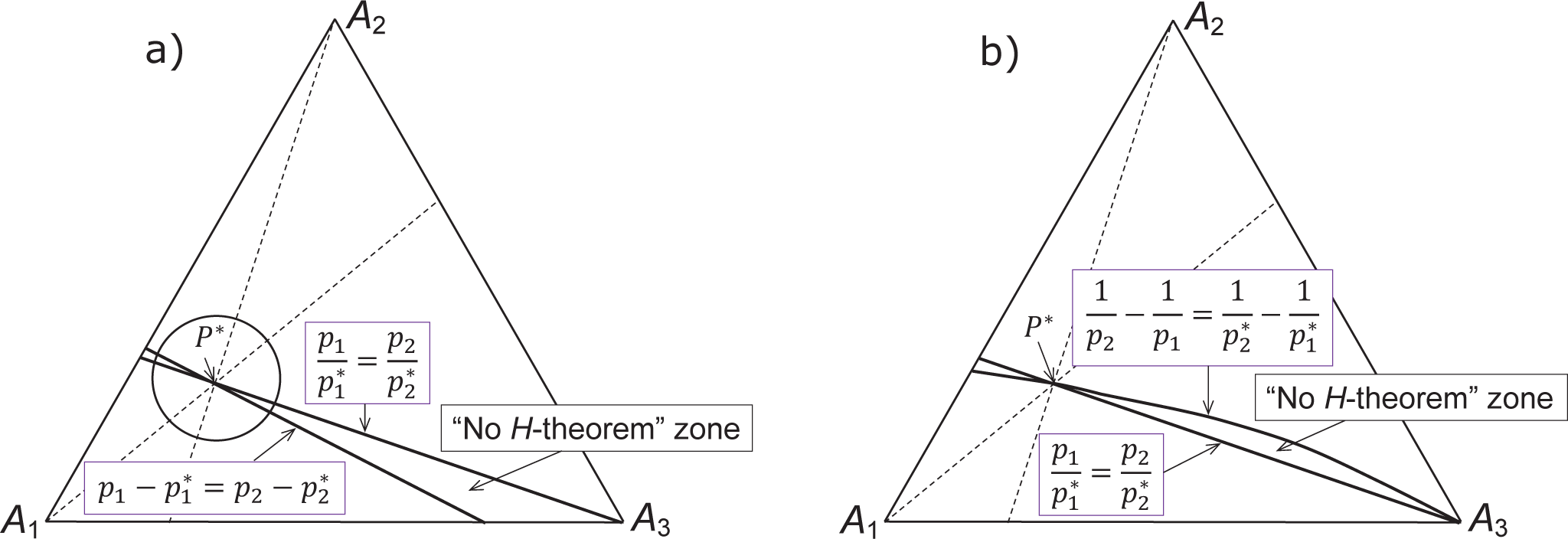
The simplest Bregman divergence is the squared Euclidean distance between P and P*, . The solution to the problem (6) is: . Obviously, it differs from the proportion required by the partial equilibria criterion (Figure 1a).
For the Itakura-Saito distance (2) the solution to the problem (6) is: . It also differs from the proportion required (Figure 1b).
If the single equilibrium in 1D system is not a minimizer of a convex function H then dH/dt > 0 on the interval between the equilibrium and minimizer of H (or minimizers if it is not unique). Therefore, if H(P) does not satisfy the partial equilibria criterion then in the simplex of distributions there exists an area bordered by the partial equilibria surface for Ai ⇌ Aj and by the minimizers for the problem (6), where for some master equations dH/dt > 0 (Figure 1). In particular, in such an area dH/dt > 0 for the simple system with two mutually reverse transitions, Ai ⇌ Aj, and the same equilibrium.
If H satisfies the partial equilibria criterion, then the minimizers for the problem (6) coincide with the partial equilibria surface for Ai ⇌ Aj, and the “no H-theorem zone” vanishes.
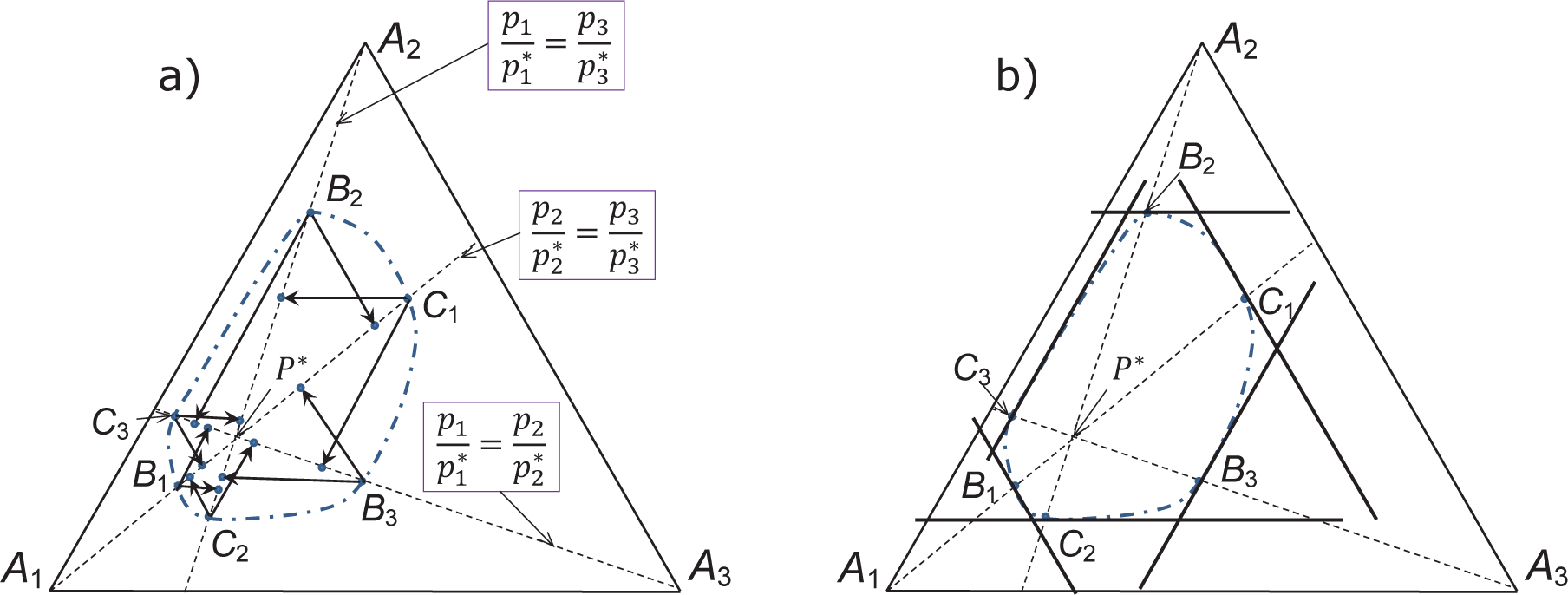
The partial equilibria criterion allows a simple geometric interpretation. Let us consider a sublevel set of H(P) in the simplex ∆n: Uh = {P ∈ ∆n | H(P) ≤ h}. Let the level set be Lh = {P ∈ ∆n | H(P) = h}. For the partial equilibrium Ai ⇌ Aj we use the notation Eij. It is given by the equation . The geometric equivalent of the partial equilibrium condition is: for all i; j (i ≠ j) and every P ∈ Lh ∩ Eij the straight line P + λγij (λ ∈ ℝ) is a supporting line of Uh. This means that this line does not intersect the interior of Uh.
We illustrate this condition on the plane for three states in Figure 2. The level set of H is represented by the dot-dash line. It intersects the lines of partial equilibria (dashed lines) at points B1;2;3 and C1;2;3. For each point P from these six intersections (P = Bi and P = Ci) the line P +λγjk (λ ∈ ℝ) should be a supporting line of the sublevel set (the region bounded by the dot-dash line). Here, i, j, k should all be different numbers. Segments of these lines form a hexagon circumscribed around the level set (Figure 2b).
The points of intersection B1;2;3 and C1;2;3 cannot be selected arbitrarily on the lines of partial equilibria. First of all, they should be the vertices of a convex hexagon with the equilibrium P* inside. Secondly, due to the partial equilibria criterion, the intersections of the straight line P + λγij with the partial equilibria Eij are the conditional minimizers of H on this line, and therefore should belong to the sublevel set UH(P). If we apply this statement to P = Bi and P = Ci, then we will get two projections of this point onto partial equilibria Eij parallel to γij (Figure 2a). These projections should belong to the hexagon with the vertices B1;2;3 and C1;2;3. They produce a six-ray star that should be inscribed into the level set.
In Figure 2 we present the following characterization of the level set of a Lyapunov function for the Markov chains with three states. This convex set should be circumscribed around the six-ray star (Figure 2a) and inscribed in the hexagon of the supporting lines (Figure 2b).
All the f-divergences given by Equation (1) satisfy the partial equilibria criterion and are the universal Lyapunov functions but the reverse is not true: the class of universal Lyapunov functions is much wider than the set of the f-divergences. Let us consider the set “PEC” of convex functions H(P∥P*), which satisfy the partial equilibria criterion. It is closed with respect to the following operations
Conic combination: if Hj(P∥P*) ∈ PEC then for nonnegative coefficients αj ≥ 0.
Convex monotonic transformation of scale: if H(P∥P*) ∈ PEC then F(H(P∥P*)) ∈ PEC for any convex monotonically increasing function of one variable F.
Using these operations we can construct new universal Lyapunov functions from a given set. For example,
is a universal Lyapunov function that does not have the f-divergence form because the first sum is an f-divergence given by Equation (1) with and the product is the exponent of this f-divergence (exp is convex and monotonically increasing function).
The following function satisfies the partial equilibria criterion for every ε > 0.
It is convex for 0 < ε < 1. (Just apply the Gershgorin theorem [28] to the Hessian and use that all .) Therefore, it is a universal Lyapunov function for master equation in ∆n if 0 < ε < 1. The partial equilibria criterion together with the convexity condition allows us to construct many such examples.
5. General H-Theorem for Nonlinear Kinetics
5.1. Generalized Mass Action Law
Several formalisms are developed in chemical kinetics and non-equilibrium thermodynamics for the construction of general kinetic equations with a given “thermodynamic Lyapunov functional”. The motivation of this approach “from thermodynamics to kinetics” is simple [29,30]: (i) the thermodynamic data are usually more reliable than data about kinetics and we know the thermodynamic functions better than the details of kinetic equations, and (ii) positivity of entropy production is a fundamental law and we prefer to respect it “from scratch”, by the structure of kinetic equations.
GMAL is a method for the construction of dissipative kinetic equations for a given thermodynamic potential H. Other general thermodynamic approaches [31–33] give similar results for a given stoichiometric algebra. Below we introduce GMAL following [29,30,34].
The list of components is a finite set of symbols A1, …, An.
A reaction mechanism is a finite set of the stoichiometric equations of elementary reactions:
where ρ = 1, …, m is the reaction number and the stoichiometric coefficients αρi, βρi are nonnegative numbers. Usually, these numbers are assumed to be integer but in some applications the construction should be more flexible and admit real nonnegative values. Let αρ, βρ be the vectors with coordinates αρi, βρi correspondingly.
A stoichiometric vector γρ of the reaction in Equation (18) is a n-dimensional vector γρ= βρ – αρ with coordinates
that is, “gain minus loss” in the ρth elementary reaction. We assume αρ ≠ βρ to avoid trivial reactions with zero γρ.
One of the standard assumptions is existence of a strictly positive stoichiometric conservation law, a vector b = (bi), bi > 0 such that for all ρ. This may be the conservation of mass, of the total probability, or of the total number of atoms, for example.
A nonnegative extensive variable Ni, the amount of Ai, corresponds to each component. We call the vector N with coordinates Ni “the composition vector”. The concentration of Ai is an intensive variable ci = Ni/V, where V > 0 is the volume. The vector c = N/V with coordinates ci is the vector of concentrations.
Let us consider a domain U in n-dimensional real vector space E with coordinates N1, …, Nn. For each Ni, a dimensionless entropy (or free entropy, for example, Massieu, Planck, or Massieu-Planck potential that corresponds to the selected conditions [4]) S(N) is defined in U. “Dimensionless” means that we use S/R instead of physical S. This choice of units corresponds to the informational entropy (p ln p instead of kBp ln p).
The dual variables, potentials, are defined as the partial derivatives of H = −S:
This definition differs from the chemical potentials [4] by the factor 1/RT. We keep the same sign as for the chemical potentials, and this differs from the standard Legendre transform for S. (It is the Legendre transform for the function H = −S.) The standard condition for the reversibility of the Legendre transform is strong positive definiteness of the Hessian of H.
For each reaction, a nonnegative quantity, reaction rate rρ is defined. We assume that this quantity has the following structure (compare with Equations (4), (7), and (14) in [32] and Equation (4.10) in [33]):
where is the standard inner product. Here and below, exp( , ) is the exponent of the standard inner product. The kinetic factor φρ ≥ is an intensive quantity and the expression exp is the Boltzmann factor of the ρth elementary reaction.
In the standard formalism of chemical kinetics the reaction rates are intensive variables and in kinetic equations for N an additional factor—the volume—appears. For heterogeneous systems, there may be several “volumes” (including interphase surfaces).
A nonnegative extensive variable Ni, the amount of Ai, corresponds to each component. We call the vector N with coordinates Ni “the composition vector”. The concentration of Ai is an intensive variable ci = Ni/V, where V > 0 is the volume. If the system is heterogeneous then there are several “volumes” (volumes, surfaces, etc.), and in each volume there are the composition vector and the vector of concentrations [30,34]. Here we will consider homogeneous systems.
The kinetic equations for a homogeneous system in the absence of external fluxes are
If the volume is not constant then the equations for concentrations include V and have different form (this is typical for combustion reactions, for example).
The classical Mass Action Law gives us an important particular case of GMAL given by Equation (21). Let us take the perfect free entropy
where ci = Ni/V ≥ 0 are concentrations and are the standard equilibrium concentrations.
For the perfect entropy function presented in Equation (23)
and for the GMAL reaction rate function given by (21) we get
The standard assumption for the Mass Action Law in physics and chemistry is that φ and c* are functions of temperature: φρ= φρ(T) and To return to the kinetic constants notation and in particular to first order kinetics in the quasichemical form presented in Equation (13), we should write:
5.2. General Entropy Production Formula
Thus, the following entities are given: the set of components Ai (i = 1, …, n), the set of m elementary reactions presented by stoichiometric equations (18), the thermodynamic Lyapunov function H (N, V, …) [4,30,35], where dots (marks of omission) stand for the quantities that do not change in time under given conditions, for example, temperature for isothermal processes or energy for isolated systems. The GMAL presents the reaction rate rρ in Equation (21) as a product of two factors: the Boltzmann factor and the kinetic factor. Simple algebra gives for the time derivative of H:
An auxiliary function θ(λ) of one variable λ ∈ [0; 1] is convenient for analysis of dS/dt (see [29,34,36]):
With this function, Ḣ defined by Equation (27) has a very simple form:
The auxiliary function θ(λ) allows the following interpretation. Let us introduce the deformed stoichiometric mechanism with the stoichiometric vectors,
which is the initial mechanism when λ=1 the reverted mechanism with interchange of α and β when λ=0 and the trivial mechanism (the left and right hand sides of the stoichiometric equations coincide) when λ=1/2. Let the deformed reaction rate be (the genuine kinetic factor is combined with the deformed Boltzmann factor). Then .
It is easy to check that θ″(λ) ≥ 0 and, therefore, θ(λ) is a convex function.
The inequality
is necessary and sufficient for accordance between kinetics and thermodynamics (decrease of free energy or positivity of entropy production). This inequality is a condition on the kinetic factors. Together with the positivity condition φρ ≥ 0 it defines a convex cone in the space of vectors of kinetic factors φρ (ρ = 1, …, m). There exist two less general and more restrictive sufficient conditions: detailed balance and complex balance (known also as semidetailed or cyclic balance).
5.3. Detailed Balance
The detailed balance condition consists of two assumptions: (i) for each elementary reaction in the mechanism (18) there exists a reverse reaction . Let us join these reactions in pairs
After this joining, the total number of stoichiometric equations decreases. We distinguish the reaction rates and kinetic factors for direct and inverse reactions by the upper plus or minus:
The kinetic equations take the form
The condition of detailed balance in GMAL is simple and elegant:
For the systems with detailed balance we can take and write for the reaction rate:
M. Feinberg called this kinetic law the “Marselin-De Donder” kinetics [37].
Under the detailed balance conditions, the auxiliary function θ(λ) is symmetric with respect to change . Therefore, θ(1) = θ(0) and, because of convexity of θ(λ), the inequality holds: θ′(λ) ≥ 0. Therefore, and kinetic equations obey the second law of thermodynamics.
The explicit formula for has the well known form since Boltzmann proved his H-theorem in 1872:
A convenient equivalent form of is proposed in [38]:
where
is a normalized affinity. In this formula, the kinetic information is collected in the nonnegative factors, the sums of reaction rates . The purely thermodynamic multiplier is positive for non-zero . For small | |, the expression behaves like and for large | | it behaves like the absolute value, | |.
The detailed balance condition reflects “microreversibility”, that is, time-reversibility of the dynamic microscopic description and was first introduced by Boltzmann in 1872 as a consequence of the reversibility of collisions in Newtonian mechanics.
5.4. Complex Balance
The complex balance condition was invented by Boltzmann in 1887 for the Boltzmann equation [39] as an answer to the Lorentz objections [40] against Boltzmann’s proof of the H-theorem. Stueckelberg demonstrated in 1952 that this condition follows from the Markovian microkinetics of fast intermediates if their concentrations are small [41]. Under this asymptotic assumption this condition is just the probability balance condition for the underlying Markov process. (Stueckelberg considered this property as a consequence of “unitarity” in the S-matrix terminology.) It was known as the semidetailed or cyclic balance condition. This condition was rediscovered in the framework of chemical kinetics by Horn and Jackson in 1972 [42] and called the complex balance condition. Now it is used for chemical reaction networks in chemical engineering [43]. Detailed analysis of the backgrounds of the complex balance condition is given in [34].
Formally, the complex balance condition means that θ(1) ≡ θ(0) for all values of . We start from the initial stoichiometric equations (18) without joining the direct and reverse reactions. The equality θ(1) ≡ θ(0) reads
Let us consider the family of vectors {αρ,βρ} (ρ = 1, …, m). Usually, some of these vectors coincide. Assume that there are q different vectors among them. Let y1, …, yq be these vectors. For each j = 1, …, q we take
We can rewrite Equation (39) in the form
The Boltzmann factors are linearly independent functions. Therefore, the natural way to meet these conditions is: for any j = 1, …, q
This is the general complex balance condition. This condition is sufficient for the inequality , because it provides the equality θ(1) = θ(0) and θ(λ) is a convex function.
It is easy to check that for the first order kinetics given by Equation (10) (or Equation (13)) with positive equilibrium, the complex balance condition is just the balance equation (11) and always holds.
5.5. Cyclic Decomposition of the Systems with Complex Balance
The complex balance conditions defined by Equation (42) allow a simple geometric interpretation. Let us introduce the digraph of transformation of complexes. The vertices of this digraph correspond to the formal sums (y, A) (“complexes”), where A is the vector of components, and y ϵ {y1, …, yq} are vectors αρ or βρ from the stoichiometric equations of the elementary reactions (18). The edges of the digraph correspond to the elementary reactions with non-zero kinetic factor.
Let us assign to each edge (αρ, A) → (βρ, A) the auxiliary current-the kinetic factor φρ. For these currents, the complex balance condition presented by Equation (42) is just Kirchhoff’s first rule: the sum of the input currents is equal to the sum of the output currents for each vertex. (We have to stress that these auxiliary currents are not the actual rates of transformations.)
Let us use for the vertices the notation Θj: Θj = (yj, A), (j − 1, …, q) and denote φlj the fluxes for the edge Θj → Θl.
The simple cycle is the digraph , where all the complexes Θil (l = 1, …, k) are different. We say that the simple cycle is normalized if all the corresponding auxiliary fluxes are unit: .
The graph of the transformation of complexes cannot be arbitrary if the system satisfies the complex balance condition [22].
Proposition 3
If the system satisfies the complex balance condition (i.e. Equation (42) holds) then every edge of the digraph of transformation of complexes is included into a simple cycle.
Proof
First of all, let us formulate Kirchhoff’s first rule (42) for subsets: if the digraph of transformation of complexes satisfies Equation (42), then for any set of complexes Ω
where φΦΘ is the positive kinetic factor for the reaction Θ → Φ if it belongs to the reaction mechanism (i.e., the edge Θ → Φ belongs to the digraph of transformations) and φΦΘ = 0 if it does not. Equation (43) is just the result of summation of Equations (42) for all (yj, A) = Θ ∈ Ω.
We say that a state Θj is reachable from a state Θk if k = i or there exists a non-empty chain of transitions with non-zero coefficients that starts at Θk and ends at Θj: Θk → … → Θj. Let Θi↓ be the set of states reachable from Θi. The set Θi↓ has no output edges.
Assume that the edge Θj → Θi is not included in a simple cycle, which means Θj ∉ Θi↓. Therefore, the set Ω = Θi↓ has the input edge (Θj → Θi) but no output edges and cannot satisfy Equation (43). This contradiction proves the proposition. □
This property (every edge is included in a simple cycle) is equivalent to the so-called “weak reversibility” or to the property that every weakly connected component of the digraph is its strong component.
For every graph with the system of fluxes, which obey Kirchhoffs first rule, the cycle decomposition theorem holds. It can be extracted from many books and papers [20,26,44]. Let us recall the notion of extreme ray. A ray with direction vector x ≠ 0 is a set {λx} (λ ≥ 0). A ray l is an extreme ray of a cone Q if for any u ∈ l and any x, y ∈ Q, whenever u = (x + y)/2, we must have x, y ∈ l. If a closed convex cone does not include a whole straight line then it is the convex hull of its extreme rays [45].
Let us consider a digraph Q with vertices Θi, the set of edges E and the system of auxiliary fluxes along the edges φij ≥ 0 ((j, i) ∈ E). The set of all nonnegative functions on E, φ: (j, i) ↦ φij, is a nonnegative orthant . Kirchhoffs first rule (Equation (42)) together with nonnegativity of the kinetic factors define a cone of the systems with complex balance .
Proposition 4 (Cycle decomposition of systems with complex balance)
Every extreme ray of Q has a direction vector that corresponds to a simple normalized cycle where all the complexes Θil (l = 1, …, k) are different, all the corresponding fluxes are unit, , and other fluxes are zeros.
Proof
Let a function ϕ: E → ℝ+ be an extreme ray of Q and suppϕ = {(j, i) ∈ E | ϕij > 0}. Due to Proposition 3 each edge from suppϕ is included in a simple cycle formed by edges from suppϕ. Let us take one this cycle . Denote the fluxes of the corresponding simple normalized cycle by ψ. It is a function on E: and ψij = 0 if (i,j) ∈ E but (i,j) ≠ (ij+1,ij) and (i,j) = (i1, ik) (i, j = 1, …, k, i ≠ j).
Assume that suppϕ includes at least one edge that does not belong to the cycle . Then, for sufficiently small κ > 0, ϕ ± κψ ∈ Q and the vector ϕ ± κψ is not proportional to ϕ. This contradiction proves the proposition. □
This decomposition theorem explains why the complex balance condition was often called the “cyclic balance condition”.
5.6. Local Equivalence of Systems with Detailed and Complex Balance
The class of systems with detailed balance is the proper subset of the class of systems with complex balance. A simple (irreversible) cycle of the length k > 2 gives a simplest and famous example of the complex balance system without detailed balance condition.
For Markov chains, the complex balance systems are all the systems that have a positive equilibrium distribution presented by Equation (11), whereas the systems with detailed balance form the proper subclass of the Markov chains, the so-called reversible chains.
In nonlinear kinetics, the systems with complex balance provide the natural generalization of the Markov processes. They deserve the term “nonlinear Markov processes”, though it is occupied by a much wider notion [46]. The systems with detailed balance form the proper subset of this class.
Nevertheless, in some special sense the classes of systems with detailed balance and with the complex balance are equivalent. Let us consider a thermodynamic state given by the vector of potentials defined by Equation (20). Let all the reactions in the reaction mechanism be reversible (i.e., for every transition Θi → Θj the reverse transition Θi ← Θj is allowed and the corresponding edge belongs to the digraph of complex transformations). Calculate the right hand side of the kinetic equations (34) with the detailed balance condition given by Equation (35) for a given value of and all possible values of . The set of these values of Ṅ is a convex cone. Denote this cone QDB( ). For the same transition graph, calculate the right hand side of the kinetic equation (22) under the complex balance condition (42). The set of these values of Ṅ is also a convex cone. Denote it QCB( ). It is obvious that Q DB( ) ⊆ QCB( ). Surprisingly, these cones coincide. In [26] we proved this fact on the basis of the Michaelis-Menten-Stueckelberg theorem [34] about connection of the macroscopic GMAL kinetics and the complex balance condition with the Markov microscopic description and under some asymptotic assumptions. Below a direct proof is presented.
Theorem 2 (Local equivalence of detailed and complex balance)
Proof
Because of the cycle decomposition (Proposition 4) it is sufficient to prove this theorem for simple normalized cycles. Let us use induction on the cycle length k. For k = 2 the transition graph is Θ1 ⇌ Θ2 and the detailed balance condition (35) coincides with the complex balance condition (42). Assume that for the cycles of the length below k the theorem is proved. Consider a normalized simple cycle Θ1 → Θ2 → … Θk → Θ1, Θi = (yi, A). The corresponding kinetic equations are
At the equilibrium, all systems with detailed balance or with complex balance give Ṅ = 0. Assume that the state is non-equilibrium and therefore not all the Boltzmann factors exp( , yi) are equal. Select i such that the Boltzmann factor exp( , yi) has minimal value, while for the next position in the cycle this factor becomes bigger. We can use a cyclic permutation and assume that the factor exp( , y1) is the minimal one and exp( , y2) > exp( , y1).
Let us find a kinetic factor φ such that the reaction system consisting of two cycles, a cycle of the length 2 with detailed balance (here the kinetic factors are shown above and below the arrows) and a simple normalized cycle of the length k − 1, Θ2 → … Θk → Θ2, gives the same Ṅ at the state as the initial scheme. We obtain from Equation (45) the following necessary and sufficient condition (y1 − yk) exp( , yk) + (y2 − y1) exp( , y1) = (y2 − yk) exp( , yk) + φ(y2 − y1)(exp( , y1) − exp( , y2)). It is sufficient to equate here the coefficients at every yi(i = 1, 2, k). The result is
By the induction assumption we proved that theorem for the cycles of arbitrary length and, therefore, it is valid for all reaction schemes with complex balance. □
The cone QDB ( ) of the possible values of Ṅ in Equation (34) is a polyhedral cone with finite set of extreme rays at any non-equilibrium state for the systems with detailed balance. Each of its extreme rays has the direction vector of the form
This follows from the form of the reaction rate presented by Equation (36) for the kinetic equations (34). Following Theorem 2, the cone of the possible values of Ṅ for systems with complex balance has the same set of extreme rays. Each extreme ray corresponds to a single reversible elementary reaction with the detailed balance condition (35).
5.7. General H-Theoremfor GMAL
Consider GMAL kinetics with the given reaction mechanism presented by stoichiometric equations (32) and the detailed balance condition (35). The reaction rates of the elementary reaction for the kinetic equations (34) are proportional to the nonnegative parameter φρ in Equation (36). These m nonnegative numbers φρ (ρ = 1, …, m) are independent in the following sense: for any set of values φρ > 0 the kinetic equations (34) satisfy the H-theorem in the form of Equation (38):
Therefore, nonnegativity is the only a priori restriction on the values ofφρ (ρ = 1, …,m).
One Lyapunov function for the GMAL kinetics with the given reaction mechanism and the detailed balance condition obviously exists. This is the thermodynamic Lyapunov function H used in GMAL construction. For ideal systems (in particular, for master equation) H has the standard form given by Equation (23). Usually, H is assumed to be convex and some singularities (like c ln c) near zeros of c may be required for positivity preservation in kinetics (Ṅi > 0 if ci = 0). The choice of the thermodynamic Lyapunov function for GMAL construction is wide. We consider kinetic equations in a compact convex set U and assume H to be convex and continuous in U and differentiable in the relative interior of U with derivatives continued by continuity to U.
Assume that we select the thermodynamic Lyapunov function H and the reaction mechanism in the form (32). Are there other universal Lyapunov functions for GMAL kinetics with detailed balance and given mechanism? “Universal” here means “independent of the choice of the nonnegative kinetic factors”.
For a given reaction mechanism we introduce the partial equilibria criterion by analogy to Definition 1. Roughly speaking, a convex function F satisfies this criterion if its conditional minima correctly describe the partial equilibria of elementary reactions.
For each elementary reaction from the reaction mechanism given by the stoichiometric equations (32) and any X ∈ U we define an interval of a straight line
Definition 2 (Partial equilibria criterion for GMAL). A convex function F(N) on U satisfies the partial equilibria criterion with a given thermodynamic Lyapunov function H and reversible reaction mechanism given by stoichiometric equations (32) if
for all X ∈ U, ρ = 1, …, m.
Theorem 3
A convex function F(N) on U is a Lyapunov function for all kinetic equations (34) with the given thermodynamic Lyapunov function H and reaction rates presented by Equation (36) (detailed balance) if and only if it satisfies the partial equilibria criterion (Definition 2).
Proof
The partial equilibria criterion is necessary because F(N) should be a Lyapunov function for a reaction mechanism that consists of any single reversible reaction from the reaction mechanism (32). It is also sufficient because for the whole reaction mechanism the kinetic equations (34) are the conic combinations of the kinetic equations for single reversible reactions from the reaction mechanism (32). □
For the general reaction systems with complex balance we can use the theorem about local equivalence (Theorem 2). Consider a GMAL reaction system with the mechanism (18) and the complex balance condition.
Theorem 4
A convex function F(N) on U is a Lyapunov function for all kinetic equations (22) with the given thermodynamic Lyapunov function H and the complex balance condition (42) if it satisfies the partial equilibria criterion (Definition 2).
Proof
The theorem follows immediately from Theorem 3 about Lyapunov functions for systems with detailed balance and the theorem about local equivalence between systems with local and complex balance (Theorem 2). □
The general H-theorems for GMAL is similar to Theorem 1 for Markov chains. Nevertheless, many non-classical universal Lyapunov functions are known for master equations, for example, the f-divergences given by Equation (1), while for a nonlinear reaction mechanism it is difficult to present a single example different from the thermodynamic Lyapunov function or its monotonic transformations. The following family of example generalizes Equation (17).
where f(N) is a non-negative differentiable function and ε > 0 is a sufficiently small number. This function satisfies the conditional equilibria criterion. For continuous H(N) on compact U with the spectrum of the Hessian uniformly separated from zero, this F(N) is convex for sufficiently small ε > 0.
6. Generalization: Weakened Convexity Condition, Directional Convexity and Quasiconvexity
In all versions of the general H-theorems we use convexity of the Lyapunov functions. Strong convexity of the thermodynamic Lyapunov functions H (or even positive definiteness of its Hessian) is needed, indeed, to provide reversibility of the Legendre transform N ↔ ∇H.
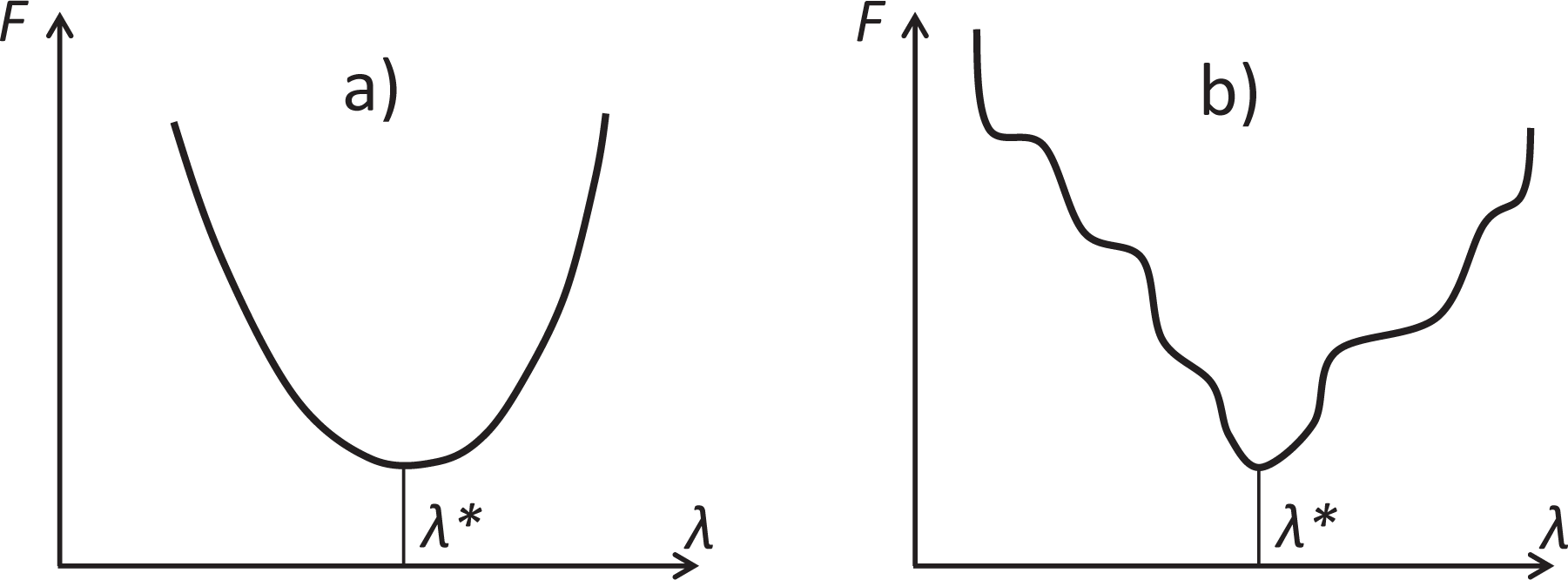
For the kinetic Lyapunov functions that satisfy the partial equilibria criterion, we use, actually, a rather weak consequence of convexity in restrictions on the straight lines X + λγ (where λ ∈ ℝ is a coordinate on the real line, γ is a stoichiometric vector of an elementary reaction): if then on the half-lines (rays) λ ≥ λ* and λ ≤ λ* function F(X + λγ) is monotonic. It does not decrease for λ ≥ λ* and does not increase for λ ≤ λ*. Of course, convexity is sufficient (Figure 3a) but a much weaker property is needed (Figure 3b).
A function F on a convex set U is quasiconvex [47] if all its sublevel sets are convex. It means that for every X, Y ∈ U
In particular, a function F on a segment is quasiconvex if all its sublevel sets are segments.
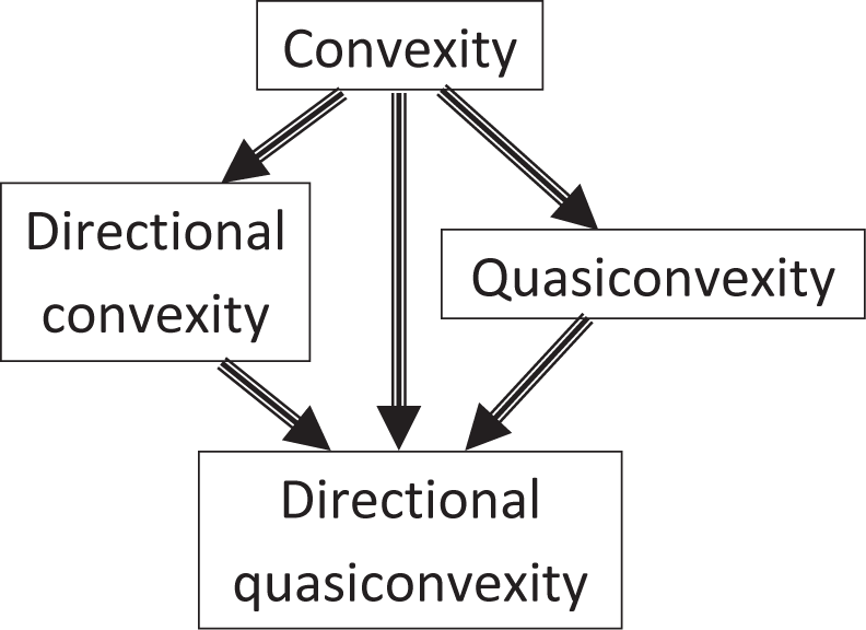
Among many other types of convexity and quasiconvexity (see, for example [48]) two are important for the general H-theorem. We do not need convexity of functions along all straight lines in U. It is sufficient that the function is convex on the straight lines X + ℝ γρ, where γρ are the stoichiometric (direction) vectors of the elementary reactions.
Let D be a set of vectors. A function F is D-convex if its restriction to each line parallel to a nonzero v ∈D is convex [49]. In our case, D is the set of stoichiometric vectors of the transitions, D = {γρ|ρ= 1, …,m}. Wecan use this directional convexity instead of convexity in Propositions 1,2 and Theorems 1,3, 4.
Finally, we can relax the convexity conditions even more and postulate directional quasiconvexity [50] for the set of directions D = {γρ | ρ = 1, …, m}. Propositions 1, 2 and Theorems 1,3,4 will be still true if the functions are continuous, quasiconvex in restrictions on all lines X + R γρ and satisfy the partial equilibria criterion.
Relations between these types of convexity are schematically illustrated in Figure 4.
7. Discussion
Many non-classical entropies are invented and applied to various problems in physics and data analysis. In this paper, the general necessary and sufficient criterion for the existence of H-theorem is proved. It has a simple and physically transparent form: the convex divergence (relative entropy) should properly describe the partial equilibria for transitions Ai ⇌ Aj. It is straightforward to check this partial equilibria criterion. The applicability of this criterion does not depend on the detailed balance condition and it is valid both for the class of the systems with detailed balance and for the general first order kinetics without this assumption.
If an entropy has no H-theorem (that is, it violates the second law and the data processing lemma) then there should be unprecedentedly strong reasons for its use. Without such strong reasons we cannot employ it. Now, I cannot find an example of sufficiently strong reasons but people use these entropies in data analysis and we have to presume that they may have some hidden reasons and that these reasons may be sufficiently strong. We demonstrate that this problem arises even for such popular divergences like Euclidean distance or Itakura-Saito distance.
The general H-theorem is simply a reduction of a dynamical question (Lyapunov functionals) to a static one (partial equilibria). It is not surprising that it can be also proved for nonlinear Generalized Mass Action Law kinetics. Here kinetic systems with complex balance play the role of the general Markov chains, whereas the systems with detailed balance correspond to the reversible Markov chains. The requirement of convexity of Lyapunov functions can be relaxed to the directional convexity (in the directions of reactions) or even directional quasiconvexity.
For the reversible Markov chains presented by Equations (15) with the classical entropy production Formula (16), every universal Lyapunov function H should satisfy inequalities
These inequalities are closely related to another generalization of convexity, the Schur convexity [51]. They turn into the definition of the Schur convexity when equilibrium is the equidistribution with p* 1/n for all i. Universal Lyapunov functions for nonlinear kinetics give one more generalization of the Schur convexity.
Introduction of many non-classical entropies leads to the “uncertainty of uncertainty” phenomenon: we measure uncertainty by entropy but we have uncertainty in the entropy choice [27]. The selection of the appropriate entropy and introduction of new entropies are essentially connected with the class of kinetics. H-theorems in physics are formalizations of the second law of thermodynamics: entropy of isolated systems should increase in relaxation to equilibrium. If we know the class of kinetic equations (for example, the Markov kinetics given by master equations) then the H theorem states that it is possible to use this entropy with the given kinetics. If we know the entropy and are looking for kinetic equations then such a statement turns into the thermodynamic restriction on the thermodynamically admissible kinetic equations. For information processing, the class of kinetic equations describes possible manipulations with data. In this case, the H-theorems mean that under given class of manipulation the information does not increase.
It is not possible to compare different entropies without any relation to kinetics. It is useful to specify the class of kinetic equations, for which they are the Lyapunov functionals. For the GMAL equations, we can introduce the dynamic equivalence between divergences (free entropies or conditional entropies). Two functionals H(N) and F(N) in a convex set U are dynamically consistent with respect to the set of stoichiometric vectors {γρ} (ρ = 1; …; m) if
- (1)
F and H are directionally quasiconvex functions in directions {γρ} (ρ = 1, … m)
- (2)
For all ρ = 1; …; m and N ∈ U
For the Markov kinetics, the partial equilibria criterion is sufficient for a convex function H(P) to be dynamically consistent with the relative entropy Σ i pi(ln(pi=p_ i)1) in the unit simplexΔn. For GMAL, any convex function H(N) defines a class of kinetic equations. Every reaction mechanism defines a family of kinetic equations from this class and a class of Lyapunov functions F, which are dynamically consistent with H. The main message of this paper is that it is necessary to discuss the choice of the non-classical entropies in the context of kinetic equations.
Conflicts of Interest
The author declares no conflict of interest.
References
- Rényi, A. On measures of entropy and information, Proceedings of the 4th Berkeley Symposium on Mathematics, Statistics and Probability, Berkeley, CA, USA, 1960; University of California Press: Berkeley, CA, USA, 1961; 1, pp. 547–561.
- Csiszár, I. Eine informationstheoretische Ungleichung und ihre Anwendung auf den Beweis der Ergodizit¨at von Markoffschen Ketten. Magyar. Tud. Akad. Mat. Kutato Int. Kozl 1963, 8, 85–108. (in German). [Google Scholar]
- Morimoto, T. Markov processes and the H-theorem. J. Phys. Soc. Jap 1963, 12, 328–331. [Google Scholar]
- Callen, H.B. Thermodynamics and an Introduction to Themostatistics, 2nd ed.; Wiley: New York, NY, USA, 1985. [Google Scholar]
- Burg, J.P. The relationship between maximum entropy spectra and maximum likelihood spectra. Geophysics 1972, 37, 375–376. [Google Scholar]
- Cressie, N.; Read, T. Multinomial Goodness of Fit Tests. J. R. Stat. Soc. Ser. B 1984, 46, 440–464. [Google Scholar]
- Tsallis, C. Possible generalization of Boltzmann-Gibbs statistics. J. Stat. Phys 1988, 52, 479–487. [Google Scholar]
- Abe, S., Okamoto, Y., Eds.; Nonextensive Statistical Mechanics and its Applications; Springer: Heidelberg, Germany, 2001.
- Cichocki, A.; Amari, S.-I. Families of alpha- beta- and gamma- divergences: Flexible and robust measures of similarities. Entropy 2010, 12, 1532–1568. [Google Scholar]
- Esteban, M.D.; Morales, D. A summary of entropy statistics. Kybernetica 1995, 31, 337–346. [Google Scholar]
- Gorban, A.N.; Gorban, P.A.; Judge, G. Entropy: The Markov ordering approach. Entropy 2010, 12, 1145–1193, arXiv:1003.1377 [physics.data-an]. [Google Scholar]
- Bregman, L.M. The relaxation method of finding the common points of convex sets and its application to the solution of problems in convex programming. USSR Comput. Math. Math. Phys 1967, 7, 200–217. [Google Scholar]
- Banerjee, A.; Merugu, S.; Dhillon, I.S.; Ghosh, J. Clustering with Bregman divergences. J. Mach. Learn. Res 2005, 6, 1705–1749. [Google Scholar]
- Csiszár, I.; Matúš, F. Generalized minimizers of convex integral functionals, Bregman distance, Pythagorean identities, 2012. arXiv:1202.0666 [math.OC].
- Shannon, C.E. A mathematical theory of communication. Bell Syst. Tech. J 1948, 27, 379. [Google Scholar]
- Cohen, J.E.; Derriennic, Y.; Zbaganu, G.H. Majorization, monotonicity of relative entropy and stochastic matrices. Contemp. Math 1993, 149, 251–259. [Google Scholar]
- Cohen, J.E.; Iwasa, Y.; Rautu, G.; Ruskai, M.B.; Seneta, E.; Zbaganu, G. Relative entropy under mappings by stochastic matrices. Linear Algebra Appl 1993, 179, 211–235. [Google Scholar]
- Gorban, P.A. Monotonically equivalent entropies and solution of additivity equation. Physica A 2003, 328, 380–390. [Google Scholar]
- Amari, S.-I. Divergence, Optimization, Geometry, Proceedings of the 16th International Conference on Neural Information Processing, Bankok, Thailand, 1–5 December 2009; Leung, C.S., Lee, M., Chan, J.H., Eds.; Springer: Berlin, Germany, 2009; pp. 185–193.
- Meyn, S.R. Control Techniques for Complex Networks; Cambridge University Press: Cambridge, UK, 2007. [Google Scholar]
- Meyn, S.R.; Tweedie, R.L. Markov Chains and Stochastic Stability; Cambridge University Press: Cambridge, UK, 2009. [Google Scholar]
- Feinberg, M.; Horn, F.J. Dynamics of open chemical systems and the algebraic structure of the underlying reaction network. Chem. Eng. Sci 1974, 29, 775–787. [Google Scholar]
- Szederkényi, G.; Hangos, K.M.; Tuza, Z. Finding weakly reversible realizations of chemical reaction networks using optimization. Computer 2012, 67, 193–212. [Google Scholar]
- Gorban, A.N. Kinetic path summation, multi-sheeted extension of master equation, and evaluation of ergodicity coefficient. Physica A 2011, 390, 1009–1025. [Google Scholar]
- Van Kampen, N.G. Stochastic processes in physics and chemistry; North-Holland: Amsterdam, The Netherlands, 1981. [Google Scholar]
- Gorban, A.N. Local equivalence of reversible and general Markov kinetics. Physica A 2013, 392, 1111–1121. [Google Scholar]
- Gorban, A.N. Maxallent: Maximizers of all entropies and uncertainty of uncertainty. Comput. Math. Appl 2013, 65, 1438–1456. [Google Scholar]
- Golub, G.H.; van Loan, C.F. Matrix Computations; Johns Hopkins University Press: Baltimore, MD, USA, 1996. [Google Scholar]
- Gorban, A.N. Equilibrium encircling. Equations of Chemical Kinetics and Their Thermodynamic Analysis; Nauka: Moscow, Russia, 1984. (in Russian) [Google Scholar]
- Yablonskii, G.S.; Bykov, V.I.; Gorban, A.N.; Elokhin, V.I. Kinetic Models of Catalytic Reactions; Series Comprehensive Chemical Kinetics; Volume 32, Elsevier: Amsterdam, The Netherlands, 1991. [Google Scholar]
- Grmela, M.; Öttinger, H.C. Dynamics and thermodynamics of complex fluids. I. Development of a general formalism. Phys. Rev. E 1997, 56. [Google Scholar] [CrossRef]
- Grmela, M. Fluctuations in extended mass-action-law dynamics. Physica D 2012, 241, 976–986. [Google Scholar]
- Giovangigli, V.; Matuszewski, L. Supercritical fluid thermodynamics from equations of state. Physica D 2012, 241, 649–670. [Google Scholar]
- Gorban, A.N.; Shahzad, M. The Michaelis-Menten-Stueckelberg Theorem. Entropy 2011, 13, 966–1019. [Google Scholar]
- Hangos, K.M. Engineering model reduction and entropy-based Lyapunov functions in chemical reaction kinetics. Entropy 2010, 12, 772–797. [Google Scholar]
- Orlov, N.N.; Rozonoer, L.I. The macrodynamics of open systems and the variational principle of the local potential. J. Franklin Inst-Eng. Appl. Math 1984, 318, 283–341. [Google Scholar]
- Feinberg, M. On chemical kinetics of a certain class. Arch. Rat. Mechan. Anal 1972, 46, 1–41. [Google Scholar]
- Gorban, A.N.; Mirkes, E.M.; Yablonsky, G.S. Thermodynamics in the limit of irreversible reactions. Physica A 2013, 392, 1318–1335. [Google Scholar]
- Boltzmann, L. Neuer Beweis zweier Sätze über das Wärmegleichgewicht unter mehratomigen Gasmoleküle. Sitzungsberichte der Kaiserlichen Akademie der Wissenschaften in Wien 1887, 95, 153–164. (in German). [Google Scholar]
- Lorentz, H.-A. Über das Gleichgewicht der lebendigen Kraft unter Gasmolekülen. Sitzungsberichte der Kaiserlichen Akademie der Wissenschaften in Wien 1887, 95, 115–152. (in German). [Google Scholar]
- Stueckelberg, E.C.G. Theoreme H et unitarite de S. Helv. Phys. Acta 1952, 25, 577–580. [Google Scholar]
- Horn, F.; Jackson, R. General mass action kinetics. Arch. Ration. Mech. Anal 1972, 47, 81–116. [Google Scholar]
- Szederkényi, G.; Hangos, K.M. Finding complex balanced and detailed balanced realizations of chemical reaction networks. J. Math. Chem 2011, 49, 1163–1179. [Google Scholar]
- Kalpazidou, S.L. Cycle Representations of Markov Processes; Book Series: Applications of Mathematics; Volume 28, Springer: New York, NY, USA, 2006. [Google Scholar]
- Rockafellar, R.T. Convex Analysis; Princeton University Press: Princeton, NJ, USA, 1997. [Google Scholar]
- Kolokoltsov, V.N. Nonlinear Markov Processes and Kinetic Equations; Book series Cambridge Tracts in Mathematics; Volume 182, Cambridge University Press: Cambridge, UK, 2010. [Google Scholar]
- Greenberg, H.J.; Pierskalla, W.P. A review of quasi-convex functions. Oper. Res 1971, 19, 1553–1570. [Google Scholar]
- Ponstein, J. Seven kinds of convexity. SIAM Rev 1967, 9, 115–119. [Google Scholar]
- Matoušek, J. On directional convexity. Discret. Comput. Geom 2001, 25, 389–403. [Google Scholar]
- Hwang, F.K.; Rothblum, U.G. Directional-quasi-convexity, asymmetric Schur-convexity and optimality of consecutive partitions. Math. Oper. Res 1996, 21, 540–554. [Google Scholar]
- Marshall, A.W.; Olkin, I.; Arnold, B.C. Inequalities: Theory of Majorization and its Applications; Springer: New York, NY, USA, 2011. [Google Scholar]


© 2014 by the authors; licensee MDPI, Basel, Switzerland This article is an open access article distributed under the terms and conditions of the Creative Commons Attribution license (http://creativecommons.org/licenses/by/3.0/).
Share and Cite
Gorban, A.N. General H-theorem and Entropies that Violate the Second Law. Entropy 2014, 16, 2408-2432. https://doi.org/10.3390/e16052408
Gorban AN. General H-theorem and Entropies that Violate the Second Law. Entropy. 2014; 16(5):2408-2432. https://doi.org/10.3390/e16052408
Chicago/Turabian StyleGorban, Alexander N. 2014. "General H-theorem and Entropies that Violate the Second Law" Entropy 16, no. 5: 2408-2432. https://doi.org/10.3390/e16052408
APA StyleGorban, A. N. (2014). General H-theorem and Entropies that Violate the Second Law. Entropy, 16(5), 2408-2432. https://doi.org/10.3390/e16052408