Topological Classification of Limit Cycles of Piecewise Smooth Dynamical Systems and Its Associated Non-Standard Bifurcations

Abstract
: In this paper, we propose a novel strategy for the synthesis and the classification of nonsmooth limit cycles and its bifurcations (named Non-Standard Bifurcations or Discontinuity Induced Bifurcations or DIBs) in n-dimensional piecewise-smooth dynamical systems, particularly Continuous PWS and Discontinuous PWS (or Filippov-type PWS) systems. The proposed qualitative approach explicitly includes two main aspects: multiple discontinuity boundaries (DBs) in the phase space and multiple intersections between DBs (or corner manifolds—CMs). Previous classifications of DIBs of limit cycles have been restricted to generic cases with a single DB or a single CM. We use the definition of piecewise topological equivalence in order to synthesize all possibilities of nonsmooth limit cycles. Families, groups and subgroups of cycles are defined depending on smoothness zones and discontinuity boundaries (DB) involved. The synthesized cycles are used to define bifurcation patterns when the system is perturbed with parametric changes. Four families of DIBs of limit cycles are defined depending on the properties of the cycles involved. Well-known and novel bifurcations can be classified using this approach.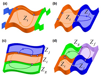
1. Introduction
Piecewise-smooth (PWS) dynamical models have become in valuable tools to analyze many physical systems [1]. Classical qualitative theory based on smooth dynamical systems cannot satisfactorily explain phenomena such as switching and hysteresis in electronic circuits, saturation effects in control systems or friction and impacting behaviors in mechanical systems [2–4]. Therefore, PWS systems of ordinary differential equations are being used to model in a more realistic form these inherent nonsmooth phenomena [5]. The inclusion of PWS functions in dynamical systems has revolutionized qualitative theory and bifurcation theory of dynamical systems [6]. Concepts and methods have had to be formulated or created for nonsmooth cases and many theoretical and practical researches have been developed. However, many open problems remain unsolved [7]. Much work is still needed to achieve a unified and general analytical framework to classify non-standard bifurcations (or Discontinuity Induced Bifurcations – DIBs) in PWS dynamical systems [8]. In this work, we propose a novel strategy for the synthesis and the classification of nonsmooth limit cycles and its bifurcations in n-dimensional PWS dynamical systems, particularly Continuous PWS and Discontinuous PWS (or Filippov-type PWS systems) [9].
The proposed qualitative approach includes two main aspects explicitly: multiple discontinuity boundaries (DBs) in the phase space and multiple intersections between DBs (or corner manifolds— CMs). Figure 1 shows an example of generic non-smooth cycle formed by multiple smooth flows. Previous classifications of DIBs of limit cycles have been restricted to generic cases with a single DB or a single CM [10]. Kuznetsov et al. [11], proposed in 2003 a full catalog of local and global bifurcations in Filippov systems based on classical approach of topological equivalence. Bifurcations of cycles were classified in four main groups: touching bifurcations (when a cycle collides with a boundary of a sliding segment), sliding disconnection bifurcations (when a double tangency appears in a sliding cycle), buckling bifurcations and crossing bifurcations. This classification only considers the simplest possible nonsmooth cycles with a single DB. Sliding cycles can also cross DB and have more than one sliding segment, while crossing cycles can return to DB more than twice.
In other work, di Bernardo et al. [5] classified DIBs in PWS flows in two main groups: grazing bifurcations and sliding bifurcations. A grazing bifurcation occurs when a limit cycle intersects tangentially one of the switching manifolds in phase space [12]. A sliding bifurcation occurs when ever a limit cycle develops an intersection with a sliding region (a region on one of the system switching manifolds where sliding is possible) [1]. Four subgroups of sliding bifurcations were distinguished: sliding–crossing, switching–sliding, grazing—sliding and adding—sliding [8].
Recently, Jeffrey and Hogan [13], have complemented previous classifications of sliding bifurcations using singularity theory of scalar functions. Two types of bifurcations were proposed: regular sliding bifurcations and catastrophic sliding bifurcations. Eight one-parameter sliding bifurcations were characterized, four in each type. This method can be extended to sliding bifurcations of co-dimension two or higher. The main disadvantage of this method is still the comprehensive characterization of bifurcations scenarios with multiple discontinuity boundaries or corner manifolds. Figure 2 shows several examples of PWS state spaces with multiple DBs and CMs.
Physical applications can exhibit multiple DBs or CMs due to nonsmooth phenomena such as friction, saturation or hysteresis. Casini et al. [15] have studied several mechanical systems with multiple DBs caused by the presence of multiple frictional contacts. The model of a non-smooth rotational oscillator in contact with one or two different rough discs rotating with constant driving velocities is considered [15] and the model of double-belt friction oscillator (DBO) is proposed [16]. Both works describe non-standard bifurcations that occur by influence of several DBs. These bifurcations were not characterized completely due to the absence of a framework that allows to finding differences between nonsmooth cycles caused by multiple DBs or CMs. For example, the right side of Figure 2 presents a nonsmooth limit cycle of a mechanical oscillator with double cam [14]. Previous frameworks can not uniquely identify each limit cycle that interact with multiple DBs. In this paper, we propose a novel strategy that allows to classifying limit cycles and bifurcations in PWS dynamical systems with multiple DBs or CMs.
This methodology of synthesis and classification can also be used to characterize complex bifurcation scenarios due to the variation of one or more parameters. First, the PWS state space is modelled using semi-algebraic sets and later, the nonsmooth cycles are synthesized following rules based on piecewise topological equivalence. Families, groups and subgroups of cycles are defined depending on smoothness zones and discontinuity boundaries (DB) involved. Each non smooth cycle is decomposed in smooth segments limited by characteristic points on DB. Crossing, sliding and singular sliding points on DB are determined using the integration-free method named Singular-Point Tracking (SPT) [17,18].
The cycles synthesized are used to define bifurcation patterns when the system is perturbed with parametric changes. Four families of DIBs of limit cycles are defined depending on the properties of the cycles involved. Well-known and novel bifurcations can be classified using this approach.
The paper is organized as follows: in Section 2 is sequencially presented the steps in the arranging of the cycles into orderly categories and with them proceed into the definicion of the systemic grouping of the Non-Standard Bifurcations. In Subsection 2.1 Piecewise Topological Equivalence is presented as the tool to compare cycle structures. In Subsection 2.2 Cycle Stability and Direction are presented as differentiating characteristics. In Subsection 2.3 special points in the orbits of cycles are presented as separating elements of segments formed by points of the same type and also as characterizers that make a topological difference between two cycles. The generalizacion of the Hierarchical Combination of the possible different elements of the cycle is presented in Subsection 2.4. In Subsection 2.5 the nonsmooth limit cycles are used as a methodology to synthesize and classify Discontinuity-Induced Bifurcations (DIBs) of nonsmooth limit cycles in PWS dynamical systems. Section 3 presents the utility of the classification and gives reference papers on the use of the methodology that is developing.
2. Results
Now, we propose a novel strategy to synthesize nonsmooth limit cycles in n-dimensional PWS dynamical systems. Two main aspects are included explicitly: multiple discontinuity boundaries (DBs) in the state space and multiple intersections between DBs (or Corner Manifolds—CMs). The synthesis of nonsmooth limit cycles is based on piecewise topological equivalence.
Let φt and φ̃t represent the evolution operators of two PWS dynamical systems defined by countably many different smooth flows φi(x, t) and φ̃i(x, t) in finitely many phase space regions Zi and respectively, i = 1,..., N. Two such PWS systems are called Piecewise-Topologically Equivalent if [5]:
- (1)
They are topologically equivalent, i.e. there is a homeomorphism h that maps the orbits of the first system onto orbites of the second one, preserving the direction of time so that φt(x) = h−1(φ̃s(h(x))) where the map t → s(t) is continuous and invertible.
- (2)
h can be chosen so that being restricted to the closure, Z̃i, of each region Zii = 1,..., N is also a homeomorphism such that Zi → Z̃i and ∑ij → ∑̃ij
- (3)
Moreover h can be chosen such that for each j, h restricted to Rn/Z̃j and h restricted to Rn/int(Zj) is also a homeomorphism (where int(Zj) is the set of interior points of Zj).
According to the previous definition, two phase portraits can be topologically equivalent but not piecewise-topologically equivalent. Therefore, we can identify all options of nonsmooth limit cycles applying PWS topological equivalence.
Let
 be a limit cycle defined by the topological structure
 = {sta, dir, Fbp, Λ ϑ} where sta contains stability conditions, dir contains flow direction conditions, Fbp is the topological identifier of the cycle, Λ is the topological set array and ϑ is the topological sequence array. The array Λ contains the topological union set(U), the topological point set(Ω) and the topological border set(B). The array ϑ contains the topological union sequenceϑU, the topological point sequenceϑP, and the topological border sequenceϑ∑Γ. Table 1 summarizes the notation used in the synthesis and classification of nonsmooth limit cycles.
Each element of the topological structure
will be explained along this section. Mean while, a limit cycle
characterized by a topological structure
is noted with the sintaxis presented in Equation (1):
Time information such as initial time (t0 = with x(t0) ∈ ∑, switching instants (ti for i = 1,2,..., ω − 1) or period (T = tw − t0) is not included in the topological structure
. Time information is not indispensable in thetopological description of limit cycles. Therefore, two limit cycles
 and
and
 are PWS topologically equivalent if their topological structures
 and
and
 are identical (independent of the time characteristics).
2.1. Stability and Direction of Limit Cycles
Stability and flow direction are very important in the topological structure of a limit cycle. These conditions should be evaluated before other conditions to guarantee topological equivalence. Two limit cycles
and
that are PWS topologically equivalent should have the same conditions of stability and flow direction. Stable cycles, unstable cycles and semi-stable cycles can be distinguished. We also consider two different conditions of flow direction in limit cycles: Clockwise Limit Cycle  and Anticlockwise Limit Cycle
  . In Table 2 we identify four different conditions of stability in limit cycles and annexing the direction the amount is duplicated:
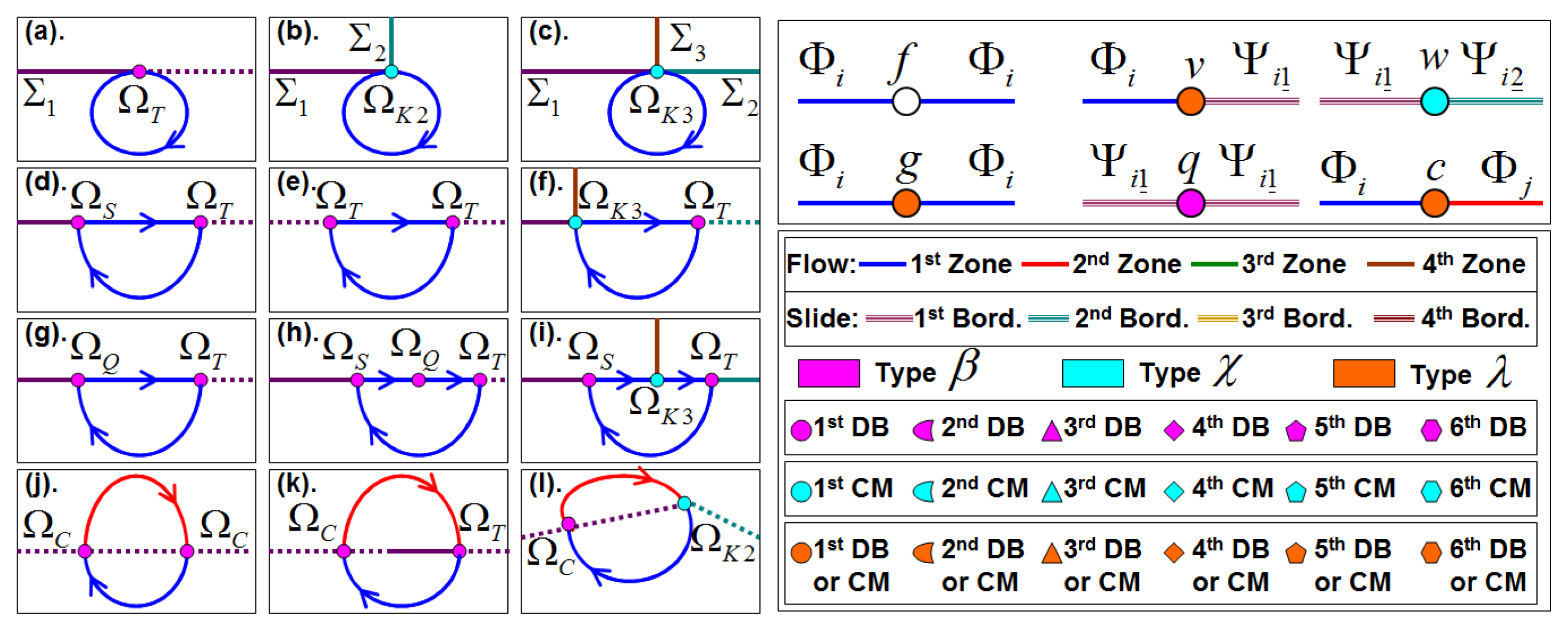
2.3. Characteristic Points of Limit Cycles on DB
In Filippov-type PWS, the periodic solutions or cycles can be divided in standard, sliding or crossing cycles. In the standard cycles, the flow lies entirely in Zi zone. The sliding cycles have sliding stable points on DB and the crossing cycles have crossing or singular sliding points on DB. Each nonsmooth limit cycle can be defined by a composition of flows Φi in the smooth Zi and slide segments ψi_ in the borders (DB or CM). The points where the cycle has a change of flow Φi or slide segments ψi_ is determined by a characteristic point. Therefore, each nonsmooth limit cycle has at least one characteristic point.
A crossing periodic solution can pass through the boundary of the sliding segment. Sliding cycles can cross ∑ and have more than one sliding segment, while crossing cycles can return to ∑ more than twice. Also, corner points can be characteristic points of a nonsmooth limit cycle. Four main types of characteristic points are distinguished:
- (1)
Grazing points (ΩT)
- (2)
Crossing points (ΩC)
- (3)
Sliding end points (singular sliding points (ΩT, or ΩQ), or non singular sliding points (ΩS)) and
- (4)
Corner points (Ωk).
Characteristic points on DB can be identified using the Singular Point Tracking (SPT) method explained in previous works [17–19]. The set of characteristic points in a limit cycle constitutes the topological point set (Ω) while the sequence of characteristic points in a limit cycle constitutes the topological point sequence (ϑP).
The topological structure
should be supplemented with the sets: U (topological union set) and B (topological border set) and with the sequences: ϑU (topological union sequence) and the ϑ∑Γ (topological border sequence). Six types of topological unions can be identified in limit cycles of a PWS system:
- (1)
If the cycle does not have a contact point with a border, then the cycle is known as a standard cycle and a point verifying the periodicity condition can be defined. This point is a union where the flows do not change smooth zone (Φi to Φi) and denominated as type f.
- (2)
If the cycle has a contact point with a border and the flows before and after the contact point do not change of smooth zone (Φi to Φi) then the cycle has a union type g (or grazing).
- (3)
The union is named type c (or crossing) when the flows before and after the characteristic point change of smooth zone (Φi and Φj).
- (4)
The union between a smooth flow and a sliding segment (Φi and ψi_) is noted by type v.
- (5)
A characteristic point between two sliding segments (ψi_ and ψj_) defined by different vector fields is defined by a union type w.
- (6)
While a characteristic point between two sliding segments (ψi_ and ψi_) defined by the same vector fields is known as pseudo-equilibrium point and it is denominated as a union type q.
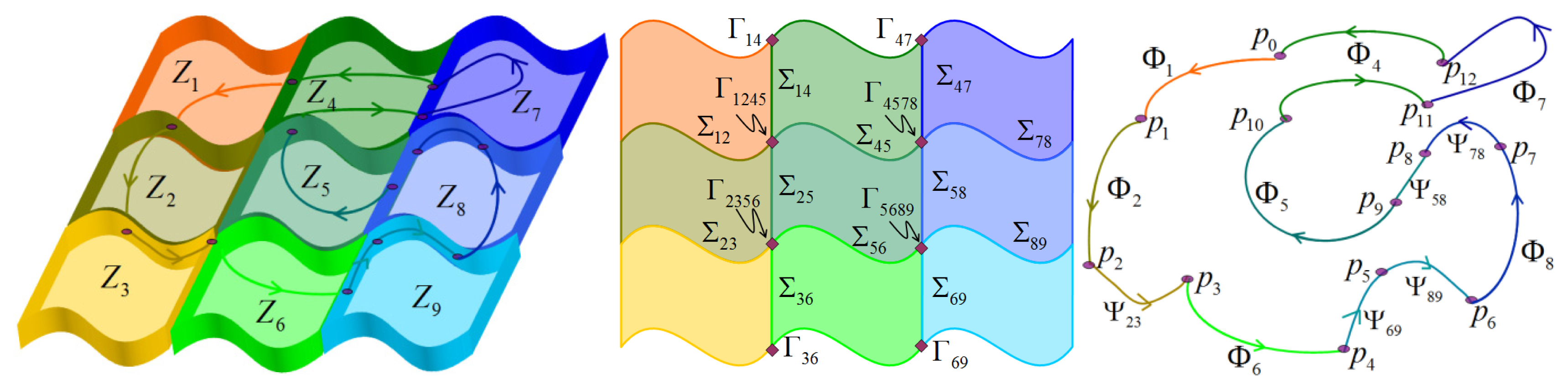
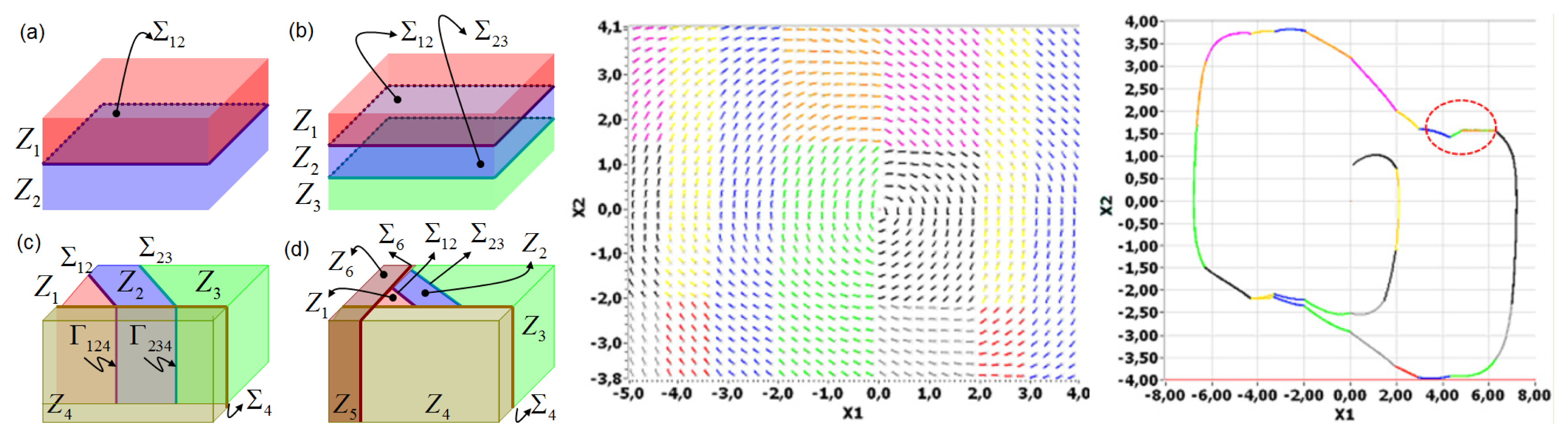
Figure 3 illustrates the six topological unions and their differences. Points defined as union type g, v, or c belong to discontinuity boundaries (DB) or corner manifolds (CM). Points defined as union type q belong to discontinuity boundaries (DB), while points defined as union type w belong to corner manifolds (CM). Therefore, three conditions of borders are considered. Border β when the topological union demands a DB. Border χ when the topological union demands a CM. Border λ when the union does not demand a special border (DB or CM). Also, each zone and border involved in a nonsmooth limit cycle should be labeled with a number (or a color code). For example: first zone (blue), second zone (red), third zone (green) or fourth zone (brown).
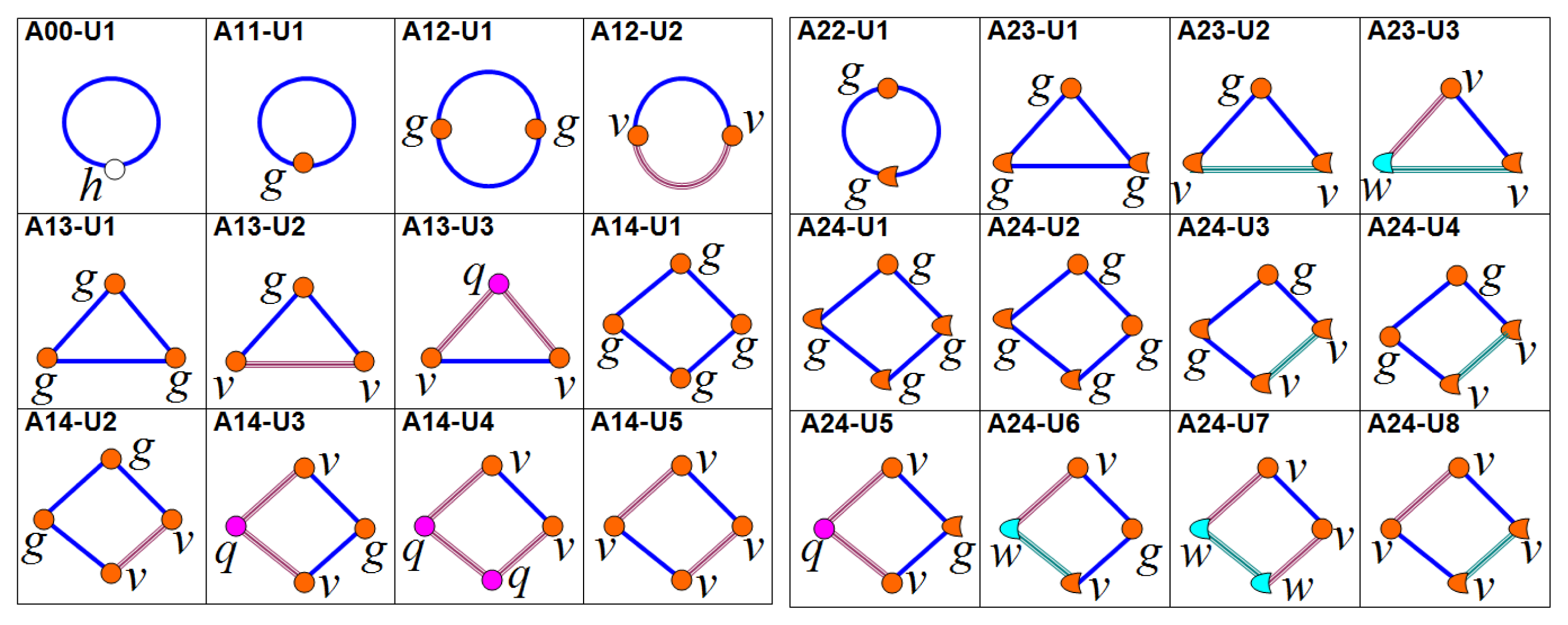
Now, topological graphs can be defined to analyze the connectivity patterns of each nonsmooth limit cycle. Let a topological graph of a nonsmooth limit cycle be a graph for which every vertex corresponds with a characteristic point and every edge corresponds with a smooth flow or a sliding segment. A topological graph synthesizes the topological structure
of a nonsmooth limit cycle. Two PWS topologically equivalent cycles should have the same topological graph. The number of vertexes and edges of atopological graph are important but not exclusive properties of the topological graph. Other properties such as union types and border types should be evaluated to determine PWS Topological equivalence of limit cycles. Therefore, isomorphic topological graphs do not imply that corresponding limit cycles are PWS topologically equivalent. All possible combinations of nonsmooth limit cycles can be easily synthesized by using topological graphs. Figures 4 and 5 show examples of different topological graphs.
Finally, the topological structure
is completely defined when the topological identifier (Fbp) is defined. The topological identifier Fbp of a nonsmooth limit cycle is a label that synthesizes the main features of
. The number of smooth zones involved in the limit cycle, the number of borders involved in the limit cycle and the number of characteristic points in the limit cycle are given by Fbp. The topological identifier Fbp is also fundamental in the proposed classification of limit cycles. In next section, we introduce a methodology to classify nonsmooth limit cycles in piecewise-smooth dynamical systems.
2.4. Hierarchical Classification of Limit Cycles
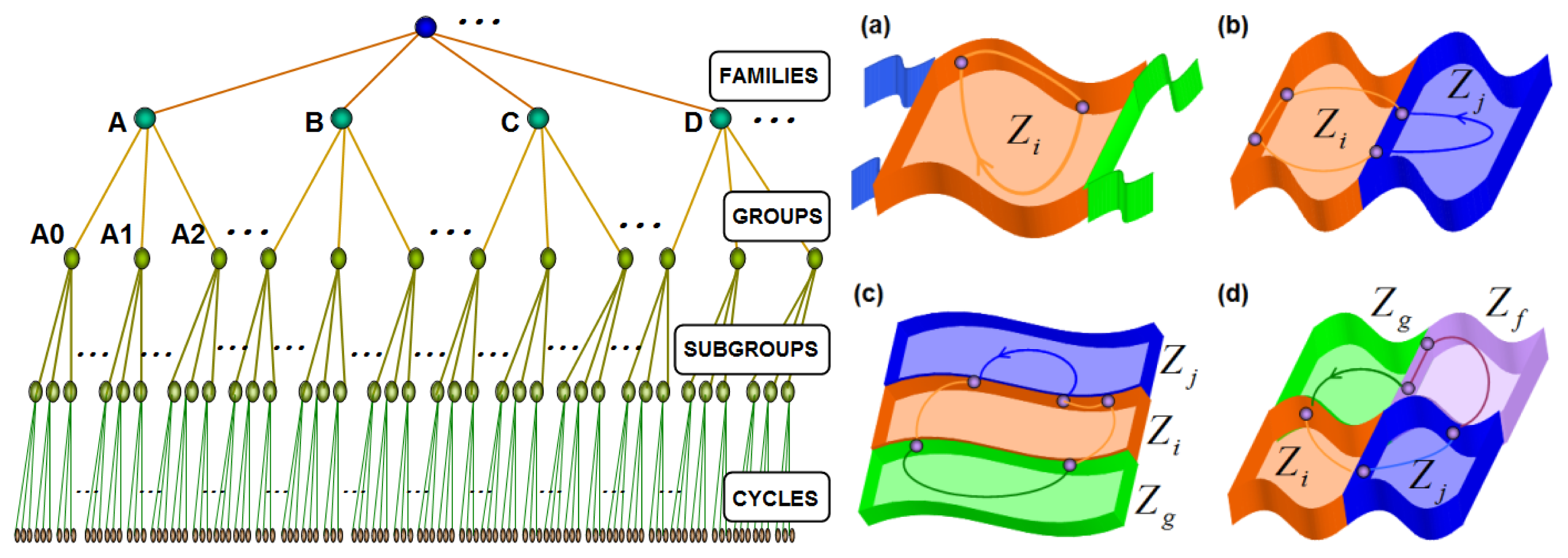
The rules based on the concept of piecewise topological equivalence are used in this section to define a hierarchical classification of nonsmooth limit cycles in PWS dynamical systems. Figure 6 shows the proposed hierarchical structure. Families of cycles, groups of cycles and subgroups of cycles can be defined depending on topological characteristics of nonsmooth limit cycles.
Families of cycles are defined depending on the number of smooth zones involved in the nonsmooth limit cycles. Each family is identified with a capital letter in the following form:
- (1)
Family A contains nonsmooth limit cycles that evolve in one zone and its limits (DB or CM);
- (2)
Family B contains nonsmooth limit cycles that evolve in two zones and their limits (DB or CM);
- (3)
Family C contains nonsmooth limit cycles that evolve in three zones and their limits (DB or CM).
The set of families of nonsmooth limit cycles LC has infinite elements (families) LC = A, B, C, D , E,..., Ā, B̄, C̄, D̄, Ē,..., ..., A̿, B̿, C̿, D̿, ...}.
Groups of cycles can be defined in each family of cycles. Groups of cycles are defined depending on the number of limits (DBs or CMs) involved in the nonsmooth limit cycles. Each group is identified with the capital letter of the family followed by an integer number that represents the quantity of limits involved in the nonsmooth limit cycles. Each family of cycles can contain infinite groups of cycles. For example, family A has the groups: A0, A1, A2, A3, ...; family B has the groups: B1, B2, B3, B4,…; family C has the groups: C2, C3, C4, C5,…; family D has the groups: D3, D4, D5, D6, ...; and so forth. Family B implies at least one border involved in the nonsmooth limit cycles, therefore B0 cannot exist. Also, family C implies at least two borders involved in the nonsmooth limit cycles, therefore C0 and C1 cannot exist.
Subgroups of cycles can be defined in each group of cycles. Subgroups of cycles are defined depending on the number of characteristic points involved in the nonsmooth limit cycles. Each subgroup is identified with the capital letter of the family followed by the number of the group, followed by the number that represents the quantity of characteristic points involved in the nonsmooth limit cycles. The syntaxis of a subgroup identifier coincides with the syntaxis of the topological identifier Fbp of a nonsmooth limit cycle. Each group of cycles can contain finite or infinite subgroups of cycles. For example, group A0 only has one subgroup: A00 that contains all standard cycles; group A1 has the subgroup: A11, A12, A13, A14, ...; group A2 has the subgroup: A22, A23, A24, A25, ...; group A3 has the subgroup: A33, A34, A35, A36, ...; group B1 has the subgroup: A11, B12, B13, B14, B15,...; group C2 has the subgroup: C24, C25, C26, C27,...; and so forth. Group B1 implies at least two characteristic points involved in the nonsmooth limit cycles, therefore B10 and B11 cannot exist. Group C2 implies at least four characteristic points involved in the nonsmooth limit cycles, therefore C20, C21, C22 and C23 cannot exist.
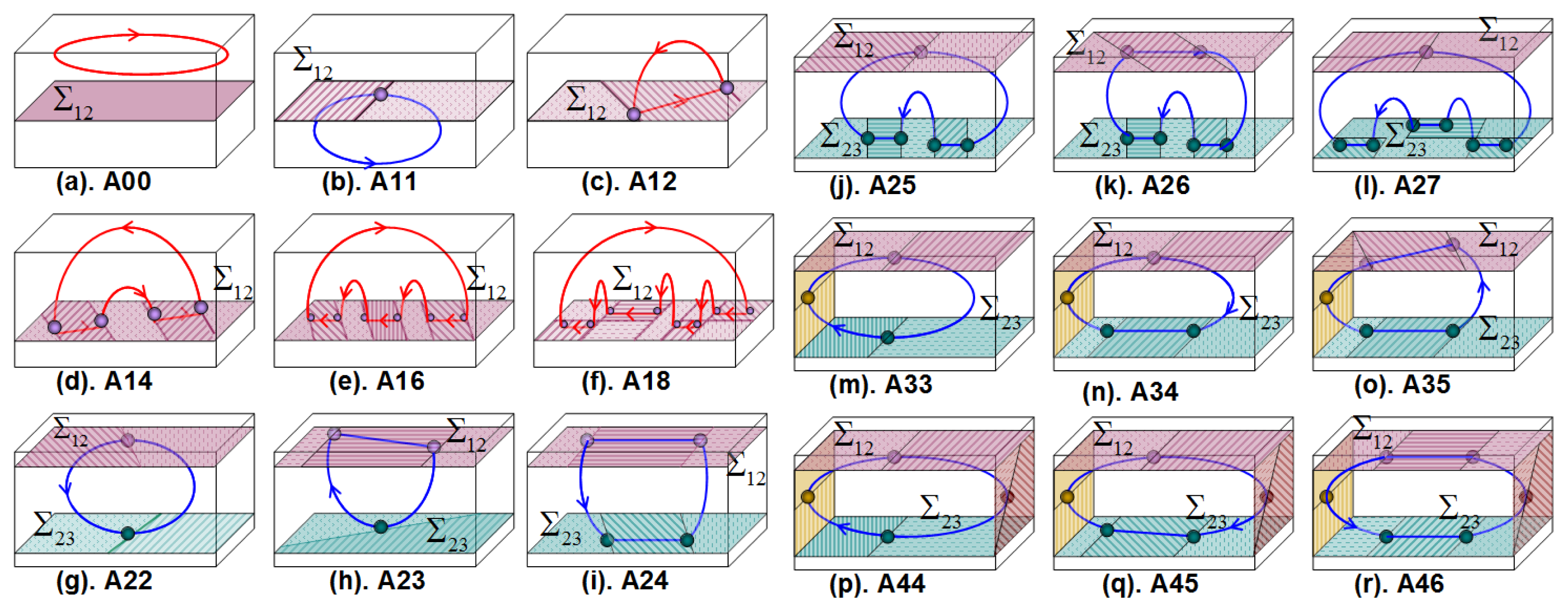
Figure 7 shows examples of nonsmooth limit cycles on Family A in two-dimensional and three-dimensional Filippov-type PWS dynamical systems, respectively. We can identify the topological structure of each limit cycle and its agreement with the topological identifier Fbp. We can assume that all cycles are stable. Clockwise and anticlockwise direction can be distinguished. Also, different number of involved borders and involved characteristic points can be determined.
Revisiting Tables 3 and 4, these summarize the main characteristics of topological graphs presented in Figures 4 and 5, respectively. Different cases can be determined for limit cycles with the same topological identifier Fbp depending on the sequences: ϑU, ϑP and ϑ∑Γ. Topological identifier A00 defines a standard (smooth) cycle while A11 defines a grazing cycle. Sliding cycle and double-grazing cycle (with the same border) have the same topological identifier A12 but different topological unions. Topological union sequences and flow compositions are presented in Table 3 for three A13 cases and five A14 cases. Table 4 shows characteristics of nonsmooth limit cycles of groups A2. Cases with the same topological identifier Fbp and with the same topological union sequence ϑU are distinguished by means of topological border sequence ϑ∑Γ.
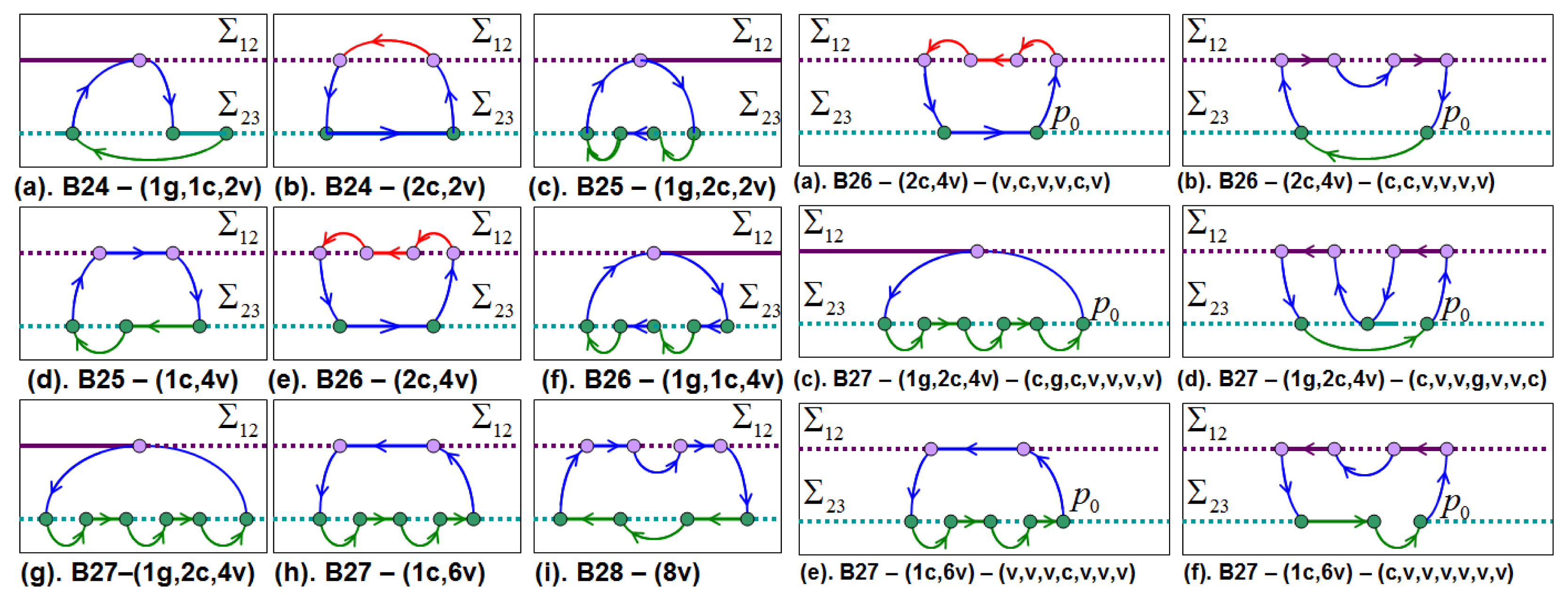
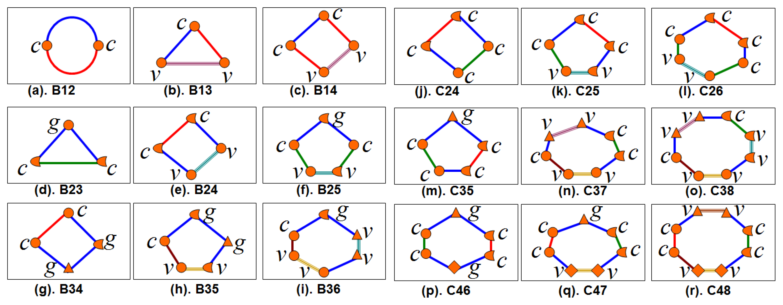
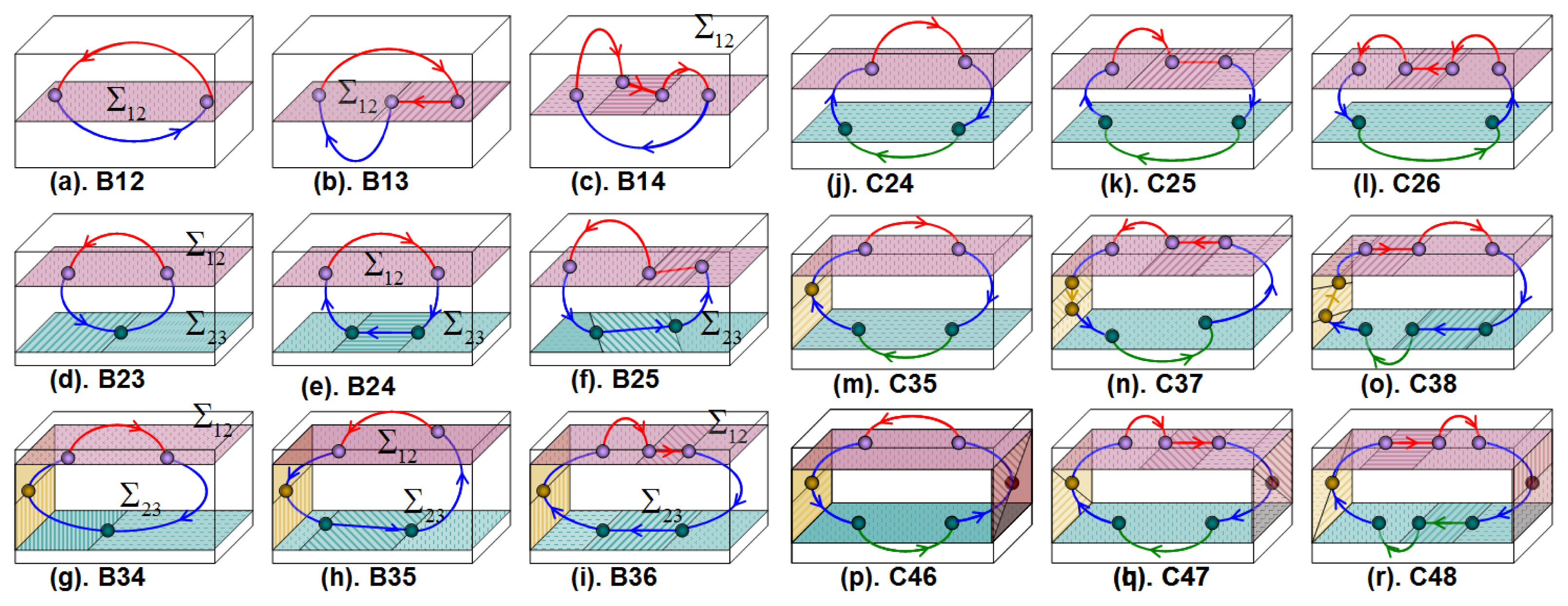
Figure 8 shows examples of nonsmooth limit cycles on Family B and C in three-dimensional Filippov-type PWS dynamical systems. Topological graphs of these cycles were presented in Figure 5. Simplest crossing cycle has the topological identifier B12. Sliding cycles involving two smooth zones have topological identifiers B12, B14, B24, B25, B35 or B36. Non-sliding cycles involving two smooth zones have topological identifiers B23 or B34. Crossing cycle involving three smooth zones has a topological identifier C24. Sliding cycles involving three smooth zones have topological identifiers C25, C26, C37, C38, C47 or C48. Different grazing cycles are shown in Figures 8 and 9 with topological identifiers B23, B25, B34, B35, B36, C35, C46 and C47 where the cycles B35 and C46 are double-grazing cycles (with different borders). A nonsmooth cycle such as the cycle with topological identifier B36 can have combined characteristic of grazing, crossing and sliding cycles. This type of cycles has not been well studied yet.
Figure 9 shows examples of limit cycles of family B with the same topological identifier but different types of topological unions. Multi-sliding and multi-crossing cycles can have the same topological identifier but the types of unions are different. Figure 9 (right) shows examples of limit cycles on family B with the same topological identifier, the same types of topological unions but different topological union sequence. For example, the cycles (a) and (b) have the same topological identifier B26, both cycles with two characteristic points type c and four characteristic points type v. However, the cycle (a) has two sliding segments in different DB while the cycle (b) has two sliding segments in the same DB.
2.5. Synthesis and Classification of DIBs of Limit Cycles
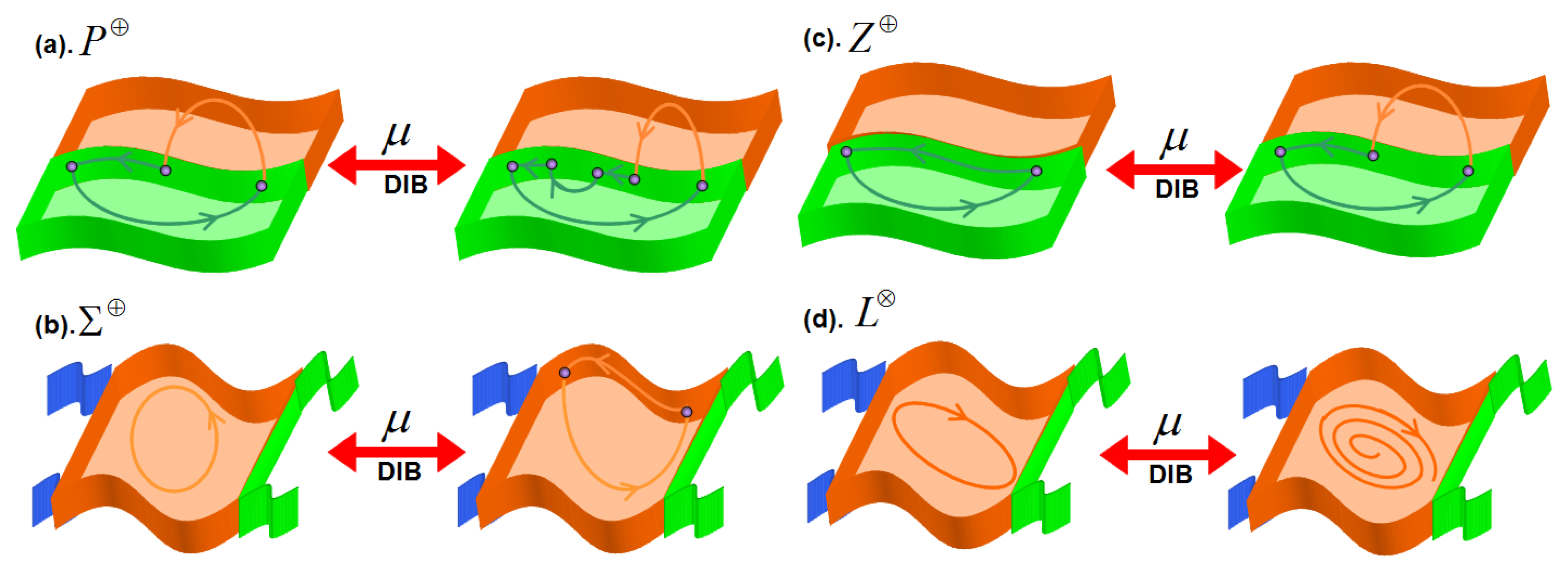
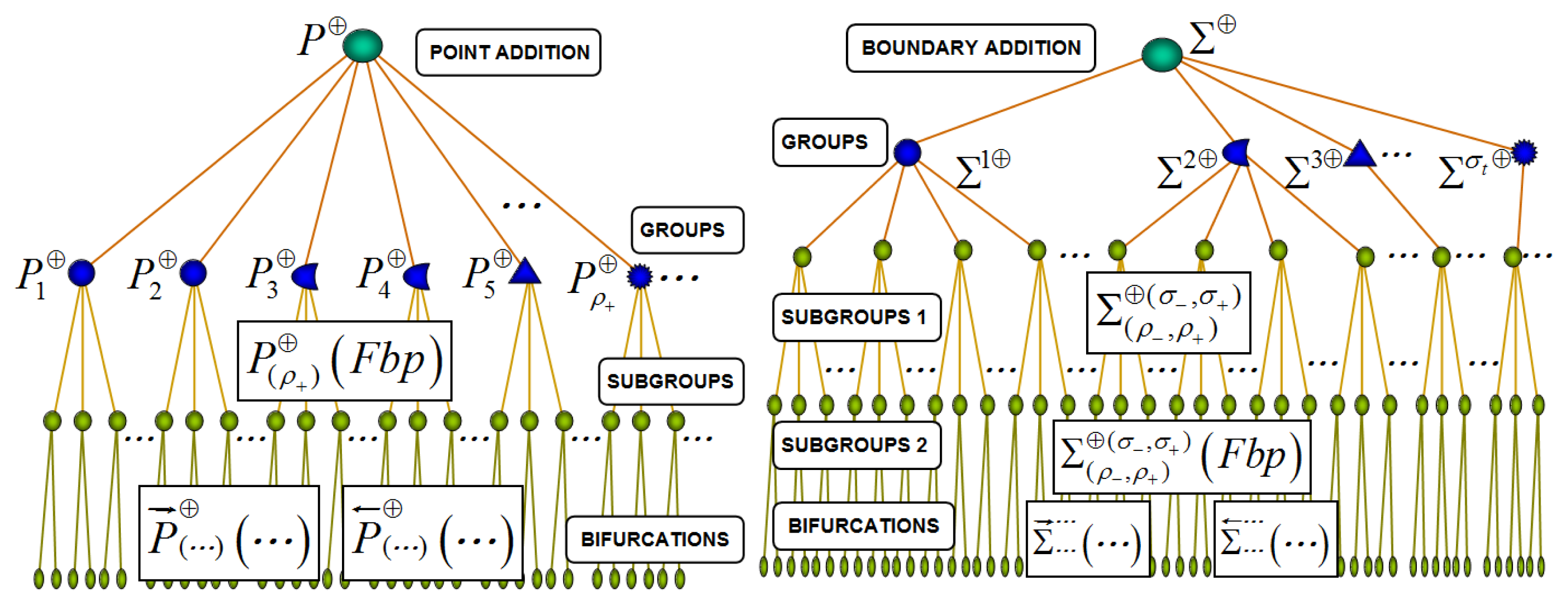
Now, the synthesis and classification of nonsmooth limit cycles are used to propose a novel methodology to synthesize and classify Discontinuity-Induced Bifurcations (DIBs) of nonsmooth limit cycles in PWS dynamical systems. Discontinuity-Induced Bifurcations (DIBs) of nonsmooth limit cycles can be contained in four families of DIBs (NSB):
- (1)
Point Addition DIB Family P⊕,
- (2)
Boundary Addition DIB Family ∑⊕,
- (3)
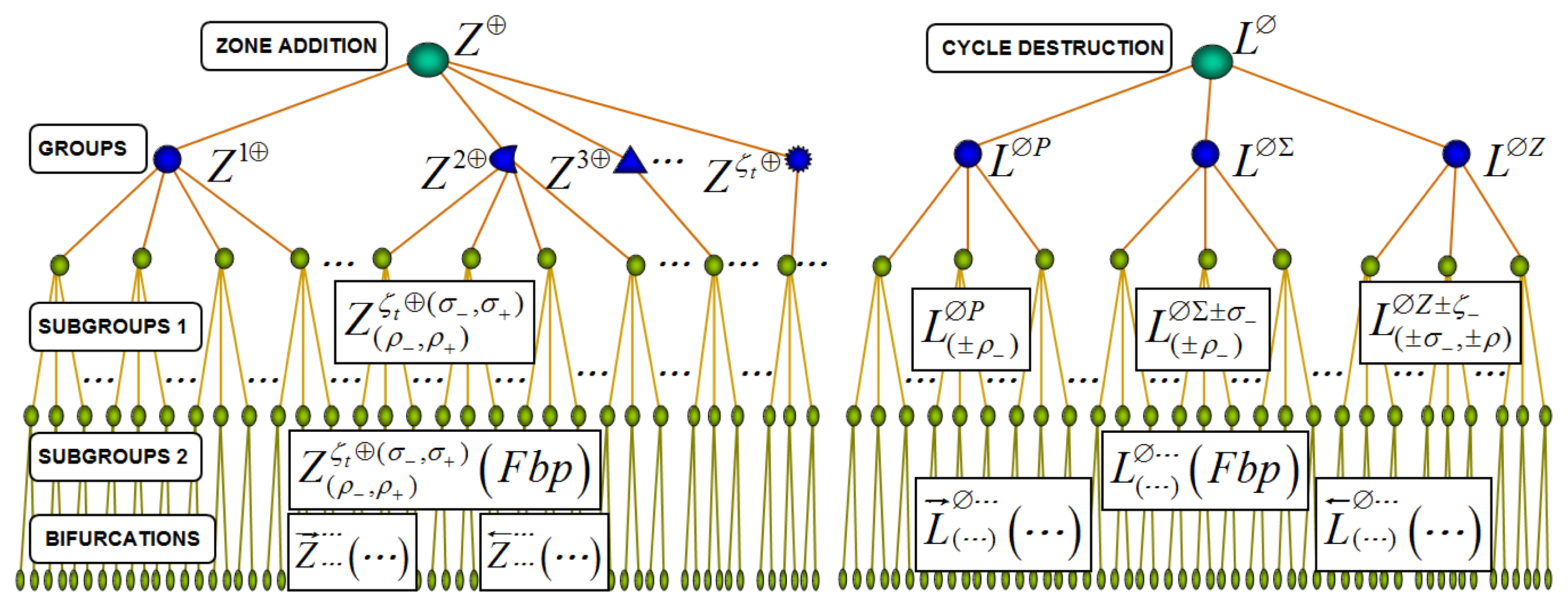
Zone Addition DIB Family Z⊕ and
- (4)
Cycle Destruction DIB Family (L⊗)
Figure 10 shows generic transitions of limit cycles due to variation of a parameter (μ). Table 5 summarizes the notation used in the synthesis and classification of DIBs of limit cycles.
Each family of DIBs (NSB) can be classified in groups of DIBs, subgroups of DIBs and DIBs. Hierarchical structures of each family of DIBs are presented in Figures 11 and 12. Well-known and novel bifurcations can be analyzed with this approach.
Point Addition DIB Family P⊕ contains bifurcations where the nonsmooth limit cycles change of subgroups of limit cycles when the parameter is varied. The number of zones involved in the limit cycles and the number of borders involved in the limit cycles before and after the DIB do not change. Nonsmooth limit cycles before the DIB have the same topological identifier Fbp than the cycle in the critic value. A cycle after the DIB has ρ additional points on DB than the cycle in the critic value. Table 6 presents examples of DIBs that belong to bifurcation family P⊕. The topological identifier and topological union sequence after the DIB are different.
Boundary Addition DIB Family (∑⊕) contains bifurcations where the number of borders involved in the nonsmooth limit cycles changes due to variation of a parameter (σ−, σ+). The number of zones involved in the limit cycles does not change before and after the DIB. The number of characteristic points involved in the limit cycles change before (ρ−) and after (ρ+) of the DIB. Table 7 summarizes several examples of DIBs that belong to bifurcation family ∑⊕.
Zone Addition DIB Family Z⊕ contains bifurcations where the number of zones involved in the nonsmooth limit cycles changes due to parametric perturbation. Also, the number of borders and characteristic points in the nonsmooth limit cycles can change due to the DIB. Table 8 summarizes several examples of DIBs that belong to bifurcation family Z⊕.
Cycle Destruction DIB Family L⊗ contains bifurcations where the nonsmooth limit cycle disappears due to the variation of a parameter. Three different groups of L⊗ can be identified: L⊗P, L⊗∑ and L⊗Z. Characteristic point changes in the transition Cycle Destruction for the group L⊗P. The number of borders and characteristic point changes in the transition Cycle Destruction for the group L⊗∑. The number of zones, borders and characteristic point changes in the transition Cycle Destruction for the group L⊗Z. Table 9 shows examples of DIBs that belong to bifurcation family L⊗.
3. Experimental Section
In this section the utility of the strategy is presented. Due to the need to maintain the generality, the work is indirectly supported by references of papers that cover some topics related to the final result presented. Also referenced are papers which serve as validation of the method. In those references the process followed in perfecting all the elements that constitute the strategy of classification is appreciated. The proposed classification can be used in the development of numerical integration methods for nonsmooth systems. Specifically, the classification of cycles has utility in the determination of Non-Standard Bifurcations. In from a parameter change of the system, the present limit cycle changes passing by a transaction cycle and, ends in other different from the first. The proposed method lets one, while the system is evolving, constructs the sequence of elements constituting the dynamics and then to determine by comparison, what type of cycles are involved and in which order they have presented. Derived from the previous information, the result of the evolution is compared against a database in which are referenced to: the sequence of elements, points and segments of points that constitutes all cycles and, the sequence of cycles that constitutes all the Non-Standard Bifurcations. The result is the possibility to detect in a dynamical system, at the moment it is evolving, a non-standard bifurcation event. Also, in a subsequent step, is enabled the possibility of the continuation of a Non-Standard Bifurcations.
This method demands the following of different tasks. First, characterize singular and special points of the evolution of non-smooth dynamical systems. In [18] tools to discriminate 42 singular and special points including the segments of orbit belonging to different regions or DBs were characterized and developed. Second, in [19] an operative sketch of a numeric tool to implement the methodology in order to work with systems having simultaneous the three types of discontinuity present in Piecewise Smooth Dynamical Systems—impact, Filippov and first derivative discontinuities—was presented. The results offer a convenient approach for large systems with more than two regions and more than two sliding segments. In [20] a report of the development of toolbox for bifurcation analysis of Filippov Systems is presented. The main benefit of this little application was the corroboration that is numerically feasible and simultaneously, at the moment the integration is running, the following: (1) evolutions from region to region or from region to DB; (2) changes in the equation that representing the dynamics of the regions without losing the point in the DB; (3) to test, sort and save the type of point is appearing in the integration.
Another task that has been conducted is the validation. In [17] a validation with the current classification [13] of local and global bifurcation for planar discontinuous piecewise smooth autonomous systems was conducted. Each cycle was separated into its constitutive elements and their sequence was stored in a database of points. For each point an equation able to discriminate the type at the moment that integration is running was tested. With the equations, 38 different limit cycles were analyzed and introduced in a database of cycles. Additionally, the sequences of cycles of the non-standard bifurcations well known at the time were added to the database. Finally, significant papers were taken and their results or examples were compared with the ones working with this methodology. In [21] an example of the biological system, Harvesting a Prey-Predator community, composed of two populations—predator and prey—is compared, where prey is harvested only when it exceeds a threshold. In [14] the example presented in [15] is complemented related with a mechanical oscillator of the double disk cam. In it the state space is divided into a high number of regions which in turn produces complex limit cycles with a great number of elements from different regions and DBs.
The future work demands that novel papers presenting different types of cycles and bifurcations be analyzed to check if the method is able to discriminate and the classification has a category for every one. i.e. Jeffrey and Hogan [13] recently presented an abundant number of cycles with the objective of deriving a classification of Sliding Bifurcations in Piecewise-Smooth Flows; in [22] with the objective of classification and characterization of generic codimension-2 singularities of Planar Filippov Systems, multiple portraits with scenarios of local and global bifurcations are presented.
4. Conclusions
The proposed strategy for the synthesis and classification of nonsmooth limit cycles and its bifurcations (named Discontinuity Induced Bifurcations or DIBs) in n-dimensional piecewise-smooth (PWS) dynamical systems, particularly Continuous PWS and Filippov-type PWS systems has been demonstrated be one tool in the analysis of non-standard bifurcations. The strategy shows the best utility in two aspects: multiple discontinuity boundaries (DBs) in the phase space and multiple intersections between DBs (or corner manifolds (CMs}). This approach, being based on comparison of elements of limits cycles, allows the topology differentiation of large chains. Previous classifications of codim-1 and codim-2DIBs of limit cycles have been restricted to generic cases with a single DB or a single corner manifold, but with the methodology derived from the classification complex bifurcation scenarios including the variation of one or more parameters can be characterized. The use of the concept of piecewise topological equivalence allowed nonsmooth cycles to be decomposed into smooth segments limited by characteristic points on DB and, families, groups and subgroups of cycles and bifurcations were defined depending on the smoothness zones and discontinuity boundaries (DBs) involved. The derived method, Singular-Point Tracking (SPT) allowed us to determine crossing, sliding and singular sliding points on DB. With the primary elements and using combination methods a great number of cycles which included the well-known limit cycles were synthesized. The cycles synthesized were used to define bifurcation patterns when the system was perturbed with parametric changes. Four families of DIBs of limit cycles were defined, depending on the properties of the cycles involved. Our future work is oriented to take recent published non-standard bifurcations, discriminate their cycles, the elements of the cycles and, to include the cycles and bifurcations in one level of the classification.
Acknowledgments
This work was partially supported by Universidad EAFIT.
Conflicts of Interest
The authors declare no conflict of interest.
- Author ContributionsJohn Alexander Taborda was responsible for the conception and design of manuscript. Ivan Arango was responsible for numerical validation and interpretation of the proposed classification.
References
- Di Bernardo, M.; Kowalczyk, P.; Nordmark, A. Bifurcations of dynamical systems with sliding: Derivation of normal-form mappings. Physica D 2002, 170, 175–205. [Google Scholar]
- Acary, V.; Brogliato, B. Numerical Methods for Nonsmooth Dynamical Systems. Applications in Mechanics and Electronics; Springer Verlag: Heidelberg, Germany, 2008; Volume 35. [Google Scholar]
- Dieci, L.; Lopez, L. Sliding Motion in Filippov Differential Systems: Theoretical Results and a Computational Approach. SIAM J. Numer. Anal 2009, 47, 2023–2051. [Google Scholar]
- Leine, R. Bifurcations of equilibria in non-smooth continuous systems. Phys. D 2006, 223, 121–137. [Google Scholar]
- Di Bernardo, M.; Budd, C.J.; Champneys, A.R.; Kowalczyk, P. Piecewise-Smooth Dynamical Systems: Theory and Applications; Springer-Verlag: London, UK, 2008. [Google Scholar]
- Colombo, A.; Dercole, F. Discontinuity induced bifurcations of non-hyperbolic cycles in nonsmooth systems. SIAM J. Appl. Dyn. Syst 2010, 9, 62–83. [Google Scholar]
- Colombo, A.; di Bernardo, M.; Hogan, S.J.; Jeffrey, M.R. Bifurcations of piecewise smooth flows: Perspectives, methodologies and open problems. Physica D 2012, 241, 1845–1860. [Google Scholar]
- Di Bernardo, M.; Hogan, S.J. Discontinuity-induced bifurcations of piecewise smooth dynamical systems. Phil. Trans. R. Soc. A 2010, 368, 4915–4935. [Google Scholar]
- Filippov, A.F. Differential Equations with Discontinuous Right hand Sides; Kluwer Academic Publishers: Dordrecht, The Netherlands, 1988. [Google Scholar]
- Llibre, J.; da Silva, P.; Teixeira, M. Study of Singularities in Nonsmooth Dynamical Systems via Singular Perturbation. SIAM J. Appl. Dyn. Syst 2009, 8, 508–526. [Google Scholar]
- Kuznetsov, Y.U.A.; Rinaldi, S.; Gragnani, A. One-parameter bifurcations in planar Filippov systems. Int. J. Bifurcat. Chaos Appl. Sci. Eng 2003, 13, 2157–2188. [Google Scholar]
- Nordmark, A.B.; Kowalczyk, P. A codimension-two scenario of sliding solutions in grazing-sliding bifurcations. Nonlinearity 2006, 19, 1–26. [Google Scholar]
- Jeffrey, M.R.; Hogan, S.J. The geometry of generic sliding bifurcations. SIAM Rev 2011, 53, 505–525. [Google Scholar]
- Arango, I.; Taborda, J.A.; Olivar, G. Localization of sliding bifurcations in a rotational oscillator with double cam. DYNA 2011, 78, 160–168. [Google Scholar]
- Casini, P.; Giannini, O.; Vestroni, F. Experimental evidence of non-standard bifurcations in non-smooth oscillator dynamics. Nonlinear Dyn 2006, 46, 259–272. [Google Scholar]
- Casini, P.; Vestroni, F. Nonstandard Bifurcations in Oscillators with Multiple Discontinuity Boundaries. Nonlinear Dyn 2004, 35, 41–59. [Google Scholar]
- Arango, I. Singular Point Tracking: A Method for the Analysis of Sliding Bifurcations in Non-Smooth Systems. Ph.D. Thesis, Universidad Nacional de Colombia, Manizales, Colombia, 2011. [Google Scholar]
- Arango, I.; Taborda, J.A. Integration-Free Analysis of nonsmooth Local Dynamics in Planar Filippov System”. Int. J. Bifurcat. Chaos Appl. Sci. Eng 2009, 19, 947–975. [Google Scholar]
- Arango, I.; Pineda, F.; Ruiz, O. Bifurcations and Sequences of Elements in Non-Smooth Systems Cycles. Am. J. Comput. Math 2012, 3, 222–230. [Google Scholar]
- Arango, I.; Taborda, J.A. SPTCont 1.0: A LabView Toolbox for Bifurcation Analysis of Filippov Systems. Proceedings of the 12th WSEAS international conference on Systems, Heraklion, Greece, 22–24 July 2008; pp. 587–595.
- Arango, I.; Taborda, J.A. Continuation of Nonsmooth Bifurcations in Filippov Systems Using Singular Point Tracking. Int. J. Appl. Math. Inform 2007, 1, 36–49. [Google Scholar]
- Guardia, M.; Seara, T.M.; Teixeira, M.A. Generic bifurcations of low codimension of planar Filippov Systems. J. Differ. Equat 2011, 250, 1967–2023. [Google Scholar]


| Variable | Characteristics |
|---|---|
| Family of Cycles | LC = {A, B, C, D, E, ···} |
| Group of Cycles |  = {A0, A1, A2, ···, B1, B2, ···, C2, C3, ···, ···, D4, D5, ···} = {A0, A1, A2, ···, B1, B2, ···, C2, C3, ···, ···, D4, D5, ···} |
| Subgr. of Cycles | = {A00, A11, A12, ···, A22, A23, ···, A33, A34, A35, ···, B12, B13, ···} |
| Cycles | |
| Cycle Stability | sta = {s, u, i, o} where s(stable), u(unstable) is–ou (inside stable–outside unstable), iu–os (inside unstable–outside stable) |
| Flow Direction | dir = {cw, acw}where cw(clockwise), acw(anticlockwise) |
| Top. Union Set | U = {h, g, v, q, w, c} |
| Top. Union Seq. | ui ∈ U with i = (1, pp) where pp is the number of points on DB. |
| Top. Uniontype h | Union Φi and Φi in p0, where p0 ∈
, p0 ⊂ Zi (only for standard cycles) |
| Top. Union type g | Union Φi and Φi in p0, where p0 ∈
, p0 ⊂ ∑i1 or p0 ∈ Γi1 |
| Top. Union type v | Union Φi and ψi1 in p0, where p0 ∈
, p0 ⊂ ∑i1 or p0 ∈ Γi1 |
| Top. Union type q | Union ψi1 and ψi1 in p0, where p0 ∈ ∑i1. |
| Top. Union type w | Union ψi1 and ψi2 in p0, where p0 ∈ Γi1. |
| Top. Union type c | Union Φi and Φj in p0, where p0 ∈ ∑ij. |
| Top. Point Set | Ω = {ΩS,ΩC,ΩT,ΩO,ΩK} |
| Top. Point Seq. | pi ∈ Ω with i = (1, pp) where pp is the number of points on DB. |
| Sliding Points | Non-singular points. Fi and Fj have normal components of opposed sign. |
| Crossing Points | Non-singular points. Fi and Fj have normal components of the same sign. |
| Tangent Points | Singular points. Fi and Fj are tangents on the analysis point (p0). |
| Pseudo-Eq. Point | Singular points. Fi and Fj are anti-collinear on the analysis point (p0). |
| Corner Points | Characteristic points. Points on Corner Manifolds (CM) (p0 ∈ Γ). |
| Top. Border Set | B = {β1,β2, ··· λ1λ2, ···, χ1,χ2, ···} |
| Top. Border Seq. | bi ∈ B with i = (1, pp) where pp is the number of characteristic points in
|
| Top. Border type β | Border j is a discontinuity boundary (pi ∈ ∑). |
| Top. Border type χ | Border j is a corner manifold (pi ∈ Γ). |
| Top. Border type λ | Border j can be a discontinuity boundary or a corner manifold. |
Inside
 | Stable
 | Unstable
 |
|---|---|---|
| Clockwise
| ||
| Anticlockwise
| ||
Outside
 | Stable
| Unstable
|
| Clockwise
| ||
| Anticlockwise n |
| Fbp | Case | ϑU (Fbp) | FlowComposition |
|---|---|---|---|
| A00 | U1 | (.) | Φi |
| A11 | U1 | (g) | Φi |
| A12 | U1 | (g, g) | Φi ∘ Φi |
| A12 | U2 | (v, v) | Φi ∘ ψi_ |
| A13 | U1 | (g, g, g) | Φi ∘ Φi ∘ Φi |
| A13 | U2 | (g, v, v) | Φi ∘ ψi _∘ Φi |
| A13 | U3 | (q, v, v) | ψi _∘ Φi ∘ ψi_ |
| A14 | U1 | (g, g, g, g) | Φi ∘ Φi ∘ Φi ∘ Φi |
| A14 | U2 | (g, g, v, v) | Φi ∘ Φi ∘ ψi_ ∘ Φi |
| A14 | U3 | (q, v, g, v) | ψi_ ∘ Φi ∘ Φi ∘ ψi_ |
| A14 | U4 | (q, q, v, v) | ψi_ ∘ ψi_ ∘ Φi ∘ ψi_ |
| A14 | U5 | (v, v, v, v) | Φi ∘ ψi_∘ Φi ∘ ψi_ |
| Fbp | Case | ϑU (Fbp) | ϑ∑ (Fbp) | ϑ̄∑ (Fbp) | FlowComposition |
|---|---|---|---|---|---|
| A22 | U1 | (g, g) | (1,2) | (2,1) | Φi ∘ Φi |
| A23 | U1 | (g, g, g) | (1,2,2) | (2,1,1) | Φi ∘ Φi ∘ Φi |
| A23 | U2 | (g, v, v) | (1,2,2) | (2,1,1) | Φi ∘ ψi2 ∘ Φi |
| A23 | U3 | (q, v, v) | (1,1,2) | (2,2,1) | ψi2 ∘ Φi ∘ ψi1 |
| A24 | U1 | (g, g, g, g) | (1,2,2,2) | (2,1,1,1) | Φi ∘ Φi ∘ Φi ∘ Φi |
| A24 | U2 | (g, g, g, g) | (1,1,2,2) | (2,2,1,1) | Φi ∘ Φi ∘ Φi ∘ Φi |
| A24 | U3 | (g, g, v, v) | (1,2,2,2) | (2,1,1,1) | Φi ∘ Φi ∘ ψi2 ∘ Φi |
| A24 | U4 | (g, g, v, v) | (1,1,2,2) | (2,2,1,1) | Φi ∘ Φi ∘ ψi2 ∘ Φi |
| A24 | U5 | (q, v, g, v) | (1,1,2,1) | (2,2,1,2) | ψi1 ∘ Φi ∘ Φi ∘ ψi1 |
| A24 | U6 | (q, v, g, v) | (2,2,1,1) | (1,1,2,2) | ψi2 ∘ Φi ∘ Φi ∘ ψi1 |
| A24 | U7 | (q, q, v, v) | (2,2,1,1) | (1,1,2,2) | ψi2 ∘ ψi1 ∘ Φi ∘ ψi1 |
| A24 | U8 | (v, v, v, v) | (1,1,2,2) | (2,2,1,1) | ψi1 ∘ Φi ∘ ψi1 ∘ Φi |
| Variable | Characteristics |
|---|---|
| Family of DIBs | DIB = {P⊕, ∑⊕, Z⊕, L⊕} |
| Group of DIBs | |
| Subgroup of DIBs | |
| DIBs | |
| Top. Bif. Sequence | ΔDIB= (Fbp|−) → (Fbp|cr) → (Fbp|+) |
| Top. UnionTrans. | ΔU= (ϑU−, ϑUcr, ϑU+) |
| Top. Point Trans. | ΔP= (ϑP−, ϑPcr, ϑP+) |
| Top. BorderTrans. | Δ∑Γ= (ϑ∑Γ−, ϑ∑Γcr, ϑ∑Γ+) |
| Point Addition | where |
| F|− = F|+ = F|cr, b|− = b|+ = b|cr, p|− = p|cr and p|+ = p|cr, + p+ | |
| Example: | |
| BoundaryAdd. | where |
| F|− = F|+ = F|cr, b|− = b|cr − σ−, b|+ = b|cr + σ+ | |
| p|− = p|cr, − p− and p|+ = p|cr, + p+ | |
| Example: | |
| ZoneAddition | where |
| F|− = F|cr, F|+ = F|cr + ζ+, b|− = b|cr − σ−, b|+ = b|cr + σ+ | |
| p|− = p|cr − ρ− and p|+ = p|cr, + ρ+ | |
| Example: | |
| CycleBirth(Dest.) | where |
| Fbp|− = ∅︀, F|+ = F|cr, b|+ = b|cr and p|+ = p|cr + ρ+ | |
| Example: | |
| where | |
| Fbp|− = ∅︀, F|+ = F|cr, b|+ = b|cr + σ+ and p|+ = p|cr + ρ+ | |
| Example: | |
| where | |
| Fbp|− = ∅︀, F|+ = F|cr + ζ|+, b|+ = b|cr + σ+ and p|+ = p|cr + ρ+ | |
| Example: | |
| Bif. Id. | (Fbp)< | (Fbp)cr | (Fbp)> | ϑU(Fbp)< | ϑU(Fbp)cr | ϑU(Fbp)> |
|---|---|---|---|---|---|---|
| B12 | B12 | B13 | (c,c) | (c,c) | (c,c,g) | |
| B13 | B13 | B14 | (c,v,v) | (c,v,v) | (v,v,v,v) | |
| B24 | B24 | B25 | (c,c,v,v) | (c,c,v,v) | (c,v,v,v,v) | |
| B36 | B36 | B37 | (c,c,v,v,v,v) | (c,c,v,v,v,v) | (c,v,v,v,v,v,v) | |
| C24 | C24 | C25 | (c,c,c,c) | (c,c,c,c) | (c,c,c,v,v) | |
| A12 | A12 | A14 | (v,v) | (v,v) | (v,v,v,v) | |
| A14 | A14 | A16 | (v,v,v,v) | (v,v,v,v) | (v,v,v,v,v,v) | |
| B12 | B12 | B14 | (c,c) | (c,c) | (v,v,v,v) | |
| C24 | C24 | C26 | (c,c,c,c) | (c,c,c,c) | (c,v,v,c,v,v) | |
| D36 | D36 | D39 | (c,c,c,c,c,c) | (c,c,c,c,c,c) | (c,v,v,c,v,v,c,v,v) |
| Bif. Id. | (Fbp)< | (Fbp)cr | (Fbp)> | ϑU(Fbp)< | ϑU(Fbp)cr | ϑU(Fbp)> |
|---|---|---|---|---|---|---|
| A00 | A11 | A12 | (.) | (g) | (v,v) | |
| B12 | B23 | B24 | (c,c) | (c,c,g) | (c,c,v,v) | |
| C24 | C23 | C33 | (c,c,c,c) | (c,c,c) | (c,c,c) | |
| B12 | B12 | B34 | (c,c,) | (c,c) | (c,v,q,v) | |
| A00 | A22 | A24 | (.) | (g,g) | (v,v,v,v) | |
| A00 | A11 | A23 | (.) | (g) | (v,q,v) | |
| A23 | A34 | A46 | (v,q,v) | (v,q,v,g) | (v,q,v,v,q,v) | |
| B12 | B12 | B46 | (c,c) | (c,c) | (v,q,v,v,q,v) |
| Ex. | Bif. Id. | (Fbp)< | (Fbp)cr | (Fbp)> | ϑU(Fbp)< | ϑU(Fbp)cr | ϑU(Fbp)> |
|---|---|---|---|---|---|---|---|
| (a) | A12 | A12 | B13 | (v, v) | (v, v) | (c, v, v) | |
| (b) | A24 | A24 | B25 | (v, v, v, v) | (v, v, v, v) | (c, v, v, v, v) | |
| (c) | A00 | A11 | B13 | (.) | (g) | (c, v, v) | |
| (d) | A12 | A23 | B25 | (v, v) | (v, v, g) | (v, v, c, v, v) | |
| (e) | A00 | A11 | B22 | (.) | (g) | (c, c) | |
| (f) | B12 | B12 | C33 | (c, c) | (c, c) | (c, c, c) | |
| (g) | A00 | A22 | C44 | (.) | (g, g) | (c, c, c, c) | |
| (h) | A24 | A24 | C26 | (v, v, v, v) | (v, v, v, v) | (c, v, v, c, v, v) | |
| (i) | B12 | B12 | D44 | (c, c) | (c, c) | (c, c, c, c) | |
| (j) | A00 | A22 | C24 | (.) | (g, g) | (c, c, c, c) |
| Ex. | Bif. Id. | (Fbp)cr | (Fbp)> | ϑU(Fbp)cr | ϑU(Fbp)> | ϑ∑Γ(Fbp)cr |
|---|---|---|---|---|---|---|
| (a) | A12 | A12 | (g) | (v, v) | (β1) | |
| (b) | A23 | A24 | (g, v, v) | (v, v, v, v) | (β1, λ2, λ2) | |
| (c) | A22 | A24 | (g, g) | (v, v, v, v) | (β1,β2) | |
| (d) | A13 | A12 | (v, q, v) | (v, v) | (λ1, β1, λ1) | |
| (e) | A24 | A23 | (g, v, q, v) | (g, v, v) | (β1, λ2, β2, λ2) | |
| (f) | A26 | A24 | (v, q, v, v, q, v) | (v, v, v, v) | (λ1, β1, λ1, λ2, β2, λ2) | |
| (g) | A12 | A12 | (v, v) | (v, v) | (λ1, λ1) | |
| (h) | B13 | B13 | (c, v, v) | (c, v, v) | (λ1, β1, λ1) | |
| (i) | A12 | A23 | (v, v) | (v, q, v) | (χ1, λ1) | |
| (j) | A12 | A00 | (g, g) | (h) | (λ1, λ2) | |
| (k) | A33 | A00 | (g, g, g) | (h) | (λ1, λ2, λ3) | |
| (l) | A11 | B22 | (g) | (c, c) | (χ1) | |
| (m) | B12 | C33 | (c, c) | (c, c, c) | (χ1, λ1) | |
| (n) | A11 | C33 | (g) | (c, c, c) | (χ1) | |
| (o) | A22 | C24 | (g, g) | (c, c, c, c) | (β1, β2) | |
| (p) | A22 | C34 | (g, g) | (c, c, c, c) | (χ1, β1) |
© 2014 by the authors; licensee MDPI, Basel, Switzerland This article is an open access article distributed under the terms and conditions of the Creative Commons Attribution license (http://creativecommons.org/licenses/by/3.0/).
Share and Cite
Taborda, J.A.; Arango, I. Topological Classification of Limit Cycles of Piecewise Smooth Dynamical Systems and Its Associated Non-Standard Bifurcations. Entropy 2014, 16, 1949-1968. https://doi.org/10.3390/e16041949
Taborda JA, Arango I. Topological Classification of Limit Cycles of Piecewise Smooth Dynamical Systems and Its Associated Non-Standard Bifurcations. Entropy. 2014; 16(4):1949-1968. https://doi.org/10.3390/e16041949
Chicago/Turabian StyleTaborda, John Alexander, and Ivan Arango. 2014. "Topological Classification of Limit Cycles of Piecewise Smooth Dynamical Systems and Its Associated Non-Standard Bifurcations" Entropy 16, no. 4: 1949-1968. https://doi.org/10.3390/e16041949