From Random Motion of Hamiltonian Systems to Boltzmann’s H Theorem and Second Law of Thermodynamics: a Pathway by Path Probability

Abstract
: A numerical experiment of ideal stochastic motion of a particle subject to conservative forces and Gaussian noise reveals that the path probability depends exponentially on action. This distribution implies a fundamental principle generalizing the least action principle of the Hamiltonian/Lagrangian mechanics and yields an extended formalism of mechanics for random dynamics. Within this theory, Liouville’s theorem of conservation of phase density distribution must be modified to allow time evolution of phase density and consequently the Boltzmann H theorem. We argue that the gap between the regular Newtonian dynamics and the random dynamics was not considered in the criticisms of the H theorem.1. Introduction
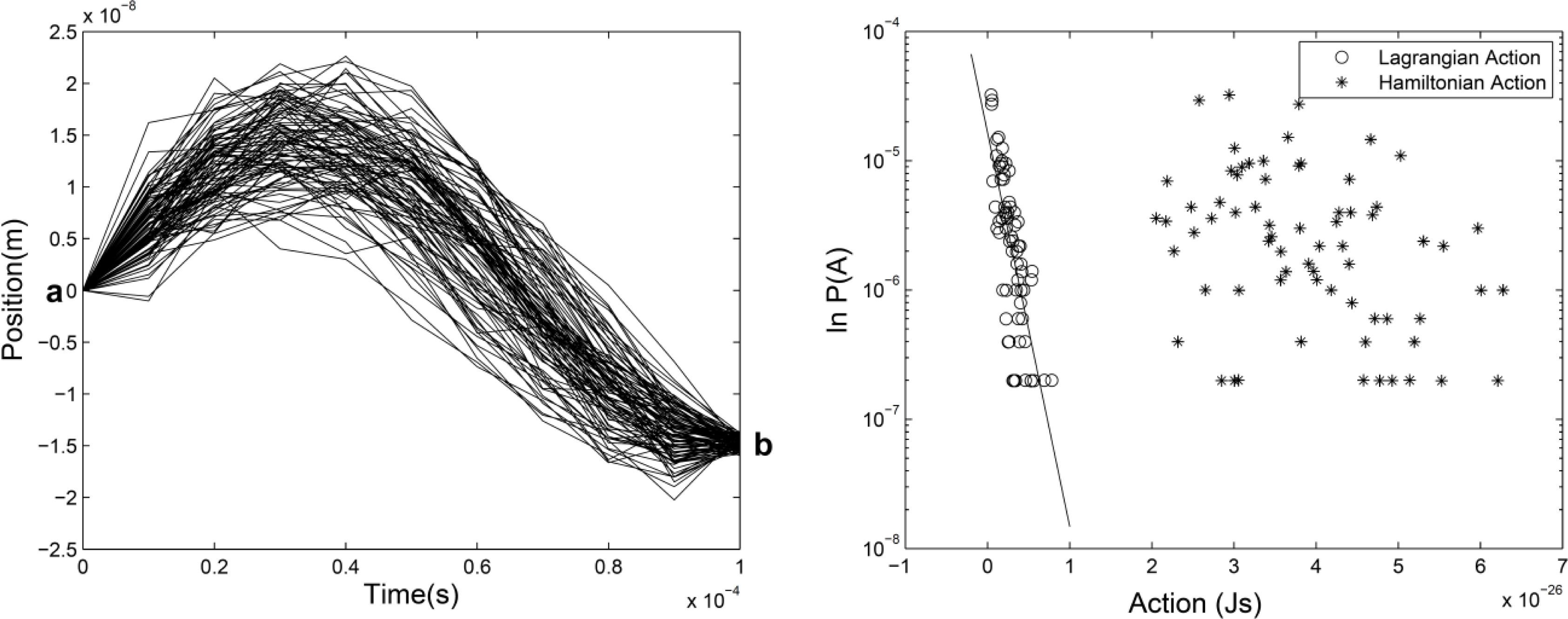
It is well known that for regular motion obeying Newtonian mechanics, the path between two given points in configuration space as well as in phase space when the time period is specified is unique [1]. However, it is not the case for random dynamics with a well-known example: Brownian motion. One of the remarkable characteristics of this motion is the non uniqueness of paths between two given points for given time period, which is illustrated in Figure 1 (left).
This phenomenon naturally raises the following questions. What is the probability for a particle, moving between two points, to take a given path or to follow a thin bundle of paths among many others? What are the variables of this probability? How to quantify the dynamical uncertainty in the path probability? Although the path probability of random motion has been noticed since longtime ago [2,3], explicit study of the expression of the path probability and its random variables is relatively new. There are different viewpoints on the question [4–7] which do not always agree with each other. In a recent work [8], the path probability of an ideal random motion was studied by numerical simulation with particles subject to conservative force and Gaussian noise. This model is ideal since the random motion statistically conserves its mechanical energy in such a way that the Hamiltonian can make sense, such as in a thermodynamically isolated system with internal fluctuation. In practice, any mechanical system with weak dissipation (or friction) can be approximately described by this model within the period in which the energy dissipated is much smaller than the energy of the motion. Figure 1 gives an example of the results. The exponential dependence of the path probability on the action is obvious from this result. The action is denoted by Ak (a,b) for a given path k between two fixed points a and b with the usual definition where K is the kinetic energy and V the potential energy along the path. In that work, we called it Lagrangian action to distinguish it from the integral of Hamiltonian (along the same path (called Hamiltonian action in that work) used to compare the action and energy correlation of the path probability. The result in the right panel of Figure 1 can be expressed by:
In this paper, we present some theoretical consequences of this numerical result. The main point is that this result implies a modification of Liouville’s theorem of conservation of phase volume due to the modification of Hamiltonian equations, which results in other important consequences relative to the entropy of thermodynamics.
2. Stochastic Least Action Principle
Let’s first see the probabilistic uncertainty, or randomness, in the choice of paths by the motion. This uncertainty is represented by the distribution Equation (1) and can be measured by the Shannon information formula . Let’s call it path entropy. It is easy to calculate:
3. Hamiltonian Mechanics Revisited
It has been shown that the exponential probability distribution of action satisfied the Fokker-Planck equation for normal diffusion in the same way as the Feymann factor of quantum propagator Pk ∝ e−iAk/ℏ satisfies the Schrödinger equation [9] Here we will show a generalized formalism of Hamiltonian mechanics whose equations will be used in the discussion of the Liouville theorem and Boltzmann H theorem.
3.1. Euler-Lagrange Equations
A meaning of the SAP Equation (3) is that for any particular path k, there is no necessarily δAk = 0. In general we have:
The Legendre transformation along a path k implies the momentum given by which can be put into Equation (5) to have:
However, from the path average of Equation (4) and the SAP , we straightforwardly write:
This is the Euler-Lagrange equation of the random dynamics. We have equivalently:
3.2. Hamiltonian Equations
From Legendre transformation, we can have and the following Hamiltonian equations:
Naturally, Equation (8) means:
4. Liouville’s Theorem
Liouville’s theorem is often involved in the discussions relative to thermodynamic entropy in statistical mechanics. We give an outline below followed by an analysis of the theorem within the present formulation of (probabilistic) Hamiltonian mechanics.
We look at the time change of phase point density ρ(x, P, t) in a, say, 2-dimensional phase space Γ when the system of interest moves on the path of least action [3] ρ(x, P, t) can also be considered as the density of systems of an ensemble of a large number of systems moving in phase space. The time evolution neither creates nor destroys state points or systems, hence the law of state conservation in the phase space is:
For the least action path satisfying Hamiltonian equations [1], the right hand side of the above equation is zero, leading to the Liouville’s theorem:
The second law of thermodynamics states that the entropy of an isolated system increases or remains constant in time. But Liouville’s theorem implies that if the motion of the system obeys the fundamental laws of mechanics, the Boltzmann entropy defined by S = lnΩ must be constant in time. On the other hand, the probability distribution of states p(x,P) in phase space is proportional to ρ(x,P), meaning that an entropy S(p), as a functional of p(x,P), must be constant in time, which is in contradiction with the second law.
What is then the Liouville’s theorem in the context of random dynamics? From Equation (13), we have along a path k. Let us write the second equation of the Equations (10) as where Rk ≥(or≤) 0 for δAk ≥(or≤) 0 is the random force causing the deviation from Newtonian laws. The average Newtonian law yields for any moment of the process. We then have:
Now let us see an application to the case of exponential path probability. The relationship implies . By using the exponential distribution of action, we have where (suppose x(t0) = 0) where xk(t) is the displacement of the motion along the path k from t0 to t. Hence where is the average of the work performed by the random forces Rk (independent from time) over the displacement xk(t). Finally, here is the cumulate average work of the random force performed from t0 and t.
We have:
If the average work does not depend on time over a process, we can write W(t,t0)=α(t−t0) and:
5. Boltzmann H Theorem
The Boltzmann H function can be defined in discrete coarse graining way in phase space by:
We have:
It is straightforward to see that the variation of H function from t0 to t is given by ΔH = H(t) − H(t0) = −γW(t,t0). Since γ is positive, it is necessary to prove that the cumulate work WR(t,t0) is positive in order to yield Boltzmann H theorem ΔH ≤ 0.
Here we only provide a proof for W(t,t0) ≥ 0 in the case of ideal gas in which each molecule can be considered as a particle in random motion. The motion of the ensemble of particles is also random, perturbed by internal fluctuation.
Let us consider the free expansion of ideal gas between two equilibrium states at time t1 and t2 with volume V1 and V2, respectively. Let p(x1, P1,t1) and p(x2, P2,t2) be the two equilibrium distributions. We use the entropy expression:
For the two equilibrium states, it is straightforward to calculate (let the Boltzmann constant kB=1):
Hence the variation of H function is , meaning that . This is a proof for the H theorem in the special case of ideal gas expansion between two equilibrium states. For the motion between any two states, the property W(t,t0) ≥0 needs a more general proof from its definition above Equation (19).
6. Concluding Remarks
We have studied the theoretical consequences of the path probability exponentially depending on action which was an observed result in the numerical experiment of random motion of Hamiltonian systems. We have indicated that this probability was an emblem of the stochastic mechanics based on a generalization of the least action principle of the classical Hamiltonian/Lagrangian mechanics. Then we have proved a modification of Liouville’s theorem within this generalized mechanics theory for the random dynamics: the distribution function of states in phase space is no more a constant in time as prescribed by Liouville’s theorem before for deterministic dynamics of Hamiltonian systems. The Boltzmann H function can have time evolution allowing entropy increase. This increase can be proved to be a consequence of the work of random forces on the systems. For the special case of free expansion of ideal gas, this random work could be identified through the increase of entropy. More general proof of the H theorem from the definition of the work of random forces can be expected.
The essential idea of this work is to derive Boltzmann’s H theorem, initially proposed to treat thermodynamic phenomena, within a mechanical theory for random motion and on the basis of a characteristic law of random dynamics: the path probability. Although this path probability has been found, by numerical simulation [8], only for a special and ideal random motion of Hamiltonian systems which statistically conserve their energy, the philosophy and the methodology should be suitable for discussing random dynamics and concomitant phenomena.
One of the aims of this work is to question the criticisms of the H theorem by Loschmidt, Poincaré and Zermelo [14–16] on the basis of the time reversible Hamiltonian mechanics and Liouville’s theorem for regular and deterministic mechanical motion. Indeed, using Liouville’s theorem to criticize H theorem, one should take it for granted that the state density is proportional to the probability distribution of states. Yet Liouville’s theorem holds only for regular dynamics in which each trajectory can be a priori traced in time with certainty, each state has its unique moment of time to be visited by the system, and the frequency of visit of any phase (state) volume can be predicted exactly. Therefore, when Liouville’s theorem holds, a priori there is no place for probability and entropy or other uncertainty in regular dynamics. On the other hand, all thermodynamic systems undergo random motion with more or less fluctuation and are intrinsically probabilistic and unpredictable. Without introducing probability and unpredictability into the basic laws of the Newtonian mechanics, any effort to relate the second law of thermodynamics to the Newtonian mechanics [17] must encounter the gap between the world of regular, deterministic, predictable and time reversible motion and the world of random, indeterministic, unpredictable and irreversible motion. As is well known Boltzmann has tried to prove the second law of thermodynamics from the H-theorem with the assumption “molecular chaos” (Stosszahlansatz) in formulating the collision term [18]. Boltzmann believes that from this assumption it is possible to break time-reversal symmetry, necessary for the entropy increase, and to solve the Loschmidt paradox [17], but Liouville’s theorem still persists and forbids the H function to change in time.
This work is an effort to generalize the regular Newtonian mechanics into a stochastic mechanics theory through path probability which is a universal character and an emblem of all random dynamics. Within the formalism with the path probability depending on action, Liouville’s theorem has to be modified to allow time evolution of the phase density as is shown in Equation (18). On the other hand, the time reversibility does not exist for Equation (5) or (10) or since the time symmetry along any path k is broken down by the random force Rk whose integration in opposite direction of time should be a priori different.
It should be stressed again that the present work is just a first generalization of Hamiltonian mechanics with an ideal model of random motion: a Hamiltonian system undergoing random motion without, statistically, loss of energy through dissipation. For the time being, this same approach, based on the least action principle, cannot be applied to dissipative systems for which this principle is no more valid. The extension of the least action principle to dissipative system is still under progress [19].
Conflicts of Interest
The authors declare no conflict of interest
References
- Arnold, V.I. Mathematical Methods of Classical Mechanics, 2nd ed; Springer-Verlag: New York, NY, USA, 1989; p. 243. [Google Scholar]
- Onsager, L; Machlup, S. Fluctuations and irreversible processes. Phys. Rev 1953, 91, 1505. [Google Scholar]
- Freidlin, M.I.; Wentzell, A.D. Random Perturbation of Dynamical Systems; Springer-Verlag: New York, NY, USA, 1984. [Google Scholar]
- Evans, R.M.L. Detailed balance has a counterpart in non-equilibrium steady states. J. Phys. Math. Gen 2005, 38, 293. [Google Scholar]
- Abaimov, S.G. General formalism of non-equilibrium statistical mechanics a path approach. 2009. arXiv:0906.0190. [Google Scholar]
- Cohen, E.G.D; Gallavotti, G. Note on two theorems in nonequilibrium statistical mechanics. 1999. arXiv:cond-mat/9903418 v1. [Google Scholar]
- Sevick, E.M.; Prabhakar, R.; Williams, S.R.; Searles, D.J. Fluctuations theorems. Annu. Rev. Phys. Chem 2008, 59, 603–633. [Google Scholar]
- Lin, T.L.; Wang, R.; Bi, W.P.; El Kaabouchi, A.; Pujos, C.; Calvayrac, F.; Wang, Q.A. Path probability distribution of stochastic motion of non dissipative systems: a classical analog of Feynman factor of path integral. Chaos Soliton. Fract 2013, 57, 129–136. [Google Scholar]
- Feynman, R.P.; Hibbs, A.R. Quantum Mechanics and Path Integrals; McGraw-Hill Publishing Company: New York, NY, USA, 1965. [Google Scholar]
- Wang, Q.A. Maximum path information and the principle of least action for chaotic system. Chaos Soliton. Fract 2004, 23, 1253–1258. [Google Scholar]
- Wang, Q.A. Non quantum uncertainty relations of stochastic dynamics. Chaos Soliton. Fract 2005, 26, 1045–1052. [Google Scholar]
- Wang, Q.A. Maximum entropy change and least action principle for nonequilibrium systems. Astrophys. Space Sci 2006, 305, 273. [Google Scholar]
- Wang, Q.A.; Tsobnang, F.; Bangoup, S.; Dzangue, F.; Jeatsa, A.; Le Méhauté, A. Reformulation of a stochastic action principle for irregular dynamics. Chaos Soliton. Fract 2009, 40, 2550–2556. [Google Scholar]
- Grandy, W.T., Jr. Entropy and the Time Evolution of Macroscopic Systems; Oxford University Press: Oxford, UK, 2008; pp. 142–152. [Google Scholar]
- Poincaré, H. Thermodynamique; Gauthier-Villars: Paris, France, 1908; pp. 449–450. [Google Scholar]
- Poincaré, H. On the Three-body Problem and the Equations of Dynamics (Sur le Probleme des trios corps ci les equations de dynamique). Acta mathematica 1890, 13, 270. [Google Scholar]Kinetic Theory of Gases; Brush, Stephen G., Hall, Nancy S., Eds.; Imperial College Press: London, UK, 2003; pp. 368–381.
- Stenger, I. Cosmopolitiques; La découverte: Paris, France, 2003; p. 169. [Google Scholar]
- Dorfman, J.R. An introduction to chaos in nonequilibrium statistical mechanics; Cambridge University Press: Cambridge, UK, 1999. [Google Scholar]
- Lin, T.L.; Wang, Q.A. The extrema of an action principle for dissipative mechanical systems. J. Appl. Mech 2013, 81, 031002. [Google Scholar]

© 2014 by the authors; licensee MDPI, Basel, Switzerland This article is an open access article distributed under the terms and conditions of the Creative Commons Attribution license (http://creativecommons.org/licenses/by/3.0/).
Share and Cite
Wang, Q.A.; El Kaabouchiu, A. From Random Motion of Hamiltonian Systems to Boltzmann’s H Theorem and Second Law of Thermodynamics: a Pathway by Path Probability. Entropy 2014, 16, 885-894. https://doi.org/10.3390/e16020885
Wang QA, El Kaabouchiu A. From Random Motion of Hamiltonian Systems to Boltzmann’s H Theorem and Second Law of Thermodynamics: a Pathway by Path Probability. Entropy. 2014; 16(2):885-894. https://doi.org/10.3390/e16020885
Chicago/Turabian StyleWang, Qiuping A., and Aziz El Kaabouchiu. 2014. "From Random Motion of Hamiltonian Systems to Boltzmann’s H Theorem and Second Law of Thermodynamics: a Pathway by Path Probability" Entropy 16, no. 2: 885-894. https://doi.org/10.3390/e16020885
APA StyleWang, Q. A., & El Kaabouchiu, A. (2014). From Random Motion of Hamiltonian Systems to Boltzmann’s H Theorem and Second Law of Thermodynamics: a Pathway by Path Probability. Entropy, 16(2), 885-894. https://doi.org/10.3390/e16020885