Image Fusion Based on the \({\Delta ^{ - 1}} - T{V_0}\) Energy Function

Abstract

This article proposes a Δ⁻¹ – TV₀ energy function to fuse a multi-spectral image with a panchromatic image. The proposed energy function consists of two components, a TV₀ component and a Δ⁻¹ component. The TV₀ term uses the sparse priority to increase the detailed spatial information; while the Δ⁻¹ term removes the block effect of the multi-spectral image. Furthermore, as the proposed energy function is non-convex, we also adopt an alternative minimization algorithm and the L₀ gradient minimization to solve it. Experimental results demonstrate the improved performance of the proposed method over existing methods.

1. Introduction

With the application of multi-source imaging in many areas, such as remote sensing [1,2], medical imaging [3] and quality and defect detection [4], image fusion has become an attractive and important research area in image processing. More specifically, in remote sensing, there is a significant interest in the fusion of high spatial and high spectral resolution images to provide a better description and visual representation of a scene. However, typically, both high spatial and spectral resolution images are not simultaneously presented in a single image, due to commercial constraints. More specifically, panchromatic images contain high spatial resolution with limited spectral resolution, while multi-spectral images contain high spectral resolution with low spatial resolution.

Consequently, many researchers have expressed interest in the fusion of multi-spectral images and panchromatic images. The most common methods are based on the intensity-hue-saturation (IHS) transform [5,6]. However, using the IHS method results in spectral degradation. To solve this problem, some algorithms based on the wavelet transform are proposed. Wavelet transform is an important tool in signal processing [7] and image processing [8,9], especially for image fusion. Núñez et al. [10] fused a high spatial resolution panchromatic image (Satellite pour l’ observation de la Terre (SPOT)) with a low spatial resolution multi-spectral image (Landsat Thematic Mapper (TM)) using the additive wavelet algorithm (AW). The Atrous wavelet approximation of the SPOT panchromatic image is substituted by the bands of TM image. Li et al. [11] proposed a choose-max wavelet fusion algorithm (CMW) based on the wavelet transform. An algorithm based on the multi-scale first fundamental form (MFF) was presented by Scheunders [12], which used a multi-valued image wavelet representation method to fuse images. However, this method is prone to large wavelet coefficients. Chen et al. [13] addressed this issue by proposing a weighted multi-scale first fundamental form method (WMFF). The image fusion methods based on wavelet transform, while reporting good results, have three limitations: empirical selection of the predefined basis; selection of the decomposition level; the wavelet method focuses on preserving spectral information. In order to solve these issues, techniques, such as the TV (total variation)–L₁ model [14–16], were proposed as a balanced spatial and spectral information model, which use the primal-dual algorithm and Bregman-splitting algorithm to maximize the matching measurement. In the TV − L₁ model, the TV regularization preserves the discontinuity of the magnitudes of gradient difference; and the L₁ data term tends to measure the low frequency information by calculating the difference between the result and the multi-spectral image. Another class of literature utilizes population-based optimization to fuse multiple images. Saeedi [17] utilized the population-based optimization to select the weights of the low-frequency wavelet coefficients to improve the infrared and visible image fusion. Saeedi [18] found the optimal pan-sharpened image by applying the multi-objective particle swarm optimization algorithm and using the two initial pan-sharpened results generated by two different fusion rules. Finally, Lacewell [19] used genetic algorithms to get a more optimized combined image for visual and thermal satellite image fusion. While the reported literature produces good results, the multi-spectral images are prone to the block effect, and the existing literature does not address this problem. In this article, we propose to address the block effect within the multi-spectral images by using the TV₀ − Δ⁻¹ energy function. The Δ⁻¹ component not only deletes the block effect, but also retains the spectral information. Additionally, the L₀ gradient term of the proposed energy function increases the spatial resolution within the final fused result.

The contributions of our paper in image fusion can be summarized as follows:

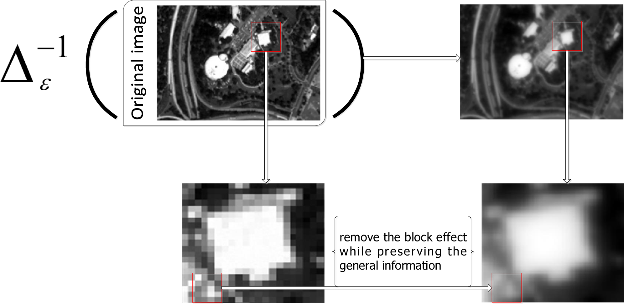
• The Δ⁻¹ term within the fusion energy function is proposed to remove the block effect in multi-spectral images without affecting the spatial information.
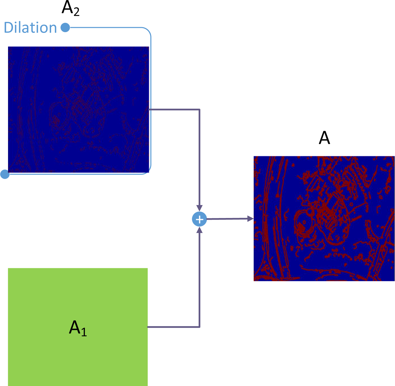
• To improve the image fusion accuracy, an alternative minimization algorithm using a non-convex L₀ regularization term is proposed.

The rest of the paper is organized as follows: Section 2 presents a detailed description of the proposed fusion algorithm. Section 3 provides experimental results and discussions on IKONOS and QUICKBIRD images. Finally, in Section 4, our conclusions are discussed.

2. Computational Method

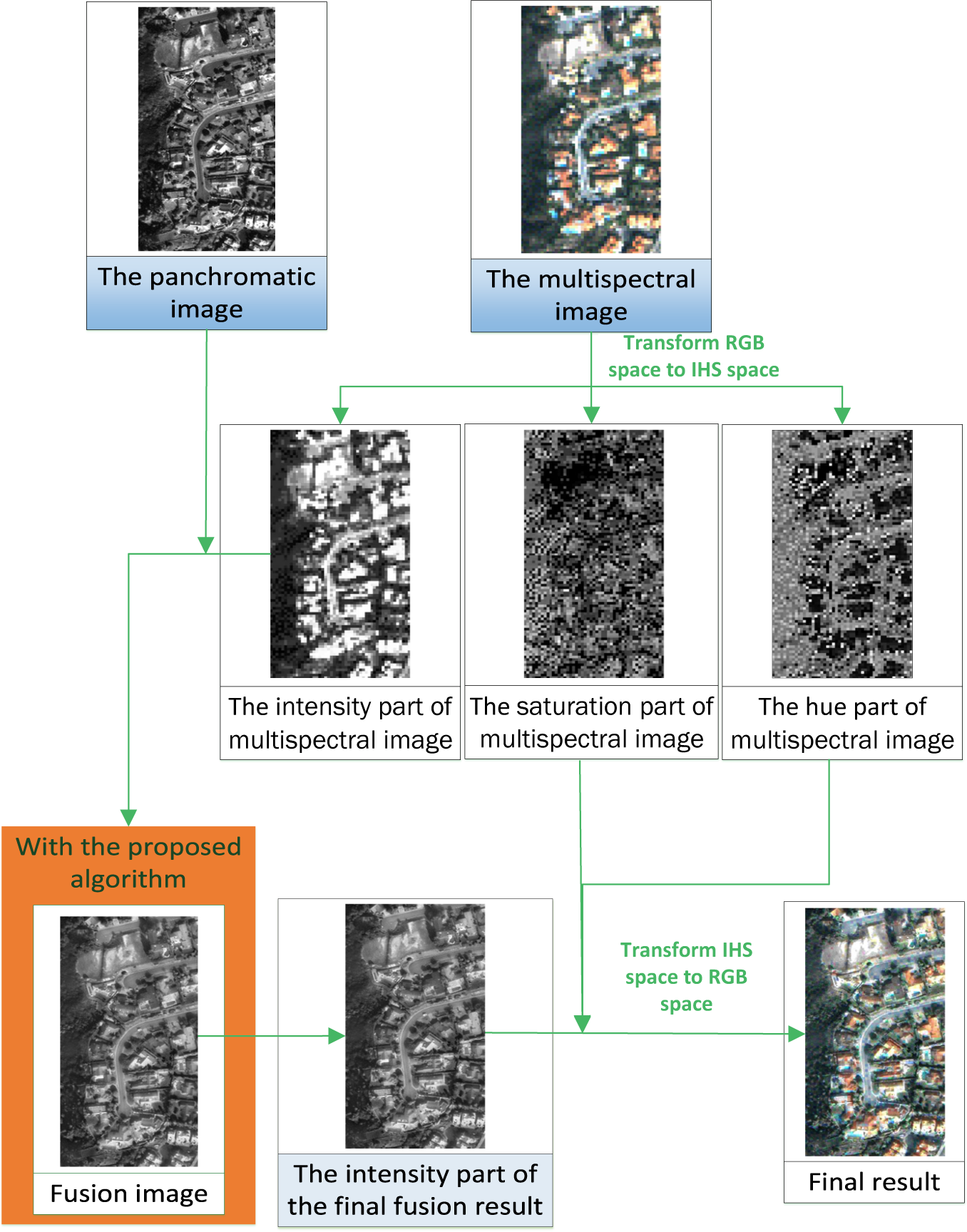
2.1. Flowchart of the Proposed Algorithm

The flowchart of the proposed algorithm is presented in Figure 1. In the proposed algorithm, the color multi-spectral image is transformed into the IHS color model [20]. The intensity component is selected as the primary fusion variable. The method uses an energy minimization process solved by an iterative process, which is based on the inverse Laplace transform and sparse norm of the gradient term.

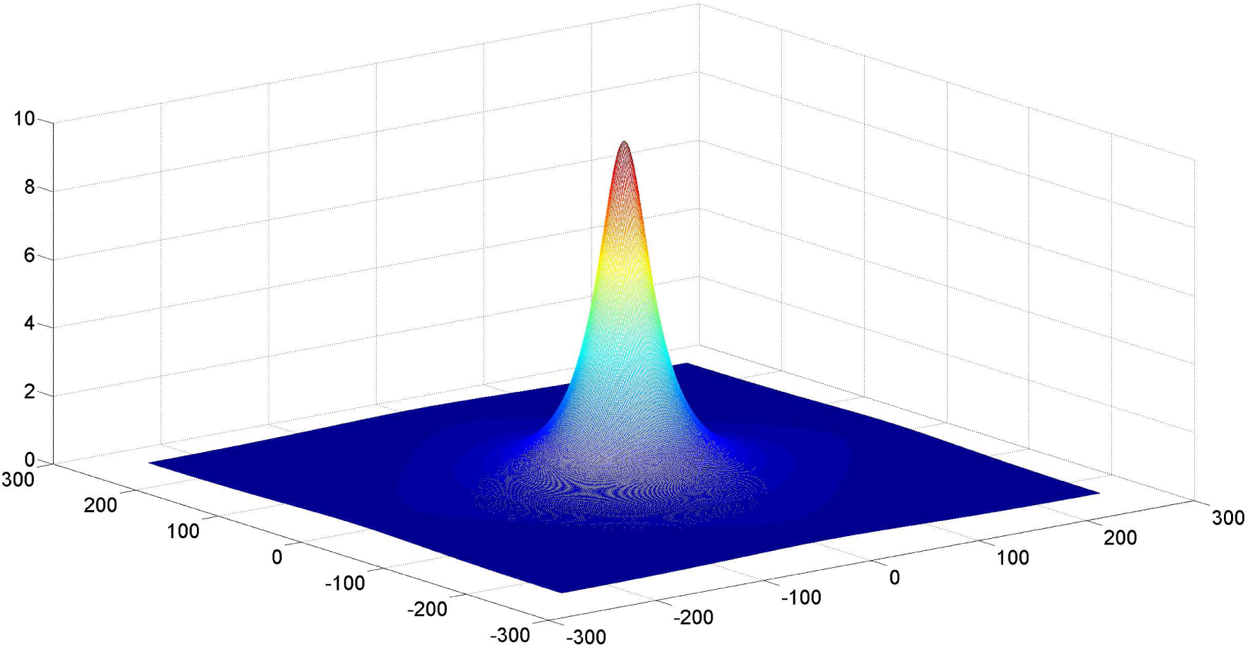
2.2. Inverse Laplace Transform Δ⁻¹

The Δ⁻¹ operator is proposed by [21,22] and also applied to image fusion quality assessment [16,23]. Additionally, [22] computes Δ⁻¹ by discrete Fourier transform. The discrete Δ operator is given by:

$$\mathrm{\Delta }f(m,n)=f(m+1,n)+f(m-1,n)+f(m,n+1)+f(m,n-1)-4f(m,n),$$

(1)

where m and n are the pixel position of image f with size [M,N]. Applying the discrete Fourier transform on (1), we obtain:

$$F(\mathrm{\Delta }f)(p,q)=2\left(\cos \left(\frac{2\pi }{M}p\right)+\cos \left(\frac{2\pi }{N}p\right)-2\right)F(f)(p,q),$$

(2)

where p and q are discrete Fourier sample points and F presents the discrete Fourier transform. In order to avoid singularity, we input a small constant ϵ and obtain the Δ⁻¹ as follows:

$${\mathrm{\Delta }}^{-1}(f)=F^{-1}\left(\frac{F(f)}{2(\cos (\frac{2\pi }{M}p)+\cos (\frac{2\pi }{N}q)-2-\epsilon )}\right).$$

(3)

As shown in Figure 2, the weighting function $\left(\frac{1}{2(\cos (\frac{2\pi }{M}p)+\cos (\frac{2\pi }{N}q)-2-\epsilon )}\right)$ of Equation (3) focuses on the low frequency component of the image f. An example of the application Δ⁻¹ on the IKONOS’s image is shown in Figure 3. It can be seen that Δ⁻¹ removes the block effect, while preserving the general information.

2.3. Functional Form

Xie et al. [14] proposed a TV − L₁ fusion method as follows:

$$\underset{R}{\min }J(R)=\underset{R}{\min }{\Vert R-T\Vert }_1+\lambda {\Vert \nabla (R-G)\Vert }_1,$$

(4)

where J is an energy function about the fusion result R, G is a panchromatic image, T is the intensity part of IHS transformation of a multi-spectral image, λ is a weighted parameter and ${\Vert \nabla \cdot \Vert }_1$ stands for a discrete total variation norm. If we use the anisotropic total variation form, we can transform Equation (4) as follows:

$$\underset{R}{\min }J(R)=\underset{R}{\min }{\Vert R-T\Vert }_1+\lambda {\Vert R_x-G_x\Vert }_1+\lambda {\Vert R_y-G_y\Vert }_1,$$

(5)

where R_x is the partial derivative of R with respect to x, R_y is the partial derivative of R with respect to y, G_x is the partial derivative of G with respect to x and G_y is the partial derivative of G with respect to y.

In recent years, many studies have empirically demonstrated through experiments that non-convex potential functions are suitable for optimization-based computer vision problems. Krishnan [24] used a normalized sparsity measure similar to L₀ for the image blind deconvolution model. A L_p norm [25] is proposed to solve the optical flow and image denoising model. Fu and Zhang [26] proposed an adaptive non-convex model to solve the image restoration model. Consequently, in our article, we investigate the use of a sparse L₀ norm to increase the image details of the fused result. A non-convex L₀ norm is substituted for the L₁ norm of anisotropic total variation of the TV − L₁ model as follows:

$$\underset{R}{\min }J(R)=\underset{R}{\min }{\Vert R-T\Vert }_1+\lambda {\Vert R_x-G_x\Vert }_0+\lambda {\Vert R_y-G_y\Vert }_0,$$

(6)

where ${\Vert R_y-G_y\Vert }_0=\oplus \langle p,|R_{y,p}-G_{y,p}|\ne 0\rangle$, p is the pixels and ⊕ is the counting operator. We use the L₀ norm of the gradient to transform the spatial information, which can retain the spectral information, whose tendency is inconsistent with the spatial information.

While the TV − L₁ model demonstrates good results for multi-spectral fusion, the final fused images contain the block effect, as discussed earlier. To address this issue, we apply Δ⁻¹ on the data fitting term and substitute ||R − T||₁ with ||Δ⁻¹R − Δ⁻¹T||₁ as:

$$\underset{R}{\min }J(R)=\underset{R}{\min }{\Vert {\mathrm{\Delta }}^{-1}R-{\mathrm{\Delta }}^{-1}T\Vert }_2^2+\lambda {\Vert R_x-G_x\Vert }_0+\lambda {\Vert R_y-G_y\Vert }_0,$$

(7)

where R is the fused result, which retains the spatial information and the spectral information. Moreover, we employ the Δ⁻¹ operator, within ||TV − L₁|| as ||Δ⁻¹R − Δ⁻¹T||₁, resulting in the function focusing on the low frequency information of R − T and neglecting the high frequency information.

Finally, as Model (7) is a non-convex model, we solve the problem using an alternative minimization algorithm, as detailed in the next subsection.

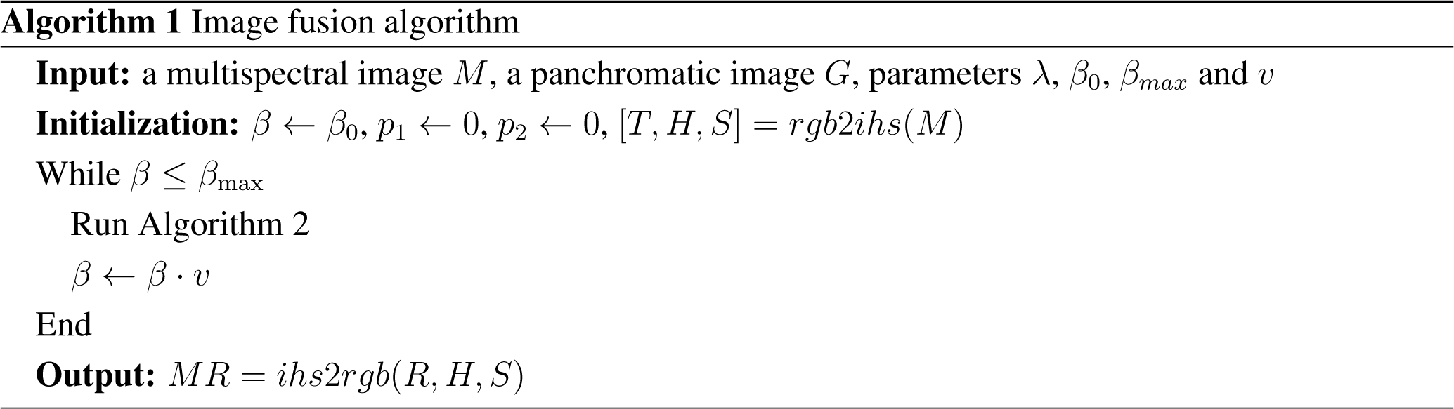
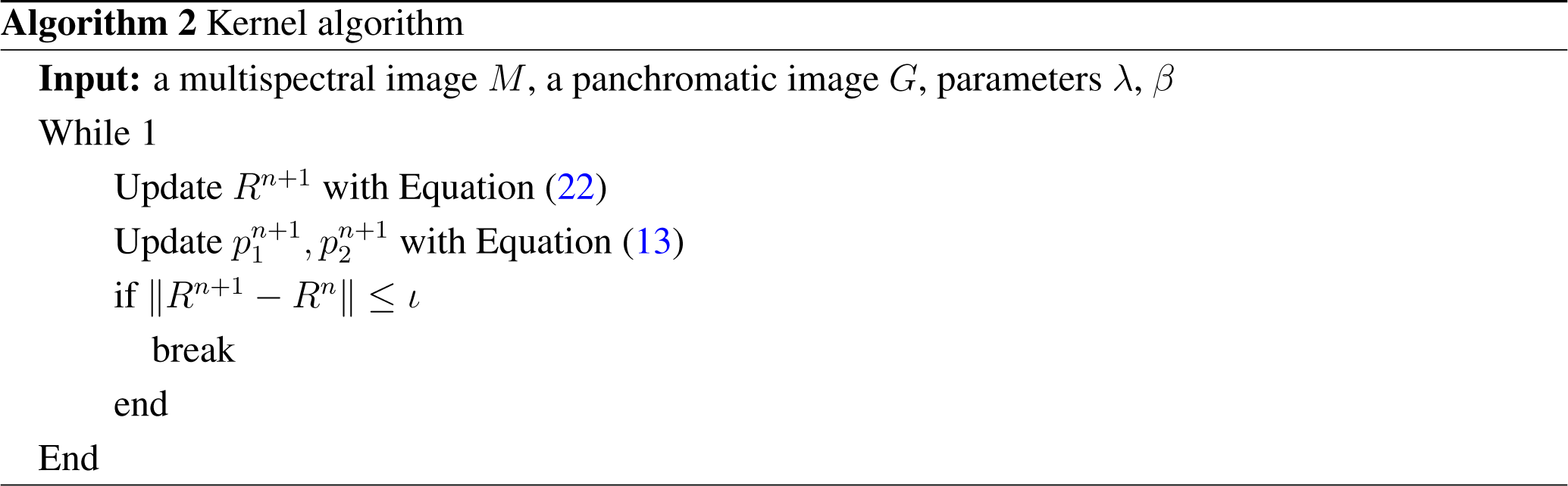
2.4. Alternative Minimization Algorithm

We use the splitting scheme similar to [20,27] to solve Equation (7). It is well-known that the L₀ problem is strongly NP-hard to solve, but we solve it based on the conclusion reported in [26]. Firstly, we introduce two auxiliary variables p₁ and p₂ to transform Model (7) as follows:

$$\begin{array}{c}\underset{R,p_1,p_2}{\min }J(R,p_1,p_2)=\underset{R,p_1,p_2}{\min }{\Vert {\mathrm{\Delta }}^{-1}R-{\mathrm{\Delta }}^{-1}T\Vert }_2^2+\beta {\Vert R_x-G_x-p_1\Vert }_2^2+\\ \beta {\Vert R_y-G_y-p_2\Vert }_2^2+\lambda {\Vert p_1\Vert }_0+\lambda {\Vert p_2\Vert }_0.\end{array}$$

(8)

The alternative minimization algorithm [28] is employed to solve Model (8). The most important part of the alternative minimization is to solve:

$$\begin{array}{l}{\min }_{p_1}{J}_1(p_1)=\beta {\Vert R_x-G_x-p_1\Vert }_2+\lambda {\Vert p_1\Vert }_0\\ {\min }_{p_2}{J}_1(p_2)=\beta {\Vert R_y-G_y-p_2\Vert }_2+\lambda {\Vert p_2\Vert }_0.\end{array}$$

(9)

It is well known that Model (9) is strongly NP-hard. We use the technique of [27] to decompose it into the following model:

$$\begin{array}{l}{\displaystyle \sum _i{\min }_{p_{1,i}}\{\beta {(R_{x,i}-G_{x,i}-p_{1,i})}^2+\lambda H(|p_{1,i}|)\}}\\ {\displaystyle \sum _i{\min }_{p_{2,i}}\{\beta {(R_{y,i}-G_{y,i}-p_{2,i})}^2+\lambda H(|p_{2,i}|)\}},\end{array}$$

(10)

where i is the pixel position of the image and H is defined as:

$$H(|x|)=\{\begin{array}{c}1,\text{if}|x|\ne 0;\\ 0,\text{otherwise}.\end{array}$$

(11)

Next, Model (9) is rewritten by Model (10). Additionally, solve Model (10) by computing each term as follows:

$$\begin{array}{l}{\min }_{p_{1,i}}\left\{{(R_{x,i}-G_{x,i}-p_{1,i})}^2+\frac{\lambda }{\beta }H(|p_{1,i}|)\right\}\\ {\min }_{p_{2,i}}\left\{{(R_{y,i}-G_{y,i}-p_{2,i})}^2+\frac{\lambda }{\beta }H(|p_{2,i}|)\right\}.\end{array}$$

(12)

To solve Model (12), we need Proposition 1.

Proposition 1. Model (12) obtains the minimum under the conditions:

$$\begin{array}{l}\begin{array}{cc}{p}_{1,i}=\{\begin{array}{c}0,\\ R_{y,i}-G_{y,i}\end{array}& \begin{array}{c}{(R_{y,i}-G_{y,i})}^2\le \frac{\lambda }{\beta };\\ otherwise\end{array}\end{array}\\ \begin{array}{cc}{p}_{2,i}=\{\begin{array}{c}0,\\ R_{y,i}-G_{y,i}\end{array}& \begin{array}{c}{(R_{x,i}-G_{x,i})}^2\le \frac{\lambda }{\beta };\\ otherwise\end{array}\end{array}\end{array}$$

(13)

The proof is similar to [27]. In order for this paper to be self-contained, we present the proof of Proposition 1 as follows.

Proof. If ${(R_{x.i}-G_{x,i})}^2\le \frac{\lambda }{\beta }$ and p_1,i ≠ 0, we have:

$$\begin{array}{c}{(R_{x,i}-G_{x,i}-p_{1,i})}^2+\frac{\lambda }{\beta }H(|p_{1,i}|)={(R_{x,i}-G_{x,i}-p_{1,i})}^2+\frac{\lambda }{\beta }\\ \ge \frac{\lambda }{\beta }\\ \ge {(R_{x,i}-G_{x,i})}^2.\end{array}$$

(14)

If ${(R_{x,i}-G_{x,i})}^2\le \frac{\lambda }{\beta }$ and p_1,i = 0, we have:

$${(R_{x,i}-G_{x,i}-p_{1,i})}^2+\frac{\lambda }{\beta }H(|p_{1,i}|)={(R_{x,i}-G_{x,i})}^2.$$

(15)

Combining (14) and (15), we conclude that if ${(R_{x,i}-G_{x,i})}^2\le \frac{\lambda }{\beta }$ and p_1,i = 0, Model (12) obtains the minimum (R_x,i − G_x,i)².

If ${(R_{x,i}-G_{x,i})}^2\le \frac{\lambda }{\beta }$ and p_1,i ≤ 0, we have:

$$\begin{array}{c}{(R_{x,i}-G_{x,i}-p_{1,i})}^2+\frac{\lambda }{\beta }H(|p_{1,i}|)={(R_{x,i}-G_{x,i}-p_{1,i})}^2+\frac{\lambda }{\beta }\\ \ge \frac{\lambda }{\beta }.(\text{If}{p}_{1,i}=R_{x,i}-G_{x,i},theequalityholds.)\end{array}$$

(16)

If ${(R_{x,i}-G_{x,i})}^2>\frac{\lambda }{\beta }$ and p_1,i = 0, we obtain:

$${(R_{x,i}-G_{x,i}-p_{1,i})}^2+\frac{\lambda }{\beta }H(|p_{1,i}|)={(R_{x,i}-G_{x,i})}^2.$$

(17)

Combining (16) and (17), we conclude that if ${(R_{x,i}-G_{x,i})}^2>\frac{\lambda }{\beta }$ and p_1,i = R_x,i − G_x,i, Model (12) obtains the minimum $\frac{\lambda }{\beta }$. Thus, we complete the proof of Proposition 1.

Because every point is considered to be a single point individual, we simplify Equation (13) as follows:

$$\begin{array}{l}\begin{array}{cc}{p}_1=\{\begin{array}{c}0,\\ R_x-G_x,\end{array}& \begin{array}{c}{(R_{y,i}-G_{y,i})}^2\le \frac{\lambda }{\beta };\\ otherwise.\end{array}\end{array}\\ \begin{array}{cc}{p}_2=\{\begin{array}{c}0,\\ R_y-G_y,\end{array}& \begin{array}{c}{(R_y-G_y)}^2\le \frac{\lambda }{\beta };\\ otherwise.\end{array}\end{array}\end{array}$$

(18)

Although Proposition 1 can solve the L₀ approximately, another sub-problem of the alternate minimization is to solve as follows:

$$\underset{R}{\min }{J}_2(R)=\underset{R}{\min }{\Vert {\mathrm{\Delta }}^{-1}R-{\mathrm{\Delta }}^{-1}T\Vert }_2^2+\beta {\Vert R_x-G_x-p_1\Vert }_2^2+\beta {\Vert R_y-G_y-p_2\Vert }_2^2.$$

(19)

Based on the definition of Δ⁻¹ and the discrete Fourier transform, we transform (19) as follows:

$$\begin{array}{c}\underset{F(R)}{\min }{J}_2(F(R))=\underset{R}{\min }{\Vert F({\mathrm{\Delta }}^{-1}R)-F({\mathrm{\Delta }}^{-1}T)\Vert }_2^2+\beta {\Vert F{({\partial }_x)}^{\circ }F(R)-F{({\partial }_x)}^{\circ }F(G)-F(p_1)\Vert }_2^2\\ +\beta {\Vert F{({\partial }_y)}^{\circ }F(R)-F{({\partial }_y)}^{\circ }F(G)-F(p_2)\Vert }_2^2,\end{array}$$

(20)

where ○ represents the element-wise multiplication. Based on (3), Equation (20) can be transformed as follows:

$$\begin{array}{l}\underset{F(R)}{\min }{J}_2(F(R))={\Vert \frac{F(R)-F(T)}{2(\cos (\frac{2\pi }{M}p)+\cos (\frac{2\pi }{N}q)-2-\epsilon )}\Vert }_2^2+\beta {\Vert F{({\partial }_x)}^{\circ }F(R)-F{({\partial }_x)}^{\circ }F(G)-F(p_1)\Vert }_2^2\\ +\beta {\Vert F{({\partial }_y)}^{\circ }F(R)-F{({\partial }_y)}^{\circ }F(G)-F(p_2)\Vert }_2^2.\end{array}$$

(21)

Then, we obtain the solution:

$$\begin{array}{l}{W}_0=\frac{1}{2(\cos (\frac{2\pi }{M}p)+\cos (\frac{2\pi }{N}q)-2-\epsilon )}\\ W_1=W_0^{†}\circ F(T)+\beta F{({\partial }_x)}^{†}\circ F{({\partial }_x)}^{†}\circ F({\partial }_x)\circ F(G)\circ F(p_1)+\beta F{({\partial }_y)}^{†}\circ F({\partial }_y)\circ F(G)\circ F(p_2)\\ W_2=W_0^{†}\circ W_0+\beta F{({\partial }_x)}^{†}\circ F({\partial }_x)+\beta F{({\partial }_y)}^{†}\circ F({\partial }_y)\\ R=F^{-1}(W_1./W_2),\end{array}$$

(22)

where ^† represents the conjugate transpose operator, ./ is the element-wise division, F⁻¹ is the inverse Fourier transform and (∂_x, ∂_y) are differentiated operators.

After we solve the above important sub-optimization, we present our framework by Algorithms 1 and 2 as follows:

Algorithm 1 Image fusion algorithm

Algorithm 1 Image fusion algorithm

Algorithm 2 Kernel algorithm

Algorithm 2 Kernel algorithm

Remark 1.

• rgb2ihs indicates the transformation from RGB (red, green, blue) space to IHS (intensity, hue, saturation) space.
• ihs2rgb indicates the transformation from IHS space to RGB space.
• ι is a small positive constant.

To give convergence results for the generated sequence ${\{J(R^i,p_1^i,p_2^i)\}}_{i\in \text{IN}}$ generated by Algorithm 2, we give Proposition 2 as follows.

Proposition 2. If ϵ > 0, the sequence$J(R^n,p_1^n,p_2^n)$ generated by Algorithm 2 converges monotonically.

Proof. Based on the Plancherel theorem, the energy of (20) is equal to the energy of (19). As Equation (22) presents, the solver of the energy Equation (19) is:

$$R^n=F^{-1}(W_1^n./W_2^n),$$

(23)

where $W_1^n=W_0^{†}\circ F(T)+\beta F{({\partial }_x)}^{†}\circ F({\partial }_x)\circ F{(G)}^{\circ }F(p_1^n)+\beta F{({\partial }_y)}^{†}\circ F({\partial }_y)\circ F(G)\circ F(p_2^n)$ and $W_2^n=W_0^{†}\circ W_0+\beta F{({\partial }_x)}^{†}\circ F({\partial }_x)+\beta F{({\partial }_y)}^{†}\circ F({\partial }_y)$. If $\forall i,j,W_2^n(i,j)\ne 0$, the solver Rⁿ⁺¹ can be obtained by the Equation (23).

If ϵ > 0, the equation $2(\cos (\frac{2\pi }{M}p)+\cos (\frac{2\pi }{N}q)-2-\epsilon )<0$ is generated. Therefore,

$$\begin{array}{l}{W}_2^n=\underset{>0}{\underbrace{W_0^{†}\circ W_0}}+\underset{\ge 0}{\underbrace{\beta F{({\partial }_x)}^{†}\circ F({\partial }_x)}}+\underset{\ge 0}{\underbrace{\beta F{({\partial }_y)}^{†}\circ F({\partial }_y)}}\\ >0.\end{array}$$

(24)

Accordingly, the optimization problem (19) can be solved. Then, we obtain that $J(R^{n+1},p_1^n,p_2^n)\le J(R^n,p_1^n,p_2^n)$. Based on Proposition 1, we obtain that $J(R^{n+1},p_1^{n+1},p_2^{n+1})\le J(R^{n+1},p_1^n,p_2^n)$. From the above discussion, we obtain that:

$$J(R^{n+1},p_1^{n+1},p_2^{n+1})\le J(R^n,p_1^n,p_2^n).$$

(25)

It is trivial to obtain that J(·,·,·) is bounded from below. With the monotone convergence theorem, the sequence ${\{J(R^i,p_1^i,p_2^i)\}}_{i\in \text{IN}}$ converges to a limit vector a.

2.5. The Selection of the Key Parameter λ

Parameter λ is very important for our fusion energy function. It determines the level of detail of information from the panchromatic image and the level of spectral information from the multi-spectral image present in the final fused image. In this paper, we do not assign a fixed value to λ, but an image A. Image A is constructed of two parts: one is a constant value matrix A1 corresponding to the previous constant parameter, and the other is the logical matrix A₂ derived from the dilation operator of the mathematical morphology on the edge image of the panchromatic image. That means if A₂(i) is larger, the object function focuses on the panchromatic image; otherwise, the multi-spectral information is considered. An example of image A is shown in Figure 4. Because Equation (13) is the point-wise operator, we can substitute the value λ with matrix A. Thus, we extend Equation (13) as follows:

$$\begin{array}{l}\begin{array}{cc}{p}_{1,i}=\{\begin{array}{c}0,\\ R_{x,i}-G_{x,i}\end{array}& \begin{array}{c}{(R_{x,i}-G_{x,i})}^2\le \frac{A(i)}{\beta };\\ otherwise.\end{array}\end{array}\\ \begin{array}{cc}{p}_{2,i}=\{\begin{array}{c}0,\\ R_{y,i}-G_{y,i}\end{array}& \begin{array}{c}{(R_{y,i}-G_{y,i})}^2\le \frac{A(i)}{\beta };\\ otherwise.\end{array}\end{array}\end{array}$$

(26)

where i is the pixel position of the image.

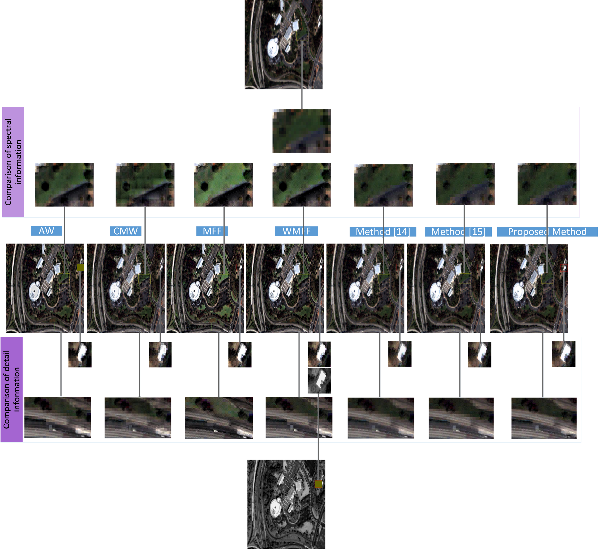
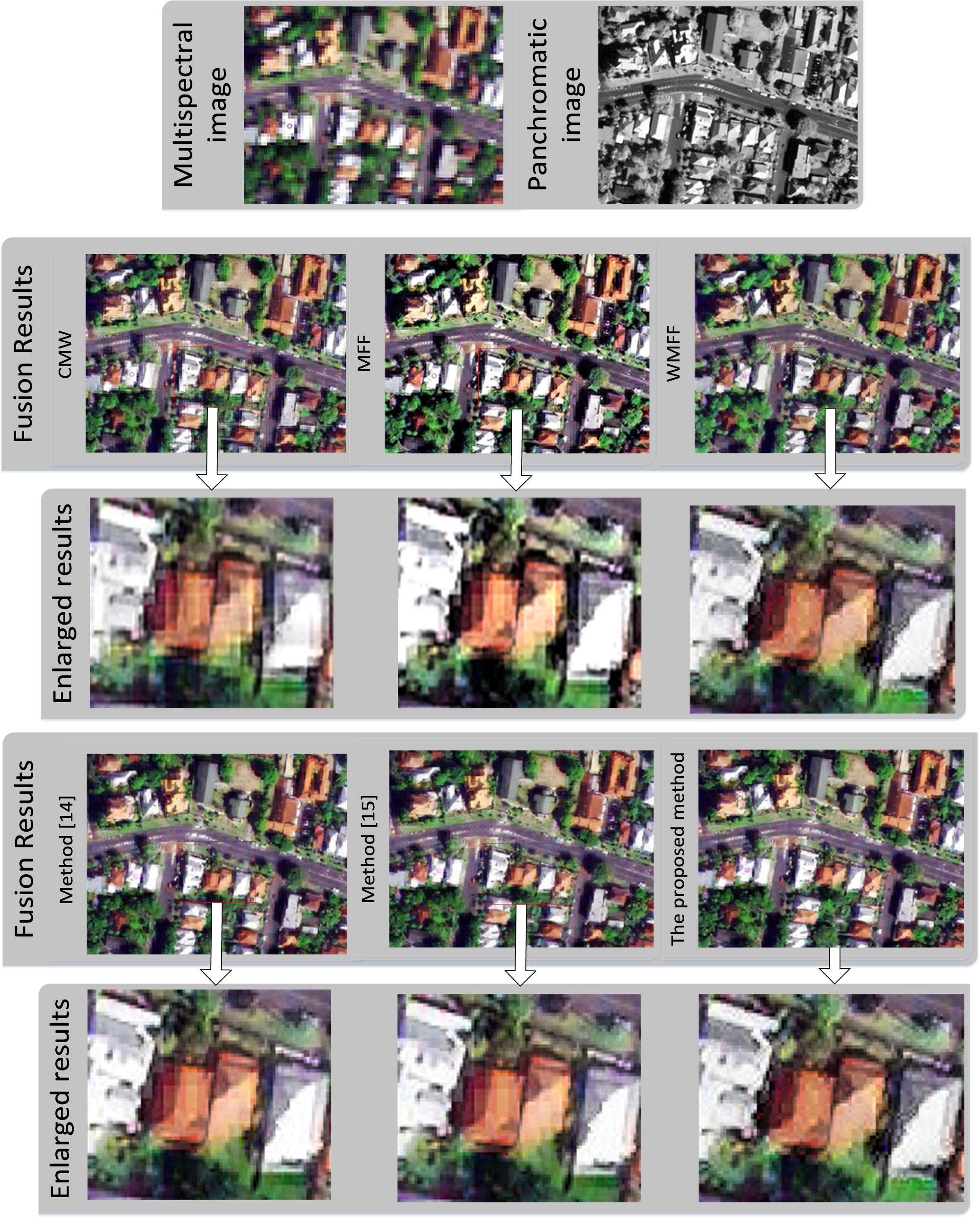
3. Experimental Results

Some experiments on IKONOS and QUICKBIRD images are used to validate the proposed algorithm. We use two metrics to quantify the performance. The correlation measure (CM) [10] is defined as follows:

$$CM(A,B)=\frac{(A-\overline{A})(B-\overline{B})}{{\Vert (A-\overline{A})\Vert }_2{\Vert (B-\overline{B})\Vert }_2},$$

(27)

where A and B are the images in the lexicographic order. CM computes correlation coefficients of the red, the green and the blue channels between the multispectral image and the fused result; this computation can be used to assess the preservation of the spectral information of the result.

A feature-based metric Q^AB/F [29] is adopted. The Q^AB/F metric is defined as follows:

$$g_A(m,n)=\sqrt{s_A^x{(m,n)}^2+s_A^y{(m,n)}^2},a_A(m,n)={\tan }^{-1}(\frac{s_A^y(m,n)}{s_A^x(m,n)}),$$

(28)

where $s_A^x(m,n)$ and $s_A^y(m,n)$ are the outputs of the horizontal and vertical Sobel templates centered on pixel (m, n) and convolved with the corresponding pixels of image A. Similarly, g_B(m, n) and g_F(m, n) can also be obtained by the above definition. The relative strength and orientation values of G^AF and A^AF of image A with respect to F are defined as:

$$G^{AF}(m,n)=\{\begin{array}{cc}\frac{g_F(m,n)}{g_A(m,n)},& \text{if}{g}_A(m,n)>g_F(m,n);\\ \frac{g_F(m,n)}{g_A(m,n)},& \text{otherwise}.\end{array}$$

(29)

$$A^{AF}(m,n)=\frac{|a_A(m,n)-a_A(m,n)|-\pi /2\left|\right|}{\pi /2}.$$

(30)

Then, the edge strength and orientation preservation values are derived as:

$$Q_g^{AF}=\frac{{\mathrm{\Gamma }}_g}{1+{\mathrm{e}}^{K_g(G^{AF}(m,n)-{\sigma }_g)}},$$

(31)

$$Q_a^{AF}=\frac{{\mathrm{\Gamma }}_a}{1+{\mathrm{e}}^{K_a(A^{AF}(m,n)-{\sigma }_a)}},$$

(32)

where Γ_g, K_g,σ_g,Γ_α, K_α and σ_α are constants and determine the exact shape of the sigmoid functions used to form the edge strength and orientation preservation values. Edge information preservation values are then defined as:

$$Q^{AF}=Q_g^{AF}{Q}_a^{AF}.$$

(33)

Therefore, Q^AB/F is obtained as:

$$Q^{AB/F}=\frac{{\displaystyle \sum _{m=1}^M{\displaystyle \sum _{n=1}^N{Q}^{AF}(m,n)w^A(m,n)+Q^{BF}(m,n)w^B(m,n)}}}{{\displaystyle \sum _{i=1}^M{\displaystyle \sum _{j=1}^N(w^A(i,j)+w^B(i,j))}}},$$

(34)

where w^A(m,n) = (g_A(m,n))^L,w^B(m,n) = (g_B(m, n))^L and L is a constant. Q^AB/F considers the amount of edge information transferred from the input images to the fused image. The larger Q^AB/F value indicates that the fused result contains more information from the input images.

Spatial frequency (SF) measurement [30,31] is about the overall activity level in an image. The spatial frequency is defined as follows:

$$RF=\sqrt{\frac{1}{M\times N}{\displaystyle \sum _{i=1}^M{\displaystyle \sum _{j=2}^N{(I(i,j)-I(i,j-1))}^2}}}$$

(35)

$$CF=\sqrt{\frac{1}{M\times N}{\displaystyle \sum _{i=2}^M{\displaystyle \sum _{j=1}^N{(I(i,j)-I(i-1,j))}^2}}}$$

(36)

$$SF=\sqrt{{(RF)}^2+{(CF)}^2},$$

(37)

where SF is defined on an M × N image I, RF is row frequency, CF is column frequency and I(i,j) denotes the samples of image. The large value of SF means that the image contains components in a high frequency area. The spatial frequent measurement can be used to reflect the clarity of the result.

The proposed method is compared to some wavelet-based methods, such as the additive wavelet fusion method (AW) [10], the choose-max wavelet fusion method (CMW) [11], the multi-scale fundamental forms fusion method (MFF) [12] and the weighted multi-scale fundamental forms fusion method (WMFF) [13]. In order to illustrate the superiority of the proposed L₀ gradient minimization, we perform a comparative experimentation with L₁ gradient minimization-based methods [14,15], and the results are shown in

Table 1. Quantitative comparison results of Figure 5. AW, additive wavelet fusion method; CMW, choose-max wavelet fusion method; MFF, multi-scale fundamental forms fusion method; WMFF, weighted multi-scale fundamental forms fusion method.

Fusion Method	CM(Red channel)	CM(Green channel)	CM(Blue channel)	QAB/F	SF
AW	0.9341	0.9345	0.9402	0.4109	0.0642
CMW	0.9426	0.9443	0.9501	0.3491	0.0640
MFF	0.8281	0.8255	0.8497	0.3700	0.0810
WMFF	0.9268	0.9265	0.9353	0.4304	0.0738
Method [14]	0.9503	0.9528	0.9558	0.4311	0.0768
Method [15]	0.9502	0.9527	0.9555	0.4157	0.0776
Proposed method	0.9505	0.9534	0.9570	0.4485	0.0842

and

Table 2. Quantitative comparison results of Figure 6.

Fusion Method	CM(Red channel)	CM(Green channel)	CM(Blue channel)	QAB/F	SF
CMW	0.8835	0.8704	0.8616	0.3576	0.1129
MFF	0.8321	0.8130	0.7980	0.3542	0.0959
WMFF	0.8920	0.8745	0.8704	0.4075	0.0941
Method [14]	0.8921	0.8850	0.8743	0.4105	0.1360
Method [15]	0.8921	0.8847	0.8746	0.4073	0.1372
Proposed method	0.8927	0.8849	0.8751	0.4260	0.1478

.

From the enlarged portion of the fused result, Figure 5 shows that our proposed algorithm has removed the block effect. We selected the parameter to make CM (r) metric, as close as possible, which means the retained spectral information is as close as possible. We applied the above metric to quantify the results in Table 1. In Table 1, CM (r), CM (g) and CM (b) correspond to the correlation measures of the red channel, the green channel and the blue channel. This shows that our fused result preserves more spectral information than the other methods. The fourth column of Table 1 illustrates that the image obtained by the proposed method gets more feature information from the original image than other methods. The sixth column of Table 1 obtained by the proposed method indicates that our method obtains clearer results than the other methods.

Figure 6 shows the fused QUICKBIRD’s images that are obtained by CMW, MMF, WMMF, the methods of [14,15] and the proposed method. The above metric is applied to quantify the results in Table 2. In Table 2, CM (r), CM (g) and CM (b) correspond to the correlation measure of the red channel, the green channel and the blue channel; this shows that our fused result preserves more spectral information than other methods. The fourth column of Table 2 illustrates that the image obtained by the proposed method gets more feature information from the original images than other methods. The sixth column of Table 1 obtained by the proposed method indicates that our method obtains clearer results than the other methods.

4. Conclusion

The proposed algorithm removes the block effect efficiently by using the Δ⁻¹ operator. In addition, we use a non-convex functional form to improve our fusion result. Simultaneously, our proposed method presents a new energy minimization algorithm to retain the spectral and high frequency information from the original images. We conduct some experiments on the IKONOS and QUICKBIRD images, and the proposed algorithm obtains a better fusion result than other fusion algorithms, in terms of not only visual quality, but also some fusion indicators.

References

1. Nichol, J.; Wong, M.S. Satellite remote sensing for detailed landslides inventories using change detection and image fusion. Int. J. Remote Sens 2005, 26, 1913–1926. [Google Scholar]
2. Schowengerdt, R.A. The nature of remote sensing. In Remote Sensing: Models and Methods for Image Processing; Academic Press: New York, NY, USA, 2006; pp. 1–44. [Google Scholar]
3. Bulanon, D.M.; Burks, T.F.; Alchanatis, V. Image fusion of visible and thermal images for fruit detection. Biosyst. Eng 2009, 103, 12–22. [Google Scholar]
4. Fischer, M.A.; Nanz, D.; Hany, T.; Reiner, C.S.; Stolzmann, P.; Donati, O.F.; Breitenstein, S.; Schneider, P.; Weishaupt, D.; Schulthess, G.K.; et al. Diagnostic accuracy of whole-body MRI/DWI image fusion for detection of malignant tumours: A comparison with PET/CT. Mol. Imaging 2011, 21, 246–255. [Google Scholar]
5. Shettigara, V.K. A generalized component substitition technique for spatial enhacement of multispectral images using a higher resolution data set. Photogramm. Eng. Remote Sens 1992, 58, 561–566. [Google Scholar]
6. Tu, T.M.; Su, S.C.; Shyu, H.C.; Huang, P.S. A new look at IHS-like image fusion methods. Inf. Fusion 2001, 2, 177–186. [Google Scholar]
7. Bayram, I.; Selesnick, I.W. A dual-tree rational-dilation complex wavelet transform. IEEE Trans. Signal Process 2011, 59, 6251–6256. [Google Scholar]
8. Demirel, H.; Anbarjafari, G. Image resolution enhancement by using discrete and stationary wavelet Decomposition. IEEE Trans. Signal Process 2011, 20, 1458–1460. [Google Scholar]
9. You, X.G.; Du, L.; Cheung, Y.M.; Chen, Q.H. A blind watermarking Scheme using new nontensor product wavelet filter banks. IEEE Trans. Signal Process 2010, 19, 3271–3284. [Google Scholar]
10. Núñez, J.; Otazu, X.; Fors, O.; Prades, A.; Pala, V.; Arbiol, R. Multiresolution based image fusion with additive wavelet decomposition. IEEE Trans. Geosci. Remote Sens 1999, 32, 1204–1211. [Google Scholar]
11. Li, H.; Manjunath, B.S.; Mitra, S.K. Multisensor image fusion using the wavelet transform. Graph. Model. Image Process 1995, 57, 235–245. [Google Scholar]
12. Scheunders, P. A multivalued image wavelet representation based on multiscale fundamental forms. IEEE Trans. Image Process 2002, 10, 568–575. [Google Scholar]
13. Chen, T.; Guo, R.S.; Peng, S.L. Image fusion using weighted multiscale fundamental form. Proceedings of IEEE International Conference on Image Processing, 24–27 October 2004; pp. 3319–3322.
14. Xie, Q.W.; He, J.C.; Long, Q.; Mita, S.; Chen, X.; Jiang, A. Image fusion based on TV − L1 function. Proceedings of the 2013 International Conference on Wavelet Analysis and Pattern Recognition, Tianjin, China, 14–17 July 2013; pp. 173–177.
15. Xie, Q.W.; Long, Q.; Mita, S.; Chen, X.; Jiang, A. Image fusion based on TV − L1 – convex constrained algorithm. Proceedings of the 2013 International Conference on Wireless Communications & Signal Processing, Hangzhou, China, 24–26 October 2013; pp. 1–5.
16. Xie, Q.W.; Long, Q.; Mita, S.; Guo, C.Z.; Jiang, A. Image fusion based on multi-objective optimization. Int. J. Wavelets Multiresolut. Inf. Process 2014, 12, 1450017. [Google Scholar]
17. Saeedi, J.; Faez, K. Infrared and visible image fusion using fuzzy logic and population-based optimization. Appl. Soft Comput 2012, 12, 1041–1054. [Google Scholar]
18. Saeedi, J.; Faez, K. A new pan-sharpening method using multi-objective particle swarm optimization and the shiftable contourlet transform. ISPRS J. Photogramm. Remote Sens 2011, 66, 365–381. [Google Scholar]
19. Lacewell, C.W.; Gebril, M.; Buaba, R.; Homaifar, A. Optimization of image fusion using genetic algorithms and discrete wavelet transform. Proceedings of IEEE conference on Aerospace and Electronics, Fairborn, OH, USA, 14–16 July 2010; pp. 116–121.
20. Smith, A.R. Color gamut transform pairs. ACM Comput. Graph. (SIGGRAPH) 1978, 12, 12–19. [Google Scholar]
21. Osher, S.J.; Sole, A.; Vese, L.A. Image decomposition and restoration using total variation minimization and the H−1 norm. Multiscale Model. Simul 2003, 1, 349–370. [Google Scholar]
22. Aujol, J.; Gilboa, G. Constrained and SNR-based solutions for TV-Hilbert space image denoising. J. Math. Imaging Vis 2006, 26, 217–237. [Google Scholar]
23. Xie, Q.W.; Liu, Z.; Long, Q.; Mita, S.; Jiang, A. Remote sensing image fusion through kernel estimation based on energy minimization. Proceedings of International IEEE Conference on Intelligent Transportation Systems, Qingdao, China, 8–11 October 2014.
24. Krishnan, D.; Tay, T.; Fergus, R. Blind deconvolution using a normalized sparsity measure. Proceedings of IEEE Conference on Computer Vision and Pattern Recognition, Providence, RI, USA, 20–25 June 2011; pp. 233–240.
25. Ochs, P.; Dosovitskiy, A.; Brox, T.; Pock, T. An iterated l1 algorithm for non-smooth non-convex optimization in computer vision. Proceedings of IEEE Conference on Computer Vision and Pattern Recognition, Portland, OR, USA, 23–28 June 2013; pp. 1759–1766.
26. Fu, S.; Zhang, C. Adaptive non-convex total variation regularisation for image restoration. Electron. Lett 2010, 46, 907–908. [Google Scholar]
27. Li, X.; Lu, C.W.; Xu, Y.; Jia, J.Y. Image smoothing via L0 gradient minimization. ACM Trans. Graph. (SIGGRAPH Asia) 2011, 30, 174. [Google Scholar]
28. Wang, Y.; Yang, J.; Yin, W.; Zhang, Y. A new alternating minimization algorithm for total variation image reconstruction. SIAM J. Imaging Sci 2011, 1, 248–272. [Google Scholar]
29. Xydeas, C.S.; Petrovic, V. Objective image fusion performance measure. Electron. Lett 2000, 36, 308–309. [Google Scholar]
30. Li, S.; Kwok, J.T.; Wang, Y. Combination of images with diverse focuses using the spatial frequency. Inf. Fusion 2001, 2, 169–176. [Google Scholar]
31. Zheng, Y.; Essock, E.A.; Hansen, B.C.; Huan, A.M. A new metric based on extend spatial frequency and its application to DWT based fusion algorithms. Inf. Fusion 2007, 8, 177–192. [Google Scholar]
Figure 1. The flowchart of the fusion process.
Entropy 16 06099f1
Figure 2. The weighted function: ( 1 2 ( cos ( 2 π M p ) + cos ( 2 π N q ) 2 ε ) ) .
Entropy 16 06099f2
Figure 3. (Top) One channel of multi-spectral image S (left) and −Δ−1 (right); (bottom) an enlarged portion from the above images.
Entropy 16 06099f3
Figure 4. Generation of the parameter λ = A.
Entropy 16 06099f4
Figure 5. Fused IKONOS images using AW, CMW, MFF, WMFF, method of [14], method of [15] and the proposed method.
Entropy 16 06099f5
Figure 6. Fused QUICKBIRD images using CMW, MFF, WMFF, method of [14], method of [15] and the proposed method.
Entropy 16 06099f6