Dynamics of Correlation Structure in Stock Market

Abstract
: In this paper a correction factor for Jennrich’s statistic is introduced in order to be able not only to test the stability of correlation structure, but also to identify the time windows where the instability occurs. If Jennrich’s statistic is only to test the stability of correlation structure along predetermined non-overlapping time windows, the corrected statistic provides us with the history of correlation structure dynamics from time window to time window. A graphical representation will be provided to visualize that history. This information is necessary to make further analysis about, for example, the change of topological properties of minimal spanning tree. An example using NYSE data will illustrate its advantages.1. Introduction
Correlation structure among stocks in a given portfolio is a complex structure represented numerically in the form of a symmetric matrix where all diagonal elements are equal to 1 and the off-diagonals are the correlations of two different stocks. That matrix is the so-called correlation matrix [1]. It is clear that the larger the number of stocks, the higher the complexity of that structure and the harder it is to understand [2]. From recent literature such as, for example, [1–3] we learn that understanding correlation structure is one of the most important problems in econophysics. Theoretically, correlation matrix among stocks is a random matrix [4]. The vital importance of random matrix in this field is very well known. Its role can be found not only in stock market analysis but also in many other areas such as, for example, portfolio optimization [5,6], asset price [7] and ex-ante optimal portfolios [8]. It is also a major problem to understand which non-overlapping time windows, if any, that will provide the most stable correlation structure [8].
There are two mainstreams in analyzing the complex structure of correlation matrix. First, is about to filter the important information contained therein. This mainstream notion is pioneered by Mantegna [1] where he introduced the application of: (i) subdominant ultrametric to construct the economic classification of the stocks in the form of indexed hierarchical tree, and (ii) minimal spanning tree (MST) to filter the topological structure of the stocks. See also [9] for a recent development of robust filters. Nowadays, these two tools have become indispensible in econophysics as can be seen, for example, in [10–13]. Second, is about to model the dynamics of correlation structure from a time window to another [4,8,14,15]. Under the assumption that the time series data representing the stocks are governed by geometric Brownian motion (GBM) law, the logarithmic returns are independent and normally distributed. Thus, in this case, the correlation between two different stocks is customarily quantified as Pearson correlation coefficient (PCC) between the corresponding logarithmic returns [1,2].
In this paper our discussion will be focused on the second topic, especially on how to numerically represent the occurrence of correlation structure dynamics from time window to time window. More specifically, on how to identify the time windows where the instability of correlation matrix occurs and to what extent it occurs. Since that problem is multivariate in nature, in the rest of the paper, the study will be focused on statistical model building in multivariate setting. In that setting, Larntz and Perlman [16] have remarked that the statistical model that has been advanced to test the stability of correlation structure is the one developed by Jennrich [17]. They further reported that this test has commendable properties in terms of computational and distributional behavior. These are among the reasons why Jennrich’s test is considered the most appropriate to test correlation structure stability [5].
Nowadays, under the assumption mentioned above that the time series representing the stocks are a GBM process, Jennrich’s test becomes the standard practice in finance and financial market analysis [6,8,18]. Its applications can also be found in many studies such as, for example, in global market [15], business of property [19,20], equity analysis [21], real estate [22], and stock market analysis [23]. Evidently, there is no doubt that this test plays a vital role in testing the stability of correlation structures [5,18]. However, as we will show, if the result is negative, Jennrich’s test cannot provide any information about the correlation structure dynamics from a time window to another. It only provides us with the information whether the correlation structure is stable along all time windows. Thus, if it is unstable, how can we identify the time windows where the instability occurs? This is the main problem that will be discussed in this paper.
The rest of the paper is organized as follows: in the next section we begin our discussion by briefly recalling Jennrich’s test and its limitation, which will be the background and motivation of this paper. In the third section, we construct a statistic, mathematically equivalent to Jennrich’s, to overcome the limitation of Jennrich’s. Then, in the fourth section, a correction factor for each term in Jennrich’s statistic is introduced in order to identify the time windows where the dynamics of correlation structure occurs. In the fifth section, an example using NYSE data will illustrate the advantages of the corrected statistic. To close this presentation, concluding remarks are highlighted in the last section.
2. Background and Motivation
Suppose n stocks are available in a portfolio under study and each stock is represented by a time series of its price. Let pi(t) and ri(t) be the price of stock i and the logarithm of i-th stock’s price return at time t, respectively. Thus:
Under the assumption that pi(t) is governed by GBM law, the interrelations or, equivalently, similarities among stocks are summarized in the form of a correlation matrix C of size (n × n) where its general element of the i-th row and j-th column is defined as PCC, see [1,2,14]:
That matrix C plays an important role in econophysics as the main source of economic information. Analyzing the complex structure of C is not simple. The greater the number of stocks, the higher the complexity of that structure [2]. However, from the literature we learn that there are two parts in analyzing the complex structure of C, namely: (i) to filter the important information contained therein [1], and (ii) to model the dynamics of correlation structure instability from a time window to another such as discussed in [4,6,8].
In what follows our discussion will be focused on the second topic, especially on how to numerically represent the history of correlation structure instability. For that purpose we introduce a correction factor for each term in Jennrich’s statistic. If the original Jennrich’s statistic can only be used to test whether the correlation matrix is stable along all time windows, the corrected statistic will be able to identify the particular windows at which the instability, if any, occurs. This information is necessary to make further analysis of correlation structure dynamics in terms, for example, of stock topological properties.
It is important to note that in a more general condition of time series, the use of PCC as a similarity measure among two different time series might be not apt. In this case, other similarity measures such as dynamic time warping [24], detrended correlation [25,26], and Hayashi-Yoshida correlation [27] are available. If dynamic time warping is to measure the similarity of two time series which may vary in time frame, detrended correlation is introduced for the case where non-stationary and/or non GBM process is involved. On the other hand, Hayashi-Yoshida correlation is designed for the case where the two time series are observed in a non-synchronous manner. See [24–27] for the details.
2.1. Review of Jennrich’s Statistic
Actually, testing the stability of correlation structure has a long history before Jennrich introduced his test in [17] which, nowadays, became popular as the most appropriate test [5]. See, for example, [28] for early development, and [29,30] for more recent works. Those works show that this research area is very active. In the next paragraph we recall briefly Jennrich’s test and then highlight its limitations.
Suppose m non-overlapping time windows of stock’s price time series data are of our concern in studying the dynamics of correlation structure. Let Ti be the length of the i-th window and Ci the correlation matrix of stocks in that time window. To test the stability of correlation structure among stocks under those time windows, Jennrich [17] proposed this statistic:
- (i)
;
- (ii)
, , is the pooled correlation matrix;
- (iii)
Δi is the column vector where its j-th component is equal to the j-th diagonal element of Zi ;
- (iv)
the general element of G is with δ(i, j) is Kronecker’s delta and cpooled(i, j) and are the general element of Cpooled and , respectively.
He showed that J is asymptotically distributed according to a chi-square distribution with degrees of freedom (m − 1)k and . Therefore, for significance level α, the correlation structure along all time windows is declared unstable if J exceeds a cut-off value ; the (1 − α)-th quantile of chi-square distribution with degrees of freedom (m − 1)k.
Despite its popularity, Jennrich [17] has remarked at the end of his paper that, although the asymptotic behavior of J in Equation (3) is the same as a chi-square variable, the term Ji needs not asymptotically be a chi-square variable for all time windows i = 1, 2, ..., m. This is the limitation of Jennrich’s test that will be handled in the next two sections by introducing a correction factor. As a consequence of that limitation, if the correlation structure along all time windows is unstable, J cannot provide any information about the time windows, if any, at which the correlation structure is changed. This will be not the case if the distribution of Ji is known. Therefore, we need to investigate the distributional behavior of Ji.
In the remaining pages, in order to derive that distribution, a correction factor for Ji will be introduced through the construction of an equivalent alternative formula of Ji in the form of Mahalanobis square distance. We need the correction factor and that equivalent form because it is difficult to derive the distribution of Ji directly from Equation (3). It is the distribution of the corrected Ji that will allow us to investigate the dynamics of correlation structure stability. First, we discuss the distributional behavior of Ci.
2.2. Asymptotic Behavior of Correlation Matrix among Stocks
Let Pi be the theoretical correlation matrix among stocks in the i-th time window. The asymptotic distributional behavior of Ci is given in the following theorem [31].
Theorem 1. Let Hij be a matrix of size (n × n) where its (i,j)-th element is equal to 1 and 0 elsewhere, , KD be a diagonal matrix where its diagonal elements are those of K, and . Then, is asymptotically distributed as multivariate normal of dimension n2 with mean vector 0 and covariance matrix Γ, denoted by , where Γ = A1 – A2 + A3 with , , and .
In that theorem, the matrix K is the so-called commutation matrix and vec(*) is the vectorization of the matrix * obtained by stacking each column underneath the other. See [31], and [32] for the details. It is very important to note that this theorem cannot directly be used to derive the distribution of Ji because the covariance matrix Γ of Ci is singular. This motivates us, in the next section, to investigate the asymptotic distribution of the squareform of Ci which will simplify our discussion. More specifically, working with this form is more advantageous than working with Ci itself because (i) it contains the same information as Ci in terms of correlation structure, and (ii) its covariance matrix is non-singular. These properties lead us to the construction of a statistic, equivalent to Jennrich’s statistic which allows us to investigate the dynamics of correlation structure instability along all time windows.
3. An Equivalent Form of Jennrich’s Statistic
Actually, since Ci is symmetric and all diagonal elements are not a random variable, what we need in the study of correlation structure dynamics is only the information contained in the lower (or upper) off-diagonal part of Ci. To represent that part in a compact way, the notion of squareform operator, used [33], will be adopted. That operator transforms Ci into a vector containing all elements of Ci below or above the diagonal. In this paper we choose the upper off-diagonal part and we denote it by sqf (Ci,u). Analogously, sqf (Pi,u) is the squareform of Pi. Thus, sqf (Ci,u) and sqf (Pi,u) are the vectors in the real vector space ℝk of k dimension representing the upper off-diagonal part of Ci and Pi, respectively, where .
Since the covariance matrix of sqf (Ci,u) is non-singular and the Frobenius length of the matrix (Ci − Pi) is equivalent to the Euclidean length of the vector sqf (Ci,u − Pi,u) or, equivalently, Euclidean distance between sqf (Ci,u) and sqf (Pi,u), our discussion will be focused on the distributional behavior of that distance in Mahalanobis sense. To derive that distribution, we need to know the covariance matrix Λ of sqf (Ci,u). For this purpose, we define a linear transformation M from ; to ℝk such that:
The transformation M can be represented in matrix form as a block matrix M = (M1|M2|.....|Mn) of size (k × n2) partitioned into n blocks , each of size (k × n), where M1 is zero matrix and for r = 2, 3, ..., n:
The transformation Equation (4) and the asymptotic distributional behavior of vec(Ci) presented in Theorem 1 lead us to the asymptotic distribution of Mahalanobis squared distance between sqf (Ci,u) and sqf (Pi,u). From Equation (4), we obtain Λ = MΓMt where Γ is defined in Theorem 1. Since Λ is non-singular, the distribution of that Mahalanobis squared distance is given in Property 1 which is a consequence of Theorem 2.2.2 in [31]. A special case of that distribution, under the hypothesis that the correlation structure is stable over time windows, is given in Property 2. Based on this property, an equivalent form of Jennrich’s statistic J in Equation (3) will be developed and presented in Property 3. This leads us to the correction factor of Ji in Property 4.
Property 1. is asymptotically distributed as chi-square with degrees of freedom k for all i = 1, 2, ..., m.
This property specifies the distributional behavior of general Mahalanobis square distance between sqf (Ci,u) and sqf (Pi,u). By general we mean Λ and Pi are unknown for all i = 1, 2, ..., m. Therefore, under the hypothesis that the correlation structure is stable over time windows, i.e., P1 = P2 = ... = Pm (=P0, say), we have the following second property,
Property 2. Let Λ0 = MΓ0Mt where Γ0 is obtained from Γ by replacing Pi with P0. Then, is asymptotically distributed as chi-square with degrees of freedom k for all i = 1, 2, ..., m.
Corollary. Since the time windows that we consider are non-overlapping with length T1, T2, ..., Tm, which means that the correlation matrices C1, C2, ..., Cm are independent to each other, then is asymptotically distributed as chi-square with degrees of freedom mk.
In practice, P0 is unknown. Thus, it is so with Λ0. In this case, as suggested by Jennrich [17], P0 is estimated by Cpooled. Therefore Λ0 is estimated by Λ̂0 obtained from Λ0 by replacing P0 with Cpooled. Since Cpooled is a consistent estimator of P0, then the following property which presents an equivalent form of Jennrich’s statistic J in (3) is straightforward.
Property 3. The statistic is asymptotically distributed as chi-square with degrees of freedom (m − 1)k.
Let us denote the summand in this property as Di. By construction, see [17], Di is mathematically equivalent to Ji in (3). Moreover, the statistic in Property 3 is also mathematically equivalent to J. As we have mentioned in Subsection 2.1, the correlation structure is declared unstable along all time windows if D or, equivalently, J exceeds a cut-off value . Although J is more preferable than D in terms of computational efficiency, as can be seen in the next section, the statistic D provides an opportunity to develop a correction factor for Ji which will be useful to study the dynamics of correlation structure instability.
4. Correction Factor
Although D is asymptotically distributed as a chi-square variable, as remarked in Jennrich [17], the distribution of the term Di is still unknown. This is the reason why D or, equivalently, J cannot be used to investigate the dynamics of correlation structure instability. To handle this problem, in the next paragraph a correction factor for each term Di is proposed.
Since the time windows are non-overlapping, testing the stability of correlation structure P1 = P2 = ... = Pm (= P0, say) is equivalent to testing repeatedly H0 : Pi = P0 for all i = 1, 2, ..., m [34]. Based on this equivalence relation, we have the following property. The proof is given in the Appendix.
Property 4: Let . If Ti → ∞, then is asymptotically distributed as chi-square with degrees of freedom k for all i = 1, 2, ..., m.
We conclude that the term Di in Property 3 corrected by the factor is asymptotically distributed as chi-square with degrees of freedom k. For computational reason, instead of , the use of is preferable; if the former involves matrix inversion of size (k × k) with , matrix inversion in the latter is of size (n × n). As we will see in the next section, this corrected statistic provides us with graphical representation of the history of correlation structure dynamics.
5. Example
To illustrate how the corrected statistic introduced in Property 4 works, NYSE data from January 2007 until December 2009 for 100 most capitalized stocks classified in ten industry sectors were used. Those data were downloaded from [35] on 9 May 2013. The distribution of stocks in each sector, represented in different color, is given in Table 1. However, four stocks are not included in this study due to data availability.
5.1. NYSE Correlation Structure Dynamics
As an illustration of the advantages of the corrected statistic, let us first test the stability of correlation structure in half-yearly basis (January–June 2007, July–December 2007, January–June 2008, July–December 2008, January–June 2009, and July–December 2009) based on Jennrich’s test. The Equation (3) applied to half-yearly data gives J = 28490.90. Since the degrees of freedom is large, for significance level α = 2.5% as suggested in [36], normal approximation gives the cut-off value equals to 23218.53. We conclude that, since J exceeds the cut-off value, the correlation structure along all 6 half-yearly time windows is unstable.
That is all information provided by Jennrich’s statistic; it can only be used to test whether the correlation structure is stable along all 6 half-yearly time windows. In the next paragraph, by using the corrected statistic developed in Property 4, we investigate further the dynamics of that structure.
The details of the Ji value and its corrected value are presented in Table 2.
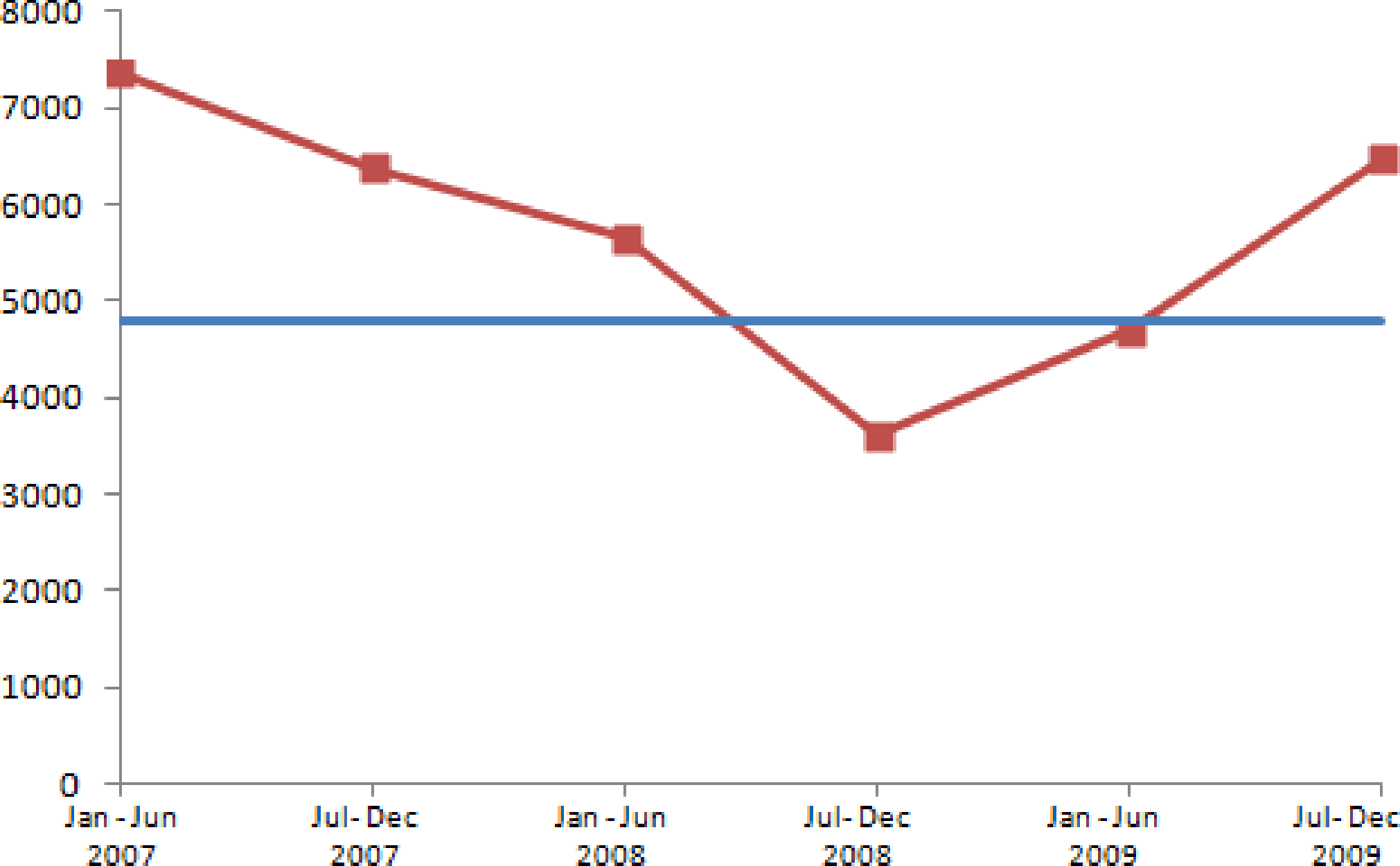
Based on the corrected statistic, the last column of this table, with significance level α = 2.5%, the half-yearly history of correlation structure instability is represented graphically in Figure 1. The dots represent half-yearly value of the corrected statistic for the i-th time window; i = 1, 2, ..., 6, and the straight line is the cut-off value for corrected Ji, i.e., the (1–α) = 97.5% quantile of chi-square distribution with degrees of freedom k = 4,560 which is equal to 4,747.17.
What we learn from Figure 1 is not only the instability of half-yearly correlation structure but also the history of its dynamics viewed from Cpooled as reference. That figure also provides us with the information that at the following time windows the correlation structure are significantly different from the reference; January–June 2007, July–December 2007, January–June 2008, and July–December 2009.
5.2. Tracking Correlation Structure Changes
The information in Figure 1 provided by the corrected statistic makes possible further investigation about to what extent the correlation structure has been changed. In this example, the correlation structure changes will be studied by comparing the pattern of the MST-based network topology issued from each time window and that issued from Cpooled. First, we compare them in terms of the power-law of degree distribution and, later on, in terms of Jaccard index.
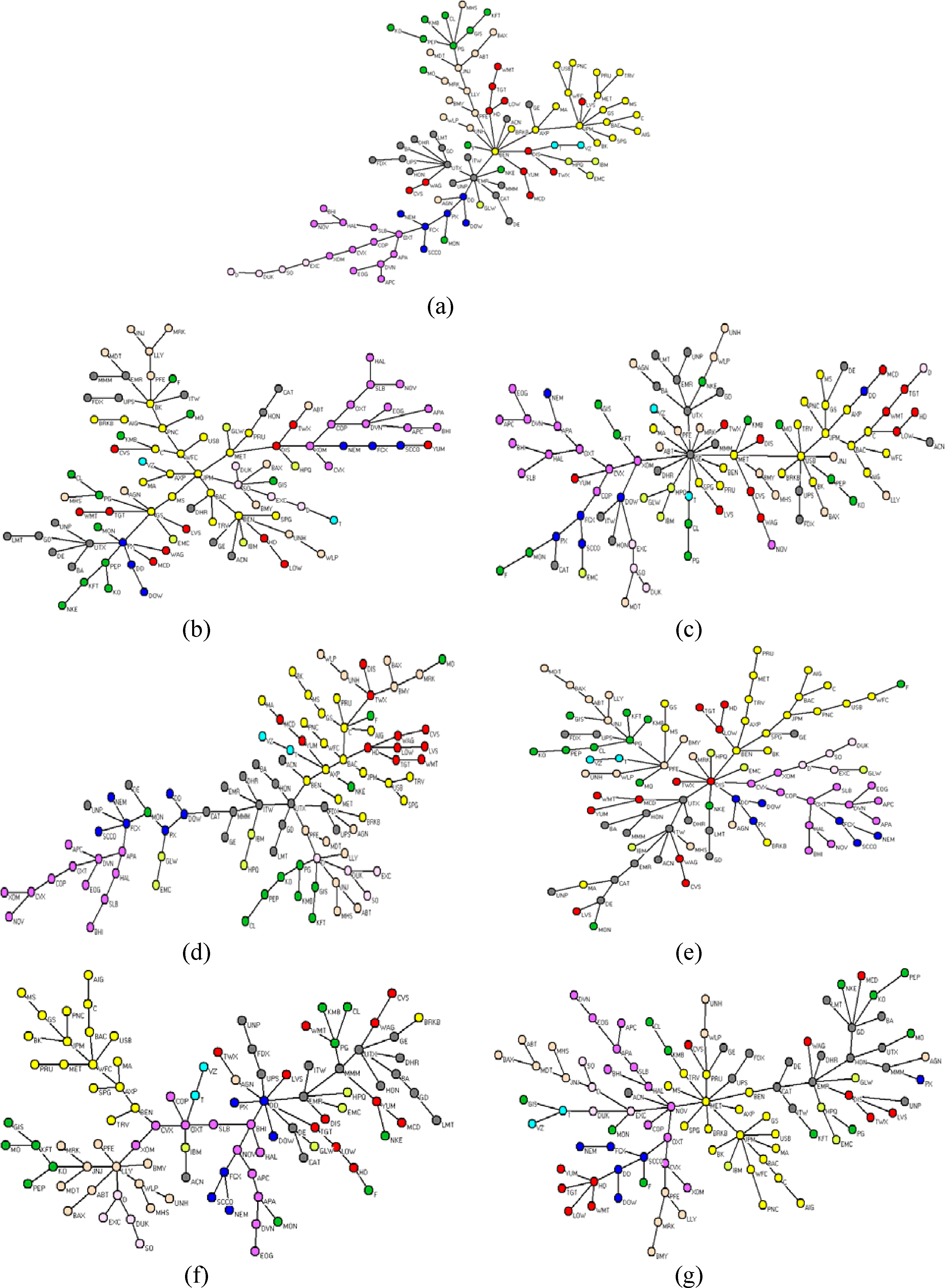
In Figure 2 we present the dynamics of correlation structure in terms of MST-based network topology among stocks [1,2,10–12]. Let us consider the pooled correlation matrix issued from all the time windows as reference. We call reference network topology in Figure 2a, the MST-based network topology of Cpooled. In Figure 2b–g we also present the network topology of the first until sixth time windows, respectively.
In that figure, the weight of the link between two stock i and j represents the distance d(i, j), related to c(i, j) in Equation (2), defined in [1,2] as:
From that figure we can investigate how degree distributions differ from that of reference correlation structure. This could lead us to investigate further the topological properties of MST-based network such as the dynamics of the most influential stocks by observing the centrality measures such as, for example, degree centrality, closeness centrality, betweenness centrality, and eigenvector centrality as usually used in networks analysis [11,12,37–40]. In what follows we focus the discussion on degree distribution.
5.2.1. Power-Law of Degree Distribution
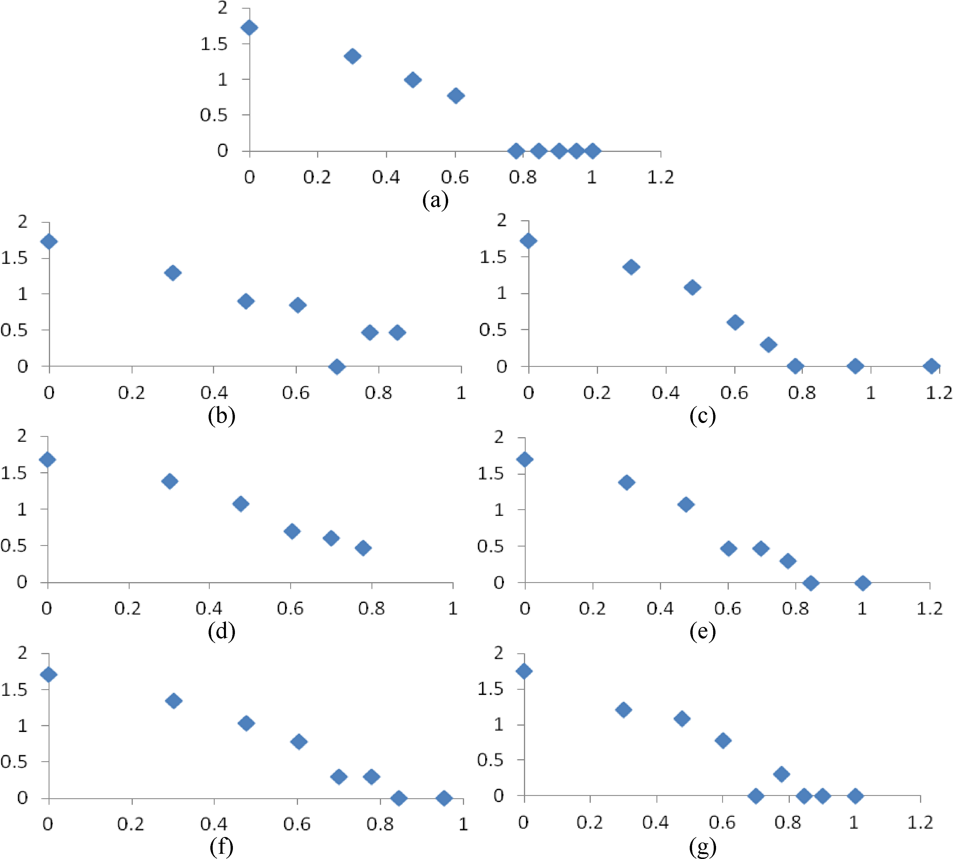
We show that, in this example, the dynamics of correlation structure in Figure 1 as monitored by the corrected Jennrich’s statistic, can nicely be explained in terms of the power-law of degree distribution for each MST in Figure 2. Graphically, in log-log scale, the degree distribution of the reference network together with that of each time window is presented in Figure 3. Horizontal and vertical axes represent log(degree) and log(degree frequency), respectively.
At a glance, this figure shows the dynamics of correlation structure in terms of the power-law of degree distribution. Specifically, let us write the power-law model P(k) = ck–γ where P(k) is the probability that a particular stock has degree k, and c and γ are constants. For each time window, the constant c and the exponent γ are given in Table 3.
From this table we learn that:
- (i)
According to Lawrence and Lawrence [41], for all time windows, the power-law model P(k) = ck–γ is reasonably fits the empirical pattern of degree distribution in Figure 3 since the mean absolute percentage errors (MAPE) is between 20% and 50% for all time windows.
- (ii)
Only the power-laws of the fourth and fifth time windows that are closer to the reference power-law related to Cpooled. These results are in-line with the result in Figure 1.
5.2.2. Jaccard Index
To track the changes of correlation structure, we can also use Jaccard similarity coefficient, also known as Jaccard index, between the reference structure Cpooled and that of each time window. This index is to measure the similarity between the MST of a particular time window and the reference MST. For the i-th time window, Jaccard index Ii, i = 1, 2, ..., 6, is defined by:
As can be seen in Table 4, this index is as nice as the degree distribution to represent the similarity between MSTi and MSTRe f. The indices for the fourth and fifth time windows are higher than the others. This is also in-line with the result given by the corrected statistic in Figure 1.
6. Concluding Remarks
Under the assumption that the time series representing stocks are governed by GBM law, Jennrich’s statistic J can be used to test the stability of correlation structure among stocks in the sense of PCC. However, if the correlation structure is unstable, J is not able to provide any information about the time windows at which the instability occurs. Therefore, J cannot tell us the dynamics of correlation structure instability along all time windows.
In this paper a correction factor is introduced in order to improve the role of Jennrich’s statistic in understanding the dynamics of correlation structure. More specifically, the corrected statistic can be used not only to test the stability of correlation structure but also to identify the particular time windows at which the correlation structure has significantly been changed.
By using the corrected statistic, a visual representation of the history of correlation structure instability along all time windows can be constructed. The information from this representation is necessary to investigate further, for example, to what extent the correlation structure in a particular time window has been changed. We have demonstrated these advantages in analyzing the dynamics of correlation structure at NYSE. According to that case of NYSE, the dynamics of correlation structur is closely related to the power-law of degree distribution. Furthermore, Jaccard index is able to quantify the similarity among two MST-based network topology.
Appendix: Proof of Property 4
Let us write:
Since the first term on the right hand side is simply , according to Theorem 2.2.2. in [31], is asymptotically distributed as k-variate normal distribution k(0,Λ) for Ti → ∞. Therefore, the distribution of can be approximated by:
Furthermore, concerning the second term on the right hand side of Equation (A1), the distribution of can be approximated by:
Therefore, the distribution of sqf (Ci,u − Cpooled,u) can be approximated by
This implies that, if Ti → ∞ for all i = 1, 2, ..., m, ; is asymptotically distributed as k(0,Λ) and consequently, we have Property 4.
Acknowledgments
The authors are very grateful to the editor and the anonymous referees whose comments and suggestions have improved the final presentation of this work. They also thank the Ministry of Higher Education and Ministry of Science, Technology and Innovation, Government of Malaysia, for financial support under Fundamental Research Grant Scheme 2013. Special thanks go to the Universiti Teknologi Malaysia for facilitating this research.
Conflicts of Interest
The authors declare no conflict of interest.
References
- Mantegna, R.N. Hierarchical structure in financial markets. Eur. Phys. J. B 1999, 11, 193–197. [Google Scholar]
- Mantegna, R.N.; Stanley, H.E. An Introduction to Econophysics: Correlation and Complexity in Finance, reprint ed.; Cambridge University Press: Cambridge, UK, 2000. [Google Scholar]
- Eom, C.; Oh, G.; Kim, S. Statistical investigation on connected structures of stock networks in a financial time series. J. Kor.Phys. Soc 2008, 53, 3837–3841. [Google Scholar]
- Rosenow, B.; Gopikrishnan, P.; Plerou, V.; Stanley, H.E. Dynamics of cross-correlations in the stock market. Physica A 2003, 324, 241–246. [Google Scholar]
- Deblauwe, F.; Le, H. Stability of Correlation between Credit and Market Risk over Different Holding Periods. Ph.D. Thesis, University of Antwerp Management School, Antwerp, Belgium. 2000. [Google Scholar]
- Ragea, V. Testing correlation stability during hectic financial markets. Financ. Mark. Portf. Manage 2003, 17, 289–380. [Google Scholar]
- Tumminello, M.; Lillo, F.; Mantegna, R.N. Correlation, hierarchies, and networks in financial markets. J. Econ. Behav. Organ 2010, 75, 40–58. [Google Scholar]
- Annaert, J.; Claes, A.G.P.; de Ceuster, M.J.K. Inter-temporal stability of the European credit spread co-movement structure. Eur. J. Financ 2006, 12, 23–32. [Google Scholar]
- Djauhari, M.A. A robust filter in stock networks analysis. Physica A 2012, 391, 5049–5057. [Google Scholar]
- Tumminello, M.; Aste, T.; Matteo, T.D.; Mantegna, R.N. A Tool for Filtering Information in Complex Systems. Proc. Natl. Acad. Sci. USA 2005, 102, 10421–10426. [Google Scholar]
- Eom, C.; Oh, G.; Kim, S. Topological properties of a minimal spanning tree in the Korean and the American stock markets. J. Kor. Phys. Soc 2007, 51, 1432–1436. [Google Scholar]
- Eom, C.; Oh, G.; Jung, W-S.; Jeong, H.; Kim, S. Topological properties of stock networks based on minimal spanning tree and random matrix theory in financial time series. Physica A 2009, 388, 900–906. [Google Scholar]
- Zhuang, R.; Hu, B.; Ye, Z. Minimal Spanning Tree for Shanghai-Shenzhen 300 Stock Index. In Evolutionary Computation, 2008, Proceedings of IEEE World Congress on Computational Intelligence, Hong Kong, China, 1–6 June 2008; pp. 1417–1424.
- Onnela, J.P.; Chakraborti, A.; Kaski, K.; Kert’esz, J.; Kanto, A. Dynamic of market correlations: Taxonomy and portfolio analysis. Phys. Rev. E 2003, 68, 056110. [Google Scholar]
- Goetzmann, W.N.; Li, L.; Rouwenhorst, K.G.J. Long-term global market correlations. J. Bus 2005, 78, 1–38. [Google Scholar]
- Larntz, K.; Perlman, M.D. A Simple Test for the Equality of Correlation Matrices; Technical Report 63; Department of Statistics, University of Washington: Seattle, WA, USA, 1985. [Google Scholar]
- Jennrich, R.I. An asymptotic chi-square test for the equality of two correlation matrices. J. Am. Stat. Assoc. 1970, 65, 904–912. [Google Scholar]
- Fischer, M. Are Correlations Constant Over Time? Application of the CC-Trigt–Test to Return Series from Different Asset Classes; SFB 649 Discussion Paper 2007-012; University of Erlangen-NĦrmberg: NĦrmberg, Germany, 2007. [Google Scholar]
- Eichholtz, P.M.A. The stability of the covariances of international property share returns. J. Real Estate Res 1995, 11, 149–158. [Google Scholar]
- Cook, W.; Mounfield, C.; Ormerod, P.; Smith, L. Eigen analysis of the stability and degree of information content in correlation matrices constructed from property time series data. Eur. Phys. J. B 2002, 27, 189–195. [Google Scholar]
- Meric, I.; Meric, G. Co-movement of European equity markets before and after the 1987 crash. Mult. Fin. J 1997, 1, 137–152. [Google Scholar]
- Lee, S.L. The Inter-temporal Stability of Real Estate Returns: An Empirical Investigation. In Proceedings of the International Real Estate Conference (ERES), Maastricht, The Netherlands, 10–13 June 1998; pp. 23–46.
- Da Costa, N, Jr; Nunes, S.; Ceretta, P.; da Silva, S. Stock market comovements revisited. Econ. Bull 2005, 7, 1–10. [Google Scholar]
- Keogh, E.; Ratanamahatana, C.A. Exact indexing of dynamic time warping. Knowl. Inf. Syst 2005, 7, 358–386. [Google Scholar]
- Podobnik, B.; Stanley, H.E. Detrended cross-correlation analysis: A new method for analyzing two nonstationary time series. Phys. Rev. Lett 2008, 100, 084102.1–084102.4. [Google Scholar]
- Wang, G-J.; Xie, C.; Chen, Y-J.; Chen, S. Statistical properties of the foreign exchange network at different time scales: Evidence from detrended cross-correlation coefficient and minimum spanning tree. Entropy 2013, 15, 1643–1662. [Google Scholar]
- Hayashi, T.; Yoshida, N. On covariance estimation of non-synchronously observed diffusion processes. Bernoulli 2005, 11, 359–379. [Google Scholar]
- Hotelling, H. The selection of variates for use in prediction, with some comments on the general problem of nuisance parameters. Ann. Math. Stat 1940, 11, 271–283. [Google Scholar]
- Lawley, D.N. On testing a set of correlation coefficients for equality. Ann. Math. Stat 1963, 34, 149–151. [Google Scholar]
- Aitkin, M.A.; Nelson, W.C.; Reinfurt, K.H. Test for correlation matrices. Biometrika 1968, 55, 327–334. [Google Scholar]
- Kollo, T.; von Rosen, D. Advanced Multivariate Statistics with Matrices; Springer: Dordrecht, The Netherlands, 2005. [Google Scholar]
- Schott, J.R. Testing the equality of correlation matrices when sample correlation matrices are dependent. J. Stat. Plan. Infer 2007, 137, 1992–1997. [Google Scholar]
- MATLAB; version 7.8.0; The MathWorks Inc: Natick, MA, USA, 2009.
- Montgomery, D.C. Introduction to Statistical Quality Control, 5th ed; John Wiley & Sons, Inc: New York, NY, USA, 2005. [Google Scholar]
- Yahoo Finance. Available online: http://finance.yahoo.com/ (accessed on 9 May 2013).
- Mason, R.L.; Young, J.C. Multivariate Statistical Process Control with Industrial Applications; ASA-SIAM: Philadelphia, PA, USA, 2002. [Google Scholar]
- Tabak, B.M.; Serra, T.R.; Cajueiro, D.O. Topological properties of stock market networks: The case of Brazil. Physica A 2010, 389, 3240–3249. [Google Scholar]
- Bonacich, P. Power and centrality: A family of measures. Am. J. Soc 1987, 92, 1170–1182. [Google Scholar]
- Micciche, S.; Bonanno, G.; Lillo, F.; Mantegna, R.N. Degree stability of minimum spanning tree of price return and volatility. Physica A 2003, 342, 66–73. [Google Scholar]
- Borgatti, S.P. Centrality and network flow. Soc. Netw 2005, 27, 55–71. [Google Scholar]
- Lawrence, K.; Lawrence, S.M. Fundamentals of Forecasting Using Excel; Industrial Press, Inc: New York, NY, USA, 2009. [Google Scholar]


| Colour | Industry Sector | Number of Stocks | |
|---|---|---|---|
 | : Thistle | Oil & Gas | 12 |
 | : Gray | Industrials | 16 |
 | : PineGreen | Consumer Goods | 11 |
 | : Cyan | Telecommunications | 2 |
 | : Yellow | Financials | 18 |
 | : LightOrange | Health Care | 12 |
 | : Red | Consumer Services | 11 |
 | : GreenYellow | Technology | 4 |
 | : Blue | Basic Materials | 6 |
 | : Pink | Utilities | 4 |
| Total number of stocks | 96 | ||
| i | Ji | Correction Factor | Corrected Ji |
|---|---|---|---|
| 1 | 6158.09 | 1.1961 | 7365.95 |
| 2 | 5306.71 | 1.2019 | 6378.34 |
| 3 | 4722.16 | 1.1981 | 5657.46 |
| 4 | 2998.50 | 1.2039 | 3609.84 |
| 5 | 3928.78 | 1.1961 | 4699.37 |
| 6 | 5376.66 | 1.2039 | 6472.88 |
| Time Window | c | γ | MAPE (%) |
|---|---|---|---|
| First | 0.5780 | 1.7485 | 48.9 |
| Second | 0.5337 | 1.7279 | 43.1 |
| Third | 0.6037 | 1.6309 | 15.3 |
| Fourth | 0.6715 | 1.9268 | 27.9 |
| Fifth | 0.7240 | 1.9895 | 26.5 |
| Sixth | 0.6505 | 1.9711 | 36.3 |
| Reference | 0.7000 | 1.9817 | 31.5 |
| Time Window | Jaccard Index |
|---|---|
| 1 | 0.284 |
| 2 | 0.203 |
| 3 | 0.250 |
| 4 | 0.338 |
| 5 | 0.310 |
| 6 | 0.203 |
© 2014 by the authors; licensee MDPI, Basel, Switzerland This article is an open access article distributed under the terms and conditions of the Creative Commons Attribution license (http://creativecommons.org/licenses/by/3.0/).
Share and Cite
Djauhari, M.A.; Gan, S.L. Dynamics of Correlation Structure in Stock Market. Entropy 2014, 16, 455-470. https://doi.org/10.3390/e16010455
Djauhari MA, Gan SL. Dynamics of Correlation Structure in Stock Market. Entropy. 2014; 16(1):455-470. https://doi.org/10.3390/e16010455
Chicago/Turabian StyleDjauhari, Maman Abdurachman, and Siew Lee Gan. 2014. "Dynamics of Correlation Structure in Stock Market" Entropy 16, no. 1: 455-470. https://doi.org/10.3390/e16010455
APA StyleDjauhari, M. A., & Gan, S. L. (2014). Dynamics of Correlation Structure in Stock Market. Entropy, 16(1), 455-470. https://doi.org/10.3390/e16010455