Article

The Measurement of Information Transmitted by a Neural Population: Promises and Challenges

1
The Fishberg Department of Neuroscience and The Friedman Brain Institute, The Icahn School of Medicine at Mount Sinai, New York, NY 10029, USA
2
Laboratory of Biophysics, The Rockefeller University, New York, NY 10065, USA
*
Author to whom correspondence should be addressed.
Entropy 2013, 15(9), 3507-3527; https://doi.org/10.3390/e15093507
Submission received: 10 May 2013 / Revised: 19 August 2013 / Accepted: 27 August 2013 / Published: 3 September 2013
(This article belongs to the Special Issue Estimating Information-Theoretic Quantities from Data)

Abstract

:
All brain functions require the coordinated activity of many neurons, and therefore there is considerable interest in estimating the amount of information that the discharge of a neural population transmits to its targets. In the past, such estimates had presented a significant challenge for populations of more than a few neurons, but we have recently described a novel method for providing such estimates for populations of essentially arbitrary size. Here, we explore the influence of some important aspects of the neuronal population discharge on such estimates. In particular, we investigate the roles of mean firing rate and of the degree and nature of correlations among neurons. The results provide constraints on the applicability of our new method and should help neuroscientists determine whether such an application is appropriate for their data.

1. Introduction

1.1. Methods for Estimating Information Content in Single Spike Trains

In the past twenty years, rapid advancements in multi-unit recording technology have created a need for analyses applicable to many neurons. While all brain functions require the coordinated activity of many neurons, neuroscience thus far has been focused primarily on the activity of single neurons [1]. These continuing advancements in both recording and imaging technologies allow the scientist to monitor an increasingly large number of neurons, and it has become desirable to estimate quantitatively the amount of information that a neural population delivers to its targets. However, the application of Shannon’s information theory [2] to neuronal discharge from more than one neuron has encountered great difficulties. At the root of the problem is the need to estimate the entropy of the discharge of many neurons from laboratory data, an estimate that is thwarted by the combinatorial explosion of the possible activity patterns. This explosion, which is severe, even for a handful of neurons, prevents the direct application of Shannon’s approach, in which entropy is defined as:
H = i p i log ( p i )
where each p i is the probability of a particular pattern of spike-events. The reason for this failure is that laboratory data sample the space of possible activity patterns rather sparsely, and this sparsity undermines our confidence in the knowledge of the underlying distribution, a knowledge that is critical for the determination of the probabilities in Equation (1). This difficulty is referred to in the literature as the small sample bias, and several ad hoc counter-measures have been proposed, although those have been limited to a small handful of neurons [3,4,5].
The primary purpose of this paper is to test the robustness of our recently developed Fourier-based method [6,7] that in common, reasonable circumstances bypasses the small sample bias when applied to simulated or real data. We first describe a general linear modeling simulation [8,9] that we used to generate simulated data, and, then, present a series of tests, each of which is designed to pit the method against a specific set of parameters; we present the tests sequentially along with their results.

1.2. The Fourier Method

In general, and particularly for signals as complex as those found in the brain, far fewer data points are required to describe a probability distribution whose shape is known a priori, as in the case of a Gaussian distribution, than for distributions of arbitrary shape. Well-established methods, such as the Direct Method [10], require large data sets, because those arbitrary distributions must be well-described before information can be estimated. The Fourier Method exploits the fact that the entropy of a Gaussian-distributed process can be analytically calculated from its variance:
H ( x ) = 1 2 log ( 2 π e σ 2 ) .
Our method further exploits the fact that stochastic variables that lose correlation with their past history yield Fourier coefficients that follow a Gaussian distribution [6], allowing us to directly apply this analytic measure of entropy.

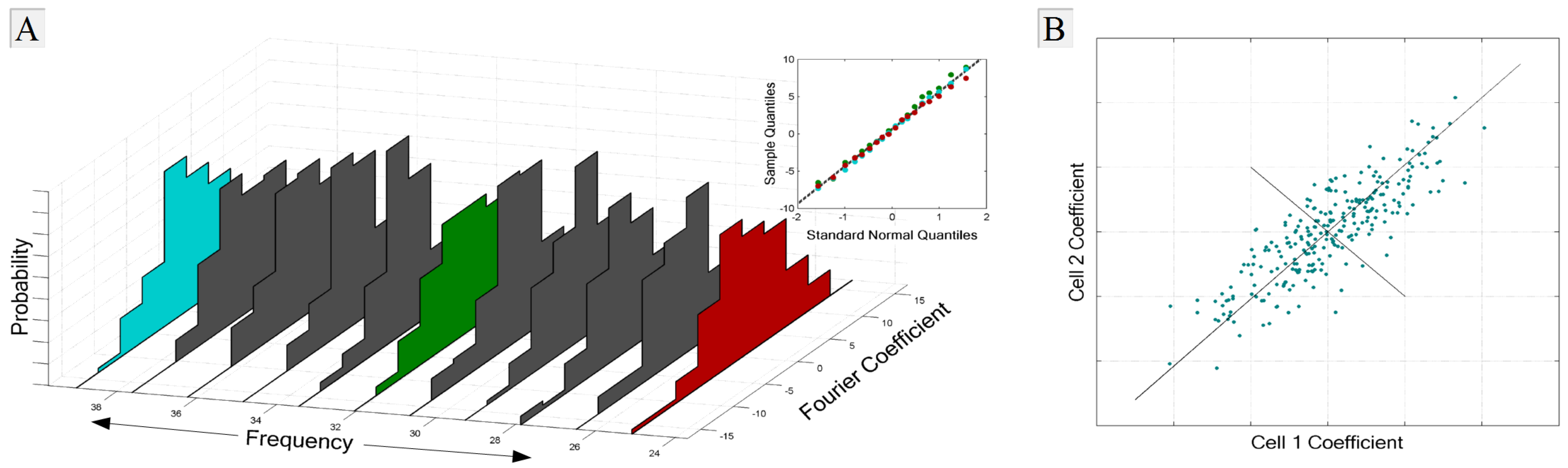
1.2.1. Representing Neural Signals in the Frequency Domain

Visual neuroscientists are concerned with the mapping of visual scenes to patterns of neural activity. Since the primary mechanism by which many neurons communicate information is the action potential, a neural activity pattern can be described as a list of spike times, t n , which we call a spike train, and is commonly expressed as a sequence of δ-functions:
u ( t ) = n = 1 N δ ( t t n )
where t n is the time of the nth spike. We may now represent this signal as the weighted sum of a set of conventional orthonormal basis functions consisting of cosines and sines:
u ( t ) = 1 2 a 0 + m = 1 a m cos 2 π m T t + b m sin 2 π m T t
with the weighting coefficients evaluated directly from the data by:
a m = 2 T 0 T u ( t ) cos 2 π m T t d t and b m = 2 T 0 T u ( t ) sin 2 π m T t d t
When the statistics of a neuron are stationary, as required for this method, the variance of the mean rate across trials is small, and therefore, spike trains of sufficiently long duration carry very little information in the mean value of the signal. The initial term, a 0 , can thus be discarded. Additionally, when the input signal, u ( t ) , is represented by a series of δ functions at times t n , u ( t ) is zero for all t { t n } , and the weighting coefficients in Equation (5) can be directly expressed in terms of the spike times, e.g.:
a m = 2 T n = 1 N cos ( 2 π m T t n )
Through this process, we convert a spike train to a series of cosine and sine coefficient pairs that advance in frequency in increments of 1 / T . While a full description of the original signal requires that we measure these coefficients to infinite frequencies, in practice, we can determine a natural cutoff frequency above which no further information is carried. The determination of this cutoff is described in Section 1.2.4.

1.2.2. The Fast Fourier Transform

An alternative representation, in which spike trains are discretized into bins of length δ t , such that a one represents a spike and a zero represents the absence of a spike, allows for the application of the Fast Fourier Transform, which in modern computer systems, is highly optimized and provides significant speed improvements over implementations of the classical Fourier system described above.

1.2.3. Entropy in the Neural Signal

If we generate multiple realizations (trials) of the neural signal in response to a particular class of stimuli, we build, at each frequency bandwidth, ω, distributions of cosine and sine coefficients, P cos ( ω ) and P sin ( ω ) . As is discussed in [6], these distributions are Gaussian, and their respective variances, σ cos 2 ( ω ) and σ sin 2 ( ω ) , are used as in Equation (2) to evaluate the entropy of each distribution; the entropies of the cosine and sine coefficients together sum to form the entropy of the process at a given frequency bandwidth, with the entropy of the complete signal being the sum of the entropies contained in all bandwidths:
H = ω H ( P cos ( ω ) ) + H ( P sin ( ω ) ) .
The entropies, H ( P cos ) and H ( P sin ) , are calculated from the Gaussian-distributed Fourier coefficients across trials, using Equation (1):
H = ω ( 1 2 log 2 e σ cos 2 ( ω ) ) + ( 1 2 log 2 e σ sin 2 ( ω ) )
Figure 1A shows histograms of several cosine component distributions from data taken from the lateral geniculate nucleus (LGN) of Macaca fascicularis using 128 trials. Q-Qplots at three select frequencies (indicated by red, green and blue) are displayed in the inset; the linearity of these plots demonstrates that typical electrophysiological data do indeed follow a Gaussian distribution. The robustness of this Gaussian assumption is further tested in Section 3.3.1.
Figure 1. Fourier coefficient variance and covariance. (A) Fourier cosine coefficients from the monkey lateral geniculate nucleus (LGN) are collected and form Gaussian distributions at each frequency, represented by histograms. The inset shows Q-Q plots of the three highlighted distributions; the linearity of the sample points indicates Gaussianity. The variance of each of these distributions is used to calculate the entropy at each frequency. (B) Simulated data to illustrate the multivariate case. The variance along the principal axes (black) is determined by the covariance matrix of the coefficients and informs us of the information conveyed by the population.
Entropy 15 03507 g001
The process of extending the Fourier entropy calculation to multiple neurons becomes intuitive from inspection of the two-neuron example in Figure 1B, which shows a two-dimensional plot of the cosine coefficients of each neuron at a chosen frequency, with one (simulated) data sample per trial. Each neuron’s coefficients form a one-dimensional Gaussian distribution, whose variance provides us with an estimate of that neuron’s entropy alone at that particular frequency (Equation (2)). When the coefficients for the two neurons are plotted against each other, correlations between neurons induce correlations in their respective coefficients. In this case, the output from one neuron informs us to some degree of the output of the other, the result being a reduction in entropy associated with their joint distribution. This reduction is taken into account when the coefficients are expressed along their more compact Principal Component axes, shown in black; in this new coordinate system, information conveyed about the structure of the correlations between the neurons, rather than information about the stimulus, is discarded, and the joint distribution entropy, which we call the group entropy, H ( G ) , is revealed [11]. The entropy of this multivariate Gaussian distribution is readily calculated by replacing the variance, σ 2 , in the single-neuron case with the covariance matrix of the multiple neurons’ coefficients and is the sum of the entropies along these principal axes. We call the difference between the group entropy and the sum total of the individual neurons’ entropies the redundancy, which we express as a proportion of the total entropy, summed over all frequencies:
R = 1 H ( G ) H ( C )
where:
H ( C ) = c C H ( c )
where H ( G ) is the group entropy rate that conveys the signal entropy, taking correlations into account, and H ( C ) is the sum of the individual entropy contributions of each neuron, which ignores correlations. In the special case in which H ( G ) > H ( C ) , R becomes negative, and we have synergy; a population code. This method generalizes to a large number of neurons and is described in detail in our previous publications [6,7].

1.2.4. Noise and Signal Entropies

Fluctuations in spike times due to noise produce additional entropy, the magnitude of which is limited only by the precision at which spike times are measured. This entropy due to noise, H N , must be subtracted from the total entropy, H T , in order to measure the information in the signal:
I = H T H N .
Experimentally, one may measure the imprecision of a system by observing the variability of its responses to repeated, identical inputs. Our simulations and experiments apply this technique through the use of a repeat-unique paradigm. In such a paradigm, the total entropy is calculated from a rich variety of unique signals to which the neuron responds noisily, while the entropy due to this noise alone is calculated from responses to identical, repeated patterns of input. Thus, the variation in the response of a neuron to a repeated stimulus provides a measure of its noise. Example stimuli are shown in Figure 2B, first with the repeated stimuli, all identical, plotted in red, and, then, followed by unique stimuli, plotted in blue. The responses of a neuron (simulated or real) to unique and repeat trials are represented with a raster plot, with each row representing a separate trial and hash-marks indicating spike times (Figure 2C).
Figure 2. Simulated neuronal response to the repeat-unique stimulation paradigm. (A) General linear modeling (GLM) flow diagram, adapted with permission from Macmillan Publishers Ltd: Nature [12], ©2008. (B) A subset of the trials of a typical stimulus are displayed. Repeat stimuli (red) are all identical, whereas unique stimuli (blue) are each different from all others. (C) Raster plot of the responses of a simulated neuron to repeat and unique stimuli. Each row of the raster corresponds to a single trial, seen on the left. Responses to 128 trials are displayed in the raster; because repeat stimuli are all identical, the neuron produces similar spike trains (red spikes), evidenced by the appearance of vertical stripes. The response of the neuron to unique stimuli is different with each trial, and therefore, no stripes appear. (D, top) The entropy rate calculated in response to the repeated stimuli (red) is subtracted from the entropy rate calculated in response to the unique stimuli (blue); the difference between the entropies (shaded area) is the signal information rate. The integral of this entropy difference over frequency is dimensional information times frequency or equivalently bits per second. (D, bottom) The information rate is plotted as a cumulative sum across frequencies; the plot levels off with a near-zero slope at frequencies above which signal information is zero.
Entropy 15 03507 g002

1.3. Overview

In simulation, we are not subjected to the limitations of experiment. Consequently, the accuracy of our calculation increases with the amount and quality of available data, over which we have direct control. Here, we explore the performance of the Fourier Method when applied to various kinds of neuronal populations and discharge patterns. In particular, we wish to establish the constraints imposed on the method by some important aspects of the neuronal discharge, such as the mean rate and variability of the discharge, as well as the degree and nature of the interactions (correlations) among the neurons in the population.
We begin with simple information profiles of neurons with a wide range of firing rates in response to a stimulus of increasing frequency. We then address the basic question of data quantity—what is the minimum recording length required to generate valid information estimates, and how does this requirement depend on the firing rates of the neurons? Following this, a series of potentially confounding experimental factors are introduced: firing rate non-stationarity, spike-to-neuron assignment errors and biased estimates of noise entropy. We conclude with a study of the effects of scaling the method to multiple neurons and demonstrate its strength in dealing with very large populations of cells.

2. Methods

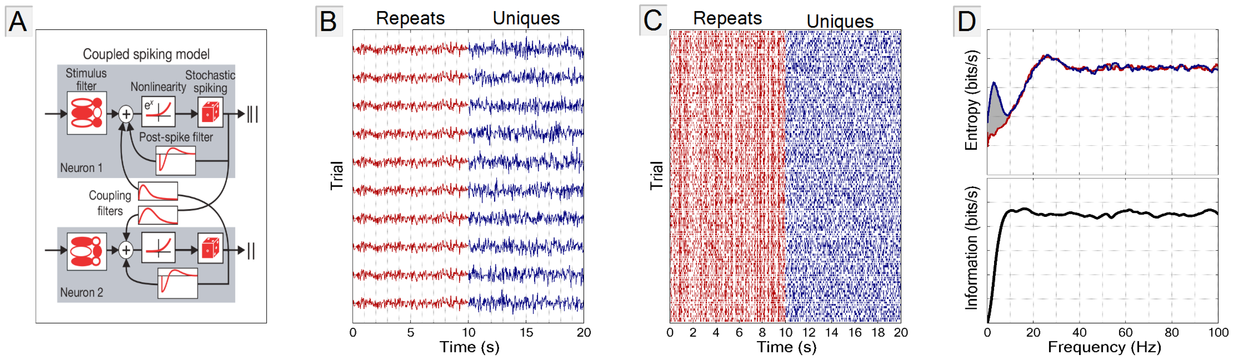
2.1. The GLM Simulation

To explore the performance of our method, it is appropriate to use simulated data sets, where we have control over the relevant parameters. Among many possible simulation frameworks, we chose the general linear modeling (GLM) approach described by [8,9], which was effectively used by these authors to model populations of primate retinal ganglion cells [12]. This framework allows us to control important features of the dynamics of individual neurons, as well as to control the strength and dynamics of the interactions among the simulated neurons in the population. A detailed description of the model can be found in [8,9,12] and is illustrated in Figure 2A [12]. An input stimulus is first passed through the stimulus filter, designed to mimic ON retinal ganglion cells that maximally respond to increases in light intensity. A nonlinearity is applied to the filtered output, and a stochastic spiking model produces stimulus-dependent spikes. Following a spike, a post-spike filter is applied to the input, generating a refractory period. If multiple neurons are simulated, additional post-spike coupling filters are applied, which allow neurons to influence each other. The coupling filters can be unique for each pair of neurons, allowing for a variety of connection types and strengths within a single network.

2.2. Stimulus

Figure 2A includes a stimulus filter designed to selectively emphasize stimuli of a particular spatial pattern, and while the GLM simulation is capable of handling a variety of complex, spatially-rich stimuli, we first chose to drive each neuron with a one-dimensional stimulus, in order to reduce the number of input parameters. The stimulus filter carries a time-component, as well, allowing one to mimic some of the properties of neurons found in the brain. Our choice of one-dimensional stimulus and a spatial filter effectively models a full-field stimulus driving a retinal ganglion cell whose maximal response arises from a sharp increase in stimulus intensity. The stimulus provided to our simulated neurons consists of Gaussian-distributed random intensity values, each lasting for a brief interval, whose mean value determines the mean firing rate of the cell. An offset is applied to simulate neurons of any desired mean firing rate. The interval during which each stimulus value is shown determines the stimulus sampling rate, which is a parameter in our simulation. Figure 2B shows the inputs of ten sample trials of Gaussian inputs presented at 25 Hz.

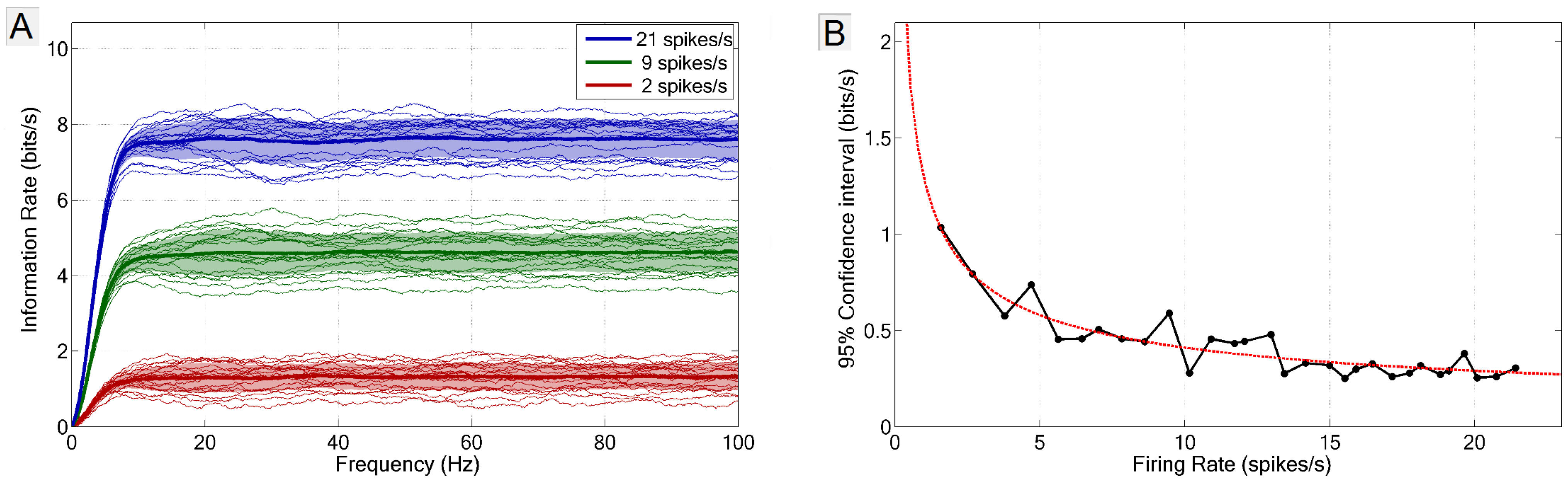
2.3. Frequency vs. Information Plots

Typical plots of entropy and information as a function of temporal frequency are displayed in Figure 2D. The difference between the entropy calculated from the unique runs (blue) and repeated runs (red) is the signal information (shaded gray area). The bottom panel in Figure 2D displays a cumulative plot of signal information, which levels off at frequencies above which no signal information is transmitted.

2.4. Measurement of Error and Confidence

Many of the simulations that follow require a measure of the relative quality of the information estimation. Given that the sources of our data here are (simulated) neurons, a calculation of error requires a comparison between a measured and a “true” information rate. Our calculations provide estimates with units of bits per second, and in situations where the estimation may be improved by simply increasing the quantity of data, we can declare our true information rate to be that rate estimated from a large quantity of data. Our error is thus defined to be the absolute value of the difference between the measured rate and the true rate, divided by the true rate and represented as a percentage. Thus, our error is bounded by zero below and is unbounded above. We calculate this confidence interval by generating multiple instances of the true rate and determining the standard deviation of such results.
Figure 3 displays the intrinsic variability of neurons with various firing rates responding to a 25 Hz stimulus, as described in Section 2.2. Panel A displays the spread of information for neurons of three different firing rates, with mean values plotted as solid lines. The resulting spread is used to define the 95% confidence interval (1.96 standard deviations), which is shown in Panel B for a more densely sampled choice of firing rates, and fit with a function of the form, a x b . Notably, the reliability of the information estimate increases with the firing rate.
Figure 3. Intrinsic variability of neural responses. (A) Twenty instances of cumulative information rates from three single neurons, with firing rates of 21, 7 and 2 spikes/s. (B) Standard deviations of information rates from twenty neurons, three of which are derived from the neurons in the left panel, fitted with the function, ( y = 1 . 29 x 0 . 497 ). The fitted curve is used to describe the 95% confidence interval of the information estimation.
Entropy 15 03507 g003

3. Results

3.1. Comparison with the Direct Method

We begin with a brief comparison of our method with a well-known standard of information estimation: the Direct Method [10]. The Direct Method is named for its simplistic approach: spike trains are discretized into binary vectors of length Δ τ and subdivided into words of window length L, with the resulting distribution of words subjected to Shannon’s formula in Equation (1); the entropy of the words of window length T and bin width Δ τ is thus:
H ( T ; Δ τ ) = i p i log 2 ( p i ) .
Calculation of the true information rate requires that we calculate this sum to the limit as L and Δ τ 0 . The small sample bias precludes estimation of even modest word length L, and therefore, an extrapolation towards the infinite data limit is required [10].
Figure 4A compares the Direct Method with the Fourier Method. We applied both methods to the discharge of 25 simulated neurons with firing rates ranging from 5 spikes/s to 30 spikes/s, ensuring a range of information rates. For this comparison, we provided 4,096 trials of 30 s each in order to ensure that the Direct Method was not limited by the sample size; this corresponds to approximately 68 hours of recording for each choice of firing rate and sensitivity. The results show that the two methods produce similar results. Figure 4B demonstrates the increase in information rate errors as the number of trials decreases, with the inverse of the number of trials shown on the abscissa. While the rate error resulting from use of the Direct Method increases drastically as the number of trials decreases, the Fourier Method remains robust even in the face of a small sample size. Approximately one tenth of the quantity of data required by the Direct Method is needed for the Fourier method to achieve a comparably reliable estimate. Because of the far smaller response to noise in the Fourier method, the vertical scatter in Figure 4A can be regarded as an indication of the accuracy limitations in the Direct Method.
Figure 4. Comparison with the Direct Method. (A) Spike trains from 25 simulated neurons of varying firing rates and input sensitivities were subjected to both the Fourier and Direct methods of information measurement, using 4,096 trials of 30 s each to ensure enough data. (B) Rate errors expressed as a function of the inverse of the number of trials. The rate errors produced by the Fourier method remain small compared to those produced by the Direct Method as the number of trials decreases.
Entropy 15 03507 g004

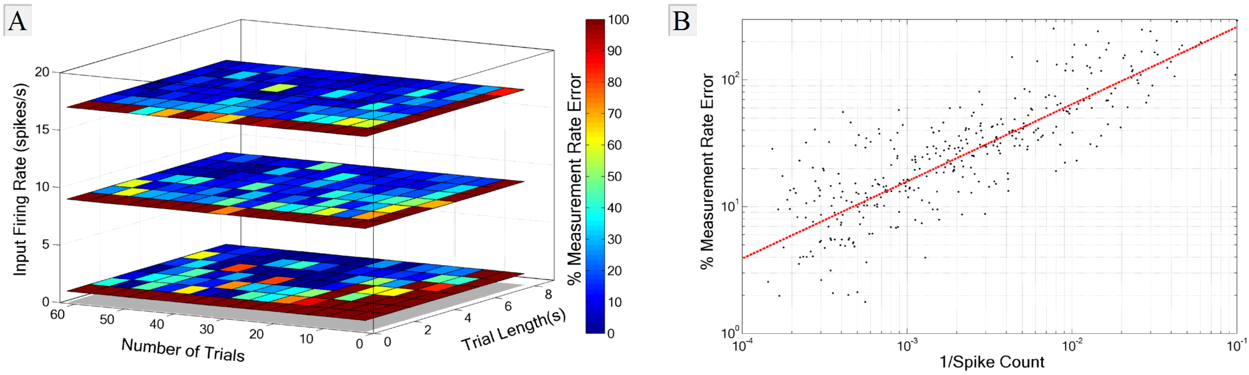
3.2. Experimental Requirements

A data set extracted from an experiment is but a small sample of the total neural activity, acquired during a limited time period. An important question arises, therefore: how much data does one need to properly estimate information rates? Statistical inference relies on the ability of a limited sample to represent features of a population; the sample must therefore be a faithful representative of the population and be sufficiently informative for the scientist to extract the relevant features. How much data do we need to measure information in the discharge of a neuronal population?
The range of properties of individual neurons encountered in the brain is large, even among neurons confined to individual nuclei. In our simulation, we chose a set of model parameters that covers a typical range of neuronal properties encountered in the laboratory. We address the issue of experimental requirements—how much data one needs to measure information—by an iterative process of the reduction of sample size until the error renders the method unusable. We have explored three independent parameters (Figure 5) in this investigation: mean firing rate, trial length and number of trials, all of which contribute to the total number of spikes recorded. For each input firing rate, we generated a reference measurement using 2,048 trials, each of them 10 s in length, which we deemed sufficient as a basis for comparison. While the information rate of a neuron is not simply tied to its mean firing rate, our wish to gain valid statistical measures requires that we have enough spikes to accurately characterize the distribution of Fourier coefficients at any relevant frequency.
Figure 5. Experimental requirements for information calculation. In this simulation, trial length and number of trials were altered independently. Information rates were calculated and compared to a reference information rate, with the difference expressed as a percentage deviation from the true (reference) rate. (A) Rate errors are displayed as a function of both the number of trials and trial length, with red indicating parameter choices that produced high rate errors. Slices represent the choice of input firing rate into the model. (B) Rate error plotted as a function of the total spike count, which is itself dependent on trial length, number of trials and firing rate. Rate errors in the right panel were fitted with a function of the form, E = a x b .
Entropy 15 03507 g005
The results of the simulation can be seen in Figure 5. The error is represented as a percentage deviation of the reference simulation from the 95% confidence interval of the information rate measurement. The independent contributions of trial number and trial length can be seen along the columns and rows of Figure 5A. Not surprisingly, rate errors increase significantly as the amount of data is reduced. Slices indicate the three input firing rates of one, nine and 17 spikes/s, and each data point represents the mean rate error of five runs with identical input. As firing rate increases, the restrictions on trial length and number of trials decrease. Figure 5B shows the error in information rate purely as a function of the inverse of the number of spikes. The total spike count itself, while not entirely indicative of the ability of the method to accurately estimate information, provides a good rough estimate for the amount of data required to produce low-error estimates. The dotted red line was fitted to the data by the function, y = 1063 x 0 . 609 ; the 5% error level occurs at approximately 6,636 spikes; for a typical cortical neuron that fires at five spikes/s, an experimentalist would thus require approximately 22 minutes of data.

3.3. Recording Pitfalls

Recording stability is often imperfect in the laboratory: varying levels of anesthesia, electrode drift, attentional effects and interference all affect the recording. These effects can manifest themselves in several ways, including:
  • Firing non-stationarity
  • Spike-to-neuron assignment errors during spike sorting
  • Biased estimation of noise entropy
To assess the impact of these pitfalls, we have created the three simulations described below.

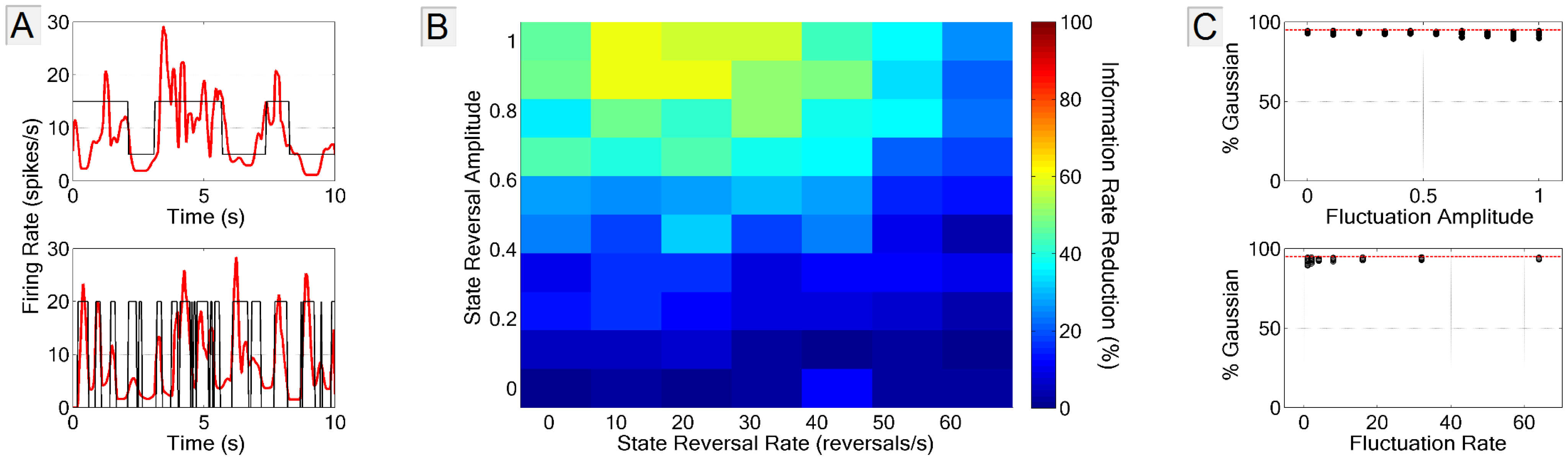
3.3.1. Firing Rate Non-Stationarity

Electrophysiological experiments are often performed on animals under anesthesia, during which brain activity assumes a state of slow-wave oscillatory behavior, commonly associated with sleep. In unanesthetized animals, the high-conductance neuronal states found in thalamocortical and cortical systems during wakefulness give rise to increased neuronal activation, accompanied by increased sensitivity to stimuli, more variable spiking patterns, greater desynchronization [13] and a shortened membrane time constant, a consequence of which is higher temporal precision [14]. The phasic activity observed during anesthesia and the transitions between wakefulness and sleep due to fluctuations in the metabolism of anesthetics can both contribute to changes in the firing rates of neurons that are not necessarily stimulus-induced. In addition, many neurons in the brain have been found to exhibit discharge patterns indicative of high and low firing states. These Up and Down states can result from either intrinsic properties of the membrane or from network-related activity and have been observed most prominently in cortical pyramidal cells and striatal spiny neurons, with stable Down states consisting of periods of low activity, and either stable or meta-stable Up states, where the neuron enters a heightened state of activity (see [15] for a review of the subject). Similarly, neurons of the lateral geniculate nucleus are known to display tonic and burst firing patterns [16] that may play a role in the transmission of visual information [17]. Regardless of the mechanism, it is important to determine the effect of such instability on the calculation of information.
A primary concern is that a neuron exhibiting multiple modes of activity might violate the requirements of the Central Limit Theorem and produce non-Gaussian Fourier coefficient distributions. We address this potential concern by simulating Up and Down states in neurons, with two variable parameters: the difference between firing rates in the two states (reversal amplitude) and the average rate of fluctuation between the two states (reversal rate). All neurons in this simulation had a mean firing rate of 15 spikes/s; two sample neurons can be seen in Figure 6A with different reversal amplitudes and rates. To test the possibility that the normality assumption of Fourier coefficients is violated in neurons exhibiting multiple modes of firing, we subjected the coefficient distributions at each frequency used in the information calculation to the Shapiro-Wilk test for non-normality ( N = 4 , 000 distributions; α = 0 . 05 ) and display the results as a percentage of the number of distributions that did not violate the Gaussian property at the 5% significance level.
Figure 6. Effects of firing rate instability. Neurons with bimodal firing statistics were simulated, switching between Up and Down states throughout each trial. The firing rate difference between Up and Down states is represented as a proportion of the mean firing rate and the average duration of each state by its reciprocal in Hz. (A) Firing rates of two sample neurons are plotted in red, each with a mean firing of 10 spikes/s. The top neuron oscillates between five and 15 spikes/s (reversal amplitude = 0.5), with a mean fluctuation rate of 0 . 5 Hz . The bottom neuron oscillates between zero and 20 spikes/s (reversal amplitude = 1.0), with a mean fluctuation rate of 3 Hz. (B) Heat map illustrating the effect of state fluctuation on information rates. All neurons had mean firing rates of 15 spikes/s; information decreased with reversal amplitude, with the effects of the decrease being partially mitigated by increases in reversal rate. (C) The fraction of of Fourier coefficients distributions that were Gaussian plotted against reversal amplitude and reversal rate. Fourier coefficient distributions at each frequency were subjected to the Shapiro-Wilk test for non-normality at the 5% significance level (dashed red line).
Entropy 15 03507 g006
Figure 6B shows the dependence of the information estimation on both the state reversal rate and the reversal amplitude. Reversal amplitude had a largely negative effect on information rates, whereas reversal rate had the opposite effect. This mitigating effect results from a trend toward homogeneity of the firing rate as the reversal rate increases. Note that values are not reported as rate errors, but as information rate reductions; this is because the observed decreases in information are due not to failure of the method, but because properties of the simulated neuron itself affect the information rates. Indeed, Figure 6C shows that the distributions remained Gaussian, even in the case of prominent changes in a neuron’s firing state and pattern. Clearly, the non-stationarity of firing patterns did not violate the Gaussian requirement, and our method is applicable under such circumstances. We do, however, stress the importance of testing for Gaussianity. While the data provided in our experimental paradigm generate signals with necessarily short autocorrelation times, other experiments may result in violation of the Gaussianity assumption.

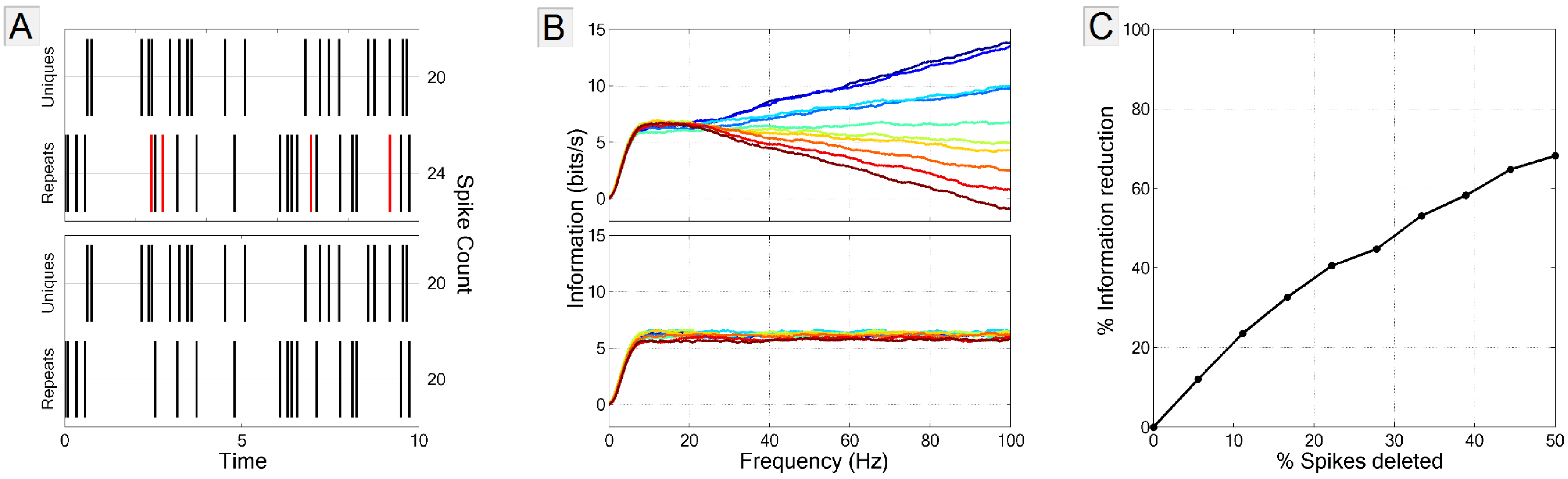
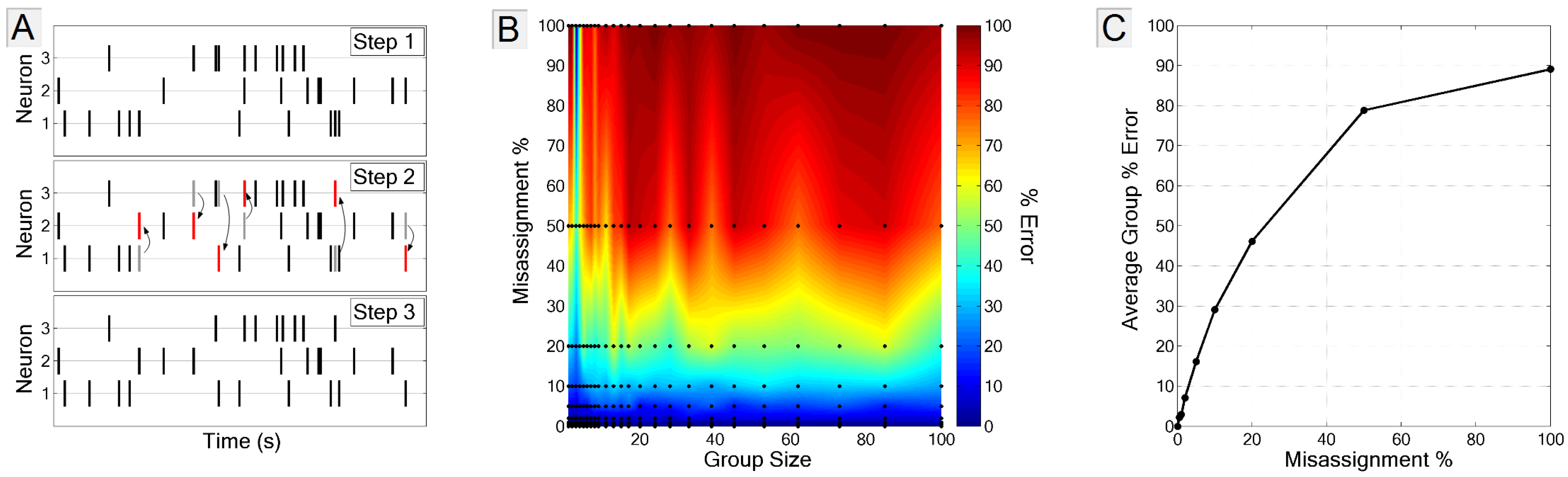
3.3.2. Spike-Neuron Misassignment

Electrophysiologists are familiar with the challenging process of spike sorting that is routinely encountered in the context of multi-electrode recordings, in which the activity of many neurons is recorded. Voltage recordings from such experiments provide estimations of the number of neurons and the timing of spikes associated with each neuron. While the probabilistic methods that are utilized in spike sorting often result in reliable assignments of spikes to their respective neurons, they still rely on incomplete knowledge of the environment; the misassignment, over-assignment or under-assignment of spikes to neurons is sometimes unavoidable. In sub-optimal recordings, spike sorting is limited by the signal-to-noise ratio, and unidentified action potentials muddle the knowledge of the true time course of a neuron’s activity. To study the impact of spike misassignment on information rate, we ran a simulation in which a percentage of spikes from each neuron were distributed equally and at random to the other neurons (Figure 7A). Rate errors were represented as the percent deviation from the true rate, in which no spikes were misassigned; a value of 0% thus indicates no misassignment and a value of 100% means that every spike from each neuron is evenly assigned to the other neurons. In this simulation, neurons were driven by separate, uncorrelated stimuli to remove correlations between neurons induced by the stimulus. We progressively increased the group size to determine whether the problem of misidentified spikes is exacerbated by a greater number of neurons. Twenty four group sizes and nine misassignment percentages were chosen, both along a logarithmic scale, and information rate errors calculated for these 24 × 9 conditions and linearly interpolated along both dimensions.
Figure 7. Effect of spike-neuron misassignment on information rate. (A) The spike neuron misassignment procedure follows three steps: (1) spike rasters for individual neurons are generated; (2) a percentage of spikes from each neuron, highlighted in red, are selected at random; (3) the selected spikes are evenly distributed to the other neurons. (B) Average rate errors are expressed as a function of both the number of neurons and of the misassignment percentage. Sampled points are displayed as black dots, and the values are interpolated to create a smooth heat map. (C) Average rate errors, averaged across group sizes, with the special case of two neurons excluded.
Entropy 15 03507 g007
Figure 7B demonstrates the impact of spike misassignment on information rate. The 24 × 9 conditions in which the impact of spike misassignment was calculated can be seen in Figure 7C, and the sampled values are indicated by the black dots; these data were interpolated to produce the smooth heat map. As expected, complete misassignment results in a nearly complete destruction of signal information, with the exception of the two-cell case, in which a full 100% misassignment of spikes is equivalent to swapping the two neurons and can be observed by the vertical blue line centered at group size = 2 . Group size plays little role in calculating the impact of misassignment, and the values averaged across group sizes, with the two-neuron cases excluded, are shown in Figure 7C. A misassignment of as little as 10% of spikes can degrade information calculations by up to 30%, underlining the importance of careful and proper spike sorting.
It is important to note that the neurons used in this simulation have identical tuning properties, and therefore, the stimulus patterns about which the neurons are reporting will be correlated to some extent. The result is that these neurons will report on similar features of the stimulus and, therefore, will be redundant. Consequently, a complete misassignment of spikes to neurons still yields a low information rate, and therefore, the rate error approaches, but does not quite reach, complete error.

3.3.3. Biased Estimate of Noise Entropy

For a proper measure of signal information, it is crucial to estimate accurately the noise entropy of the system. Because signal information is the difference between the unique and repeat entropies, any situation in which the noise (repeat) entropy is miscalculated will lead to an invalid estimate of signal information. It is therefore important that the repeated stimulus be a faithful representative of the unique stimulus ensemble. An atypical repeat stimulus can be detected from the resulting spike trains and the bias corrected to the extent possible, but it is clearly in the interest of the experimenter to reduce the level of post-hoc statistical adjustments to a minimum.
A simple, but crude, indication of a statistically atypical repeat stimulus is the difference in the number of spikes produced in response to the unique and repeat stimulus sets. An atypical repeat stimulus may generate a neuronal response that contains fewer or more spikes than those produced on average by the unique stimuli. The resulting effect on the cumulative information plot is easily recognizable: as one proceeds toward high frequency, information accumulates at a constant rate, with a steady increase or decrease in the cumulative plot at frequencies past the signal frequency cutoff. The cosine and sine terms of a Fourier coefficient together define a vector on the unit circle of the complex plane. At sufficiently high frequencies, at which no two consecutive impulses are correlated, the phase becomes a uniformly distributed random variable, and the complex Fourier coefficient is the result of a two-dimensional random walk of unit-length steps, corresponding to each spike, in random directions. The two-dimensional variance of these coefficients across trials at these high frequencies therefore depends only on the number of spikes. Ideally, a collection of coefficients at such frequencies from repeats should have the same variance as coefficients from uniques, yet differences in the number of spikes create an inequality in these variances. The two entropies, which depend on these variances, are consequently unequal, and a resulting negative or positive information content accumulates. A simple and effective method of resolving the spike-count discrepancy error is the random deletion of spikes, until the repeat and unique sets contain an equal number of spikes (Figure 8A). The extent to which this affects the information calculation is dependent on the number of spikes deleted, but in most cases, the result is a minimal change at the relevant frequencies. The concern is the accumulation of information at frequencies beyond the signal cutoff frequency, which, in the case where responses to repeats and uniques have unequal spike counts, is determined entirely by the arbitrary frequency at which one stops the calculation.
Figure 8. Spike Deletion Procedure. (A) Deletion of randomly selected spikes (shown in red) from the spike train with more spikes abolishes high-frequency information miscalculation. (B, top) Information accumulates (cool colors) at high frequencies in the case where the number of unique spikes exceeds the number of repeat spikes, and declines (warm colors) when the repeat set is larger. (bottom) After the spike deletion procedure, information accumulation trends are abolished. (C) The percentage of information reduced as a function of the percentage of spikes deleted in both the repeat and unique sets.
Entropy 15 03507 g008
Figure 8B shows results from ten sample simulated neurons, whose firing rates in response to the unique stimuli were systematically adjusted from 14–16 spikes/s and paired with a repeat stimulus rate of 15 spikes/s. When the repeat spike count exceeds the unique spike count, a negative trend occurs (warm-color curves), with positive trends (cool-color curves) occurring when responses to the uniques exceed those elicited by the repeats. Application of the spike deletion procedure effectively abolishes the information accumulation problem (Figure 8B). The resulting information rates form a distribution around the true information rates with a standard deviation of 0.2 bits/s, which corresponds to a spread of approximately 3%.
To gauge the extent to which information is affected by spike deletion, we ran a simulation (Figure 8C) that illustrates the relationship between the number of spikes and the percentage reduction in information. Note, however, that the right panel of Figure 8 does not indicate spike-count discrepancies, but rather, percentage deletion from both uniques and repeats in tandem; in the case where discrepancies between unique and repeat spike counts exist in the laboratory, the number of spikes deleted will be roughly half of those deleted in our simulation, because such a discrepancy necessitates deletion from only one of the two (unique or repeat) sets. To get a sense of the number of spikes that must be deleted on average, we turned to a recent recording of neurons in the lateral geniculate nucleus of Macaca fascicularis. The spikes from these LGN cells were sorted using in-house software, and neurons with firing rates less than 0.5 spikes/s were discarded. Of the 25 resulting neurons, the average spike count discrepancy between unique and repeat sets was 1.9% with a standard deviation of ± 1 . 4 % ; these values correspond to 0.95% ± 0.7% of the total spikes that must be deleted to equalize the two spike counts. Following the trends in Figure 8C, one would expect an information reduction of approximately 1%.

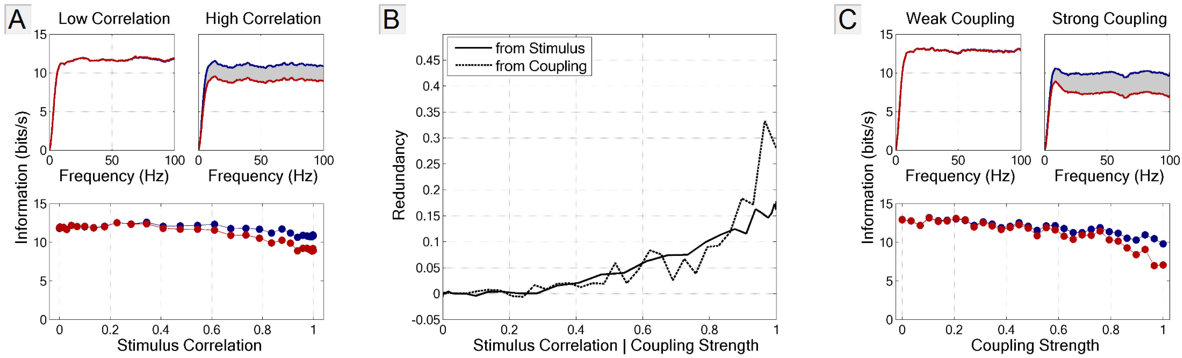
3.4. Multi-Neuron Information and Redundancy

3.4.1. Signal and Intrinsic Correlations

The role of correlations between neurons has been of great interest with respect to population coding. The millisecond [18] and even sub-millisecond [19] precision at which the brain operates in response to external stimuli, in addition to the complexity of features encoded by the brain, necessitates an ensemble of many neurons in the processing of information [20,21]. Historically, the study of multineuronal coding has been limited to methods employing measures of correlation between pairs of neurons. While there is little doubt that the “signal correlations” [22] induced by stimulus alone do not sufficiently account for the levels of correlation found in the brain [23,24] and that the levels of correlation between neurons dynamically adjust in a stimulus-specific manner [25,26,27,28,29], the importance of these correlations in the transmission of information has been debated [30,31,32,33]. More recent measures utilizing information-theoretic approaches [34,35,36] rely on assumptions imposed by a decoder model, in which the amount of information conveyed through pairwise correlations is estimated from the loss or gain of information after correlation assumptions are relaxed (see [36] for further discussion). The lack of tools capable of measuring information carried in neuronal correlations has hindered efforts to measure coding at the population level, despite evidence that encoding procedures require the concerted effort of many neurons [37,38,39,40].
To measure the effects of stimulus correlation on information redundancy, we independently altered the stimulus and the coupling strength between neurons. We first progressively increased the correlation between the stimuli provided to each neuron separately. Adjusting the stimulus correlation was accomplished by generating two uncorrelated stimuli and a third reference stimulus; each neuron was presented with a weighted average between one of the two uncorrelated stimuli and the reference stimulus; the weights thus determined the strength of the correlation with the stimuli driving the two neurons. The resulting stimuli, by virtue of being the sum of two Gaussian distributions with standard deviations, whose sum is less than unity, must be multiplied by an adjustment factor to restore the standard deviation back to a value of one, which in the GLM simulation, is analogous to stimulus contrast. We then increased the coupling strength between neurons, which was determined by a scaling factor applied to the post-spike coupling filter of the GLM simulation (Figure 2A). For this simulation, we used mutually excitatory coupling measures, compensating for the firing rate increases that occur due to the additional excitational input, and measured the effects of these parameters on information rates and redundancy. While the GLM model places no upper limit on the strength of the coupling kernel, we restricted its influence to a reasonable range and report the maximum coupling strength with one and the minimum strength of zero, indicating that the two neurons are uncoupled.
Figure 9A shows the changes in information rates and redundancy as a function of stimulus correlation. The upper panels show typical cumulative information plots when stimuli are nearly completely decorrelated ( r = 0.0019) and when completely correlated ( r = 1 ; the neurons are driven by identical stimuli), with the shaded gray area corresponding to the redundant information. Firing rates did not appreciably change across parameter choices (maximum deviation: 2.8%). As one would predict, increases in redundancy accompany increases in stimulus correlation; neuronal noise prevents complete redundancy. The solid and dotted black lines in Figure 9B show redundancy expressed as a proportion of total information conveyed by the two neurons and demonstrates the effects that increases in stimulus correlation and neuronal coupling strength have on redundancy. Figure 9C shows the reduction in group information that accompanies neuronal coupling.
Figure 9. Signal- and coupling-induced correlations. (A) Effects of signal correlation on redundancy. Responses of two uncoupled neurons to stimuli of increasing correlation are compared. Cumulative information plots of the two extreme cases of low and high stimulus correlation are displayed on top. For low correlation ( r 0 ), group information (red curve) and the sum of information from all the individual cells (blue curve) are nearly identical, due to the lack of correlation in the neural responses; high correlation ( r = 1 ) in the stimulus induces correlation in the neural responses, and the amount of redundant information (shaded gray area) increases. (Bottom) The relationship between stimulus correlation and both group (red) and summed individual total information (blue). (B) Redundancy calculated as a function of stimulus correlation (solid black line) and coupling strength (dotted black line). (C) Effects of neuronal coupling on redundancy. In the upper left panel, neuronal coupling is weak (coupling strength = 0), and the neurons transmit the same (independent) information. In the upper right panel, the coupling is strong (coupling strength = 1), resulting in redundant information (grey area between the group information, shown in red, and total information, shown in blue).
Entropy 15 03507 g009

3.4.2. Application to Large Populations

An important benefit of using the Fourier Method to display neuronal signals in the frequency domain is that the temporal distribution of spiking activity, which is difficult to describe (and becomes prohibitively so as the number of neurons is increased), is transformed into a collection of simple Gaussian distributions, for which the calculation of entropy is straightforward. While the length of the description of spike patterns in the time domain increases as an exponential of the number of neurons ( O 2 N for an N-neuron bit pattern), in the frequency domain, the corresponding calculation is constrained by the speed of diagonalization of the Fourier component covariance matrix; algorithms for this computation, such as the Cholesky decomposition method, have order O N 3 (see, for example, [41]). As a result, the information rates and levels of redundancy for populations of neurons numbering in the hundreds can be calculated on an ordinary desktop computer in a matter of minutes.
An example provided in Figure 10A demonstrates the increase in redundancy as the number of uncoupled neurons responding to the same stimulus progressively increases. Despite the lack of synaptic influence within the network, correlations induced by the stimulus alone are of sufficient magnitude to drastically increase the amount of redundant information (shaded gray area) as the number of neurons increases. The contribution of each successive neuron added to the group decreases, as a fraction of its signal information is inferable from other neurons. It becomes immediately apparent that extrapolation of pairwise redundancy to larger populations can result in egregious misrepresentations of the true signal information rate.
Figure 10B provides information calculation times for groups of up to 500 neurons, calculating up to 100 Hz for 128 trials each. Clearly, the method can easily handle larger neural populations than can be recorded with current technologies. This figure demonstrates the capability of the Fourier information method to scale with large populations of neurons and shows how the influence of both signal and intrinsic correlations affect levels of information and redundancy.
Figure 10. Information in large neural populations. (A) Group size versus sum total and group information using the GLM model. The sum total information, which does not take into account correlations between cells, increases linearly with the number of cells (blue), whereas the group information rate (red) climbs sub-linearly, due to the progressive increase in redundant information (shaded gray area). (B) Processing times on a desktop computer for group sizes of up to 500 neurons. Calculations were performed on an Intel® Core™ i7-3770K running at 3 . 9 GHz with 32 GB RAM.
Entropy 15 03507 g010

4. Summary and Conclusions

We used the GLM framework to simulate single neurons and populations of neurons and explored the influence that various aspects of the discharge and of the interactions between neurons have on our estimate of the amount of information transmitted by the population discharge.
We found that our method is applicable over a wide range of mean firing rates and is robust against both the non-stationarity of the firing rate and errors in the assignment of spikes to neurons in the recorded population. We also described ways to correct for potential inaccuracies in the estimation of information rates from a neural population. Finally, we showed that our method scales to population sizes that exceed the capabilities of current technology and that information in such large groups can be calculated quickly and efficiently.

Acknowledgements

This work was supported by NIH grants EY-1622, NIGMS-1P50GM071558 and NIMH-R21MH093868. We thank Alex Casti for helpful comments on the manuscript.

Conflicts of Interest

The authors declare no conflict of interest.

References

  1. Nicolelis, M.A.L.; Ribeiro, S. Multielectrode recordings: The next steps. Curr. Opin. Neurobiol. 2002, 12, 602–606. [Google Scholar] [CrossRef]
  2. Shannon, C. A mathematical theory of communication. Bell Syst. Tech. J. 1948, 27, 379–423, 623–656, Reprinted with corrections. Available online: http://cm.bell-labs.com/cm/ms/what/shannonday/shannon1948.pdf (accessed on 8 May 2013). [Google Scholar]
  3. Panzeri, S.; Senatore, R.; Montemurro, M.A.; Petersen, R.S. Correcting for the sampling bias problem in spike train information measures. J. Neurophysiol. 2007, 98, 1064–1072. [Google Scholar] [CrossRef]
  4. Quiroga, R.Q.; Panzeri, S. Extracting information from neuronal populations: Information theory and decoding approaches. Nat. Rev. Neurosci. 2009, 10, 173–185. [Google Scholar] [CrossRef] [PubMed]
  5. Ince, R.A.A.; Senatore, R.; Arabzadeh, E.; Montani, F.; Diamond, M.E.; Panzeri, S. Information-theoretic methods for studying population codes. Neural Netw. 2010, 23, 713–727. [Google Scholar] [CrossRef] [PubMed]
  6. Yu, Y.; Crumiller, M.; Knight, B.; Kaplan, E. Estimating the amount of information carried by a neuronal population. Front. Comput. Neurosci. 2010, 4. [Google Scholar] [CrossRef] [PubMed]
  7. Crumiller, M.; Knight, B.; Yu, Y.; Kaplan, E. Estimating the amount of information conveyed by a population of neurons. Front. Neurosci. 2011, 5. [Google Scholar] [CrossRef] [PubMed]
  8. Pillow, J.W.; Paninski, L.; Uzzell, V.J.; Simoncelli, E.P.; Chichilnisky, E.J. Prediction and decoding of retinal ganglion cell responses with a probabilistic spiking model. J. Neurosci. 2005, 25, 11003–11013. [Google Scholar] [CrossRef] [PubMed]
  9. Paninski, L.; Pillow, J.; Lewi, J. Statistical models for neural encoding, decoding, and optimal stimulus design. Prog. Brain Res. 2007, 165, 493–507. [Google Scholar] [PubMed]
  10. Strong, S.P.; Koberle, R.; de Ruyter van Steveninck, R.R.; Bialek, W. Entropy and information in neural spike trains. Phys. Rev. Lett. 1998, 80, 197–200. [Google Scholar] [CrossRef]
  11. Linkser, R. Self-organization in a perceptual network. Computer 1988, 21, 105–117. [Google Scholar]
  12. Pillow, J.W.; Shlens, J.; Paninski, L.; Sher, A.; Litke, A.M.; Chichilnisky, E.J.; Simoncelli, E.P. Spatio-temporal correlations and visual signalling in a complete neuronal population. Nature 2008, 454, 995–999. [Google Scholar] [CrossRef] [PubMed]
  13. Destexhe, A.; Rudolph, M.; Paré, D. The high-conductance state of neocortical neurons in vivo. Nat. Rev. Neurosci. 2003, 4, 739–751. [Google Scholar] [CrossRef] [PubMed]
  14. Destexhe, A.; Paré, D. Impact of network activity on the integrative properties of neocortical pyramidal neurons in vivo. J. Neurophysiol. 1999, 81, 1531–1547. [Google Scholar] [PubMed]
  15. Wilson, C. Up and down states. Scholarpedia J. 2008, 3. [Google Scholar] [CrossRef]
  16. Sherman, S.M. Tonic and burst firing: Dual modes of thalamocortical relay. Trends Neurosci. 2001, 24, 122–126. [Google Scholar] [CrossRef]
  17. Reinagel, P.; Godwin, D.; Sherman, S.M.; Koch, C. Encoding of visual information by LGN bursts. J. Neurophysiol. 1999, 81, 2558–2569. [Google Scholar] [PubMed]
  18. De Charms, R.C.; Merzenich, M.M. Primary cortical representation of sounds by the coordination of action-potential timing. Nature 1996, 381, 610–613. [Google Scholar] [CrossRef] [PubMed]
  19. Carr, C.E. Processing of temporal information in the brain. Annu. Rev. Neurosci. 1993, 16, 223–243. [Google Scholar] [CrossRef] [PubMed]
  20. Braitenberg, V. Cell assemblies in the cerebral cortex. Lecture Notes Biomath. 1978, 21, 171–188. [Google Scholar]
  21. Sakurai, Y. Population coding by cell assemblies–what it really is in the brain. Neurosci. Res. 1996, 26, 1–16. [Google Scholar] [CrossRef]
  22. Gawne, T.J.; Richmond, B.J. How independent are the messages carried by adjacent inferior temporal cortical neurons? J. Neurosci. 1993, 13, 2758–2771. [Google Scholar] [PubMed]
  23. Meister, M.; Lagnado, L.; Baylor, D.A. Concerted signaling by retinal ganglion cells. Science 1995, 270, 1207–1210. [Google Scholar] [CrossRef]
  24. Oram, M.W.; Hatsopoulos, N.G.; Richmond, B.J.; Donoghue, J.P. Excess synchrony in motor cortical neurons provides redundant direction information with that from coarse temporal measures. J. Neurophysiol. 2001, 86, 1700–1716. [Google Scholar] [PubMed]
  25. Eckhorn, R.; Bauer, R.; Jordan, W.; Brosch, M.; Kruse, W.; Munk, M.; Reitboeck, H.J. Coherent oscillations: A mechanism of feature linking in the visual cortex? Biol. Cybern. 1988, 60, 121–130. [Google Scholar] [CrossRef] [PubMed]
  26. Gray, C.M.; König, P.; Engel, A.K.; Singer, W. Oscillatory responses in cat visual cortex exhibit inter-columnar synchronization which reflects global stimulus properties. Nature 1989, 338, 334–337. [Google Scholar] [CrossRef] [PubMed]
  27. Vaadia, E.; Haalman, I.; Abeles, M.; Bergman, H.; Prut, Y.; Slovin, H.; Aertsen, A. Dynamics of neuronal interactions in monkey cortex in relation to behavioural events. Nature 1995, 373, 515–518. [Google Scholar] [CrossRef] [PubMed]
  28. Steinmetz, P.N.; Roy, A.; Fitzgerald, P.J.; Hsiao, S.S.; Johnson, K.O.; Niebur, E. Attention modulates synchronized neuronal firing in primate somatosensory cortex. Nature 2000, 404, 187–190. [Google Scholar] [CrossRef] [PubMed]
  29. Wang, Y.; Iliescu, B.F.; Ma, J.; Josić, K.; Dragoi, V. Adaptive changes in neuronal synchronization in macaque V4. J. Neurosci. 2011, 31, 13204–13213. [Google Scholar] [CrossRef] [PubMed]
  30. Nirenberg, S.; Carcieri, S.M.; Jacobs, A.L.; Latham, P.E. Retinal ganglion cells act largely as independent encoders. Nature 2001, 411, 698–701. [Google Scholar] [CrossRef] [PubMed]
  31. Levine, M.W.; Castaldo, K.; Kasapoglu, M.B. Firing coincidences between neighboring retinal ganglion cells: Inside information or epiphenomenon? Biosystems 2002, 67, 139–146. [Google Scholar] [CrossRef]
  32. Averbeck, B.B.; Lee, D. Neural noise and movement-related codes in the macaque supplementary motor area. J. Neurosci. 2003, 23, 7630–7641. [Google Scholar] [PubMed]
  33. Golledge, H.D.R.; Panzeri, S.; Zheng, F.; Pola, G.; Scannell, J.W.; Giannikopoulos, D.V.; Mason, R.J.; Tovée, M.J.; Young, M.P. Correlations, feature-binding and population coding in primary visual cortex. Neuroreport 2003, 14, 1045–1050. [Google Scholar] [PubMed]
  34. Brenner, N.; Strong, S.P.; Koberle, R.; Bialek, W.; de Ruyter van Steveninck, R.R. Synergy in a neural code. Neural Comput. 2000, 12, 1531–1552. [Google Scholar] [CrossRef] [PubMed]
  35. Abbott, L.F.; Dayan, P. The effect of correlated variability on the accuracy of a population code. Neural Comput. 1999, 11, 91–101. [Google Scholar] [CrossRef] [PubMed]
  36. Latham, P.E.; Nirenberg, S. Synergy, redundancy, and independence in population codes, revisited. J. Neurosci. 2005, 25, 5195–5206. [Google Scholar] [CrossRef] [PubMed]
  37. Abeles, M.; Bergman, H.; Margalit, E.; Vaadia, E. Spatiotemporal firing patterns in the frontal cortex of behaving monkeys. J. Neurophysiol. 1993, 70, 1629–1638. [Google Scholar] [PubMed]
  38. Maldonado, P.E.; Gerstein, G.L. Neuronal assembly dynamics in the rat auditory cortex during reorganization induced by intracortical microstimulation. Exp. Brain Res. 1996, 112, 431–441. [Google Scholar] [CrossRef] [PubMed]
  39. Nicolelis, M.A.; Lin, R.C.; Chapin, J.K. Neonatal whisker removal reduces the discrimination of tactile stimuli by thalamic ensembles in adult rats. J. Neurophysiol. 1997, 78, 1691–1706. [Google Scholar] [PubMed]
  40. Ikegaya, Y.; Aaron, A.; Cossart, R.; Aronov, D.; Lampl, I.; Ferster, D.; Yuste, R. Synfire chains and cortical songs: Temporal modules of cortical activity. Science 2004, 304, 559–564. [Google Scholar] [CrossRef] [PubMed]
  41. Watkins, D.S. Fundamental of Matrix Computations, 1st ed.; Wiley: New York, NY, USA, 1991; p. 84. [Google Scholar]

