1. Introduction
The motivation behind specialization on DNA compression comes from the fact that general purpose compression algorithms are far from optimum and are not aware of the particularities of DNA sequences. The huge growth in DNA databases urges for better compression algorithms, and the increasing knowledge on DNA structure allows one to design compression algorithms that take advantage of its particularities and redundancies, as, for example, the so-called complemented inverted repeats.
The first encoder specialized in DNA compression was proposed in 1993 [
1].
Biocompress, as the authors named it, uses a substitution approach similar to the well-known Lempel-Ziv [
2] coding scheme, but featured a mechanism to consider not only repetitions, but also complementary palindromes, as well. A second version,
Biocompress-2, includes an order-2 finite-context model (FCM) as a fall-back scheme [
3].
Besides other substitutional encoders, such as [
4], an innovative model was proposed in [
5], where several predictors based on inexact matches are combined and are used to estimate the entropy of DNA. Three years later, an algorithm employing context-tree weighting and substitutional compression was published [
6], which used context-tree weighting whenever the substitutional approach yielded worse results. Furthermore, using a substitutional approach,
GenCompress-1 and
GenCompress-2 [
7] generalized this concept, relying on operations, such as replacements, insertions and deletions, in order to transform a given past sub-string into the sub-string to be encoded.
The use of finite-context models regained attention in [
8], again, as a fall-back algorithm, where the main algorithm, a normalized maximum likelihood substitutional approach, is replaced by an order-2 FCM whenever better and, as a last-resort, by a transparent mode.
Moreover, in [
9], order-2 and order-3 FCMs were also used as fall-back mechanisms, in a substitutional-like compressor aimed at speed, giving more attention to the substitution of large sequences, rather than to small ones.
This approach was mainly improved by [
10,
11]. The state-of-the-art compressor expert model (XM) [
12] uses various experts consisting of order-1 and order-2 FCMs and a copy-expert that creates a symbolic dependence between the next symbol and a previously occurring one. The data-fusion of this expert mixture is made using Bayesian averaging and is followed by an arithmetic encoder. As such, up to this point, much of the work was based on the substitutional method, and if low performance is obtained, a low-order FCM is used.
Finally, FCM gained protagonism in [
13,
14,
15,
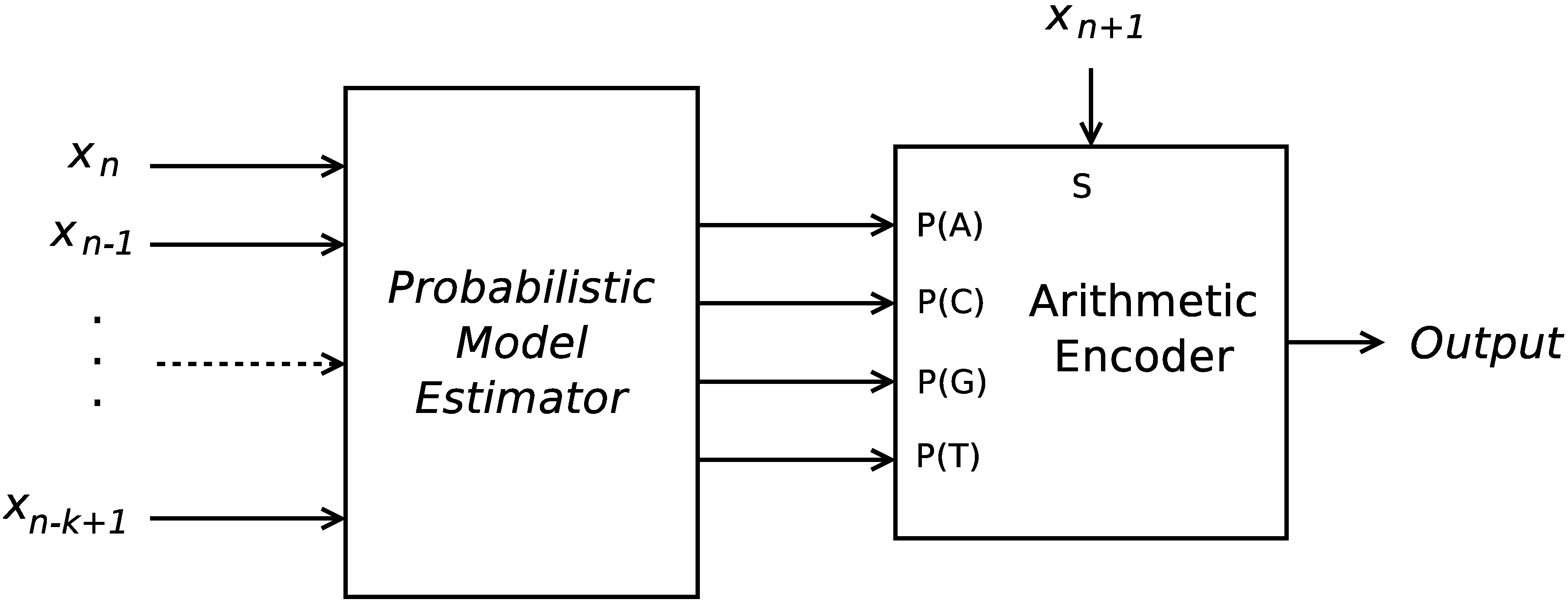
16], implemented up to order-16. As in the previous cases, the FCMs were followed by an arithmetic encoder, and several different-order FCMs compete. However, now, only this type of predictor was employed. This architecture lays on what is generally described as a probabilistic model estimator and an arithmetic encoder, as is depicted in
Figure 1. The results show that, despite the simplicity of the algorithm, some sub-sequences can be accurately modeled by such models, which suggests that a short-term memory system such as this can make reasonable predictions in comparison to long-term memory systems as those employing the substitutional paradigm. Moreover, the encoder is very fast, in addition to achieving an encoding ratio similar to that obtained by the state-of-the-art Expert Model [
11].
Figure 1.
Structure of an encoder architecture, which employs a probabilistic model estimator and an arithmetic encoder for the symbols {A, C, G, T}.
Figure 1.
Structure of an encoder architecture, which employs a probabilistic model estimator and an arithmetic encoder for the symbols {A, C, G, T}.
The speed and the inherent simplicity of such an algorithm are great features, which makes it suitable for hardware implementations, such as field-programmable gate arrays (FPGAs), which would translate into high-performance compressors for high throughput sequencers. However, a major challenge of such an implementation is that, when the order of such FCMs is increased, the memory requirements increase exponentially, as order-N requires memory entries (the actual memory required is dependent on the size of each entry). This problem can be minimized by using hash-tables, thus allocating memory only when a new conditioning context is encountered. However, this not only increases the complexity of such a system if it is intended to be implemented in FPGA, but also fails to address the memory requirement problem if very large sequences are to be encoded, as a large variety of conditioning contexts exist.
To tackle this memory/complexity problem, this paper proposes a novel architecture that has lower memory requirements and uses a well-known technology. To achieve that, the high-order memory intensive FCMs are replaced by artificial neural networks (ANNs), which have the particularity of being a compact way to interpolate data and for which a FPGA implementation is feasible. Such ANNs are used simultaneously with low-order FCMs, in a competitive fashion, using a forward-adaptive method, like the one presented in [
14], which chooses which of the models is best suited to encode the next block and sends an identifier of the selected model as side information.
This work was particularly focused on bacterial DNA, due to their high entropy and few repeating regions, being thus harder to effectively encode, strengthening the need for specialized compressors.
To implement a DNA compressor using ANNs, several aspects must be addressed. After this introductory section, Section II presents how the data should be formatted at the input of the ANN and what targets should be used as training data. Section III formalizes the problem and specifies how should the training be performed in an effective way. Then, Section IV presents experimental results against other existing DNA compression methods using bacterial DNA sequences from the National Center for Biotechnology Information (NCBI) database, and finally, Section V draws some conclusions and points out some future work.
2. Data Representation
DNA sequences are coded by four bases, commonly represented within the alphabet,
. Due to the symbolic (hence, unordered) nature of these bases, care should be taken to keep the system independent of any relabelling between symbols when representing and manipulating the data in a computer environment. To cope with such a requirement, the data must be kept symbolic across the ANN rather than assigning numeric values to each symbol, which is commonly referred to as a classification problem [
17,
18]. In this scenario, each base is coded as an
N-tuple, where each element refers to a symbol, and all elements are zero, except the one corresponding to the coding symbol, which is set to one. Usually, in practical implementations, the values,
and
, are used instead, since the sigmoidal activation functions have limits on these two values, thus requiring high weight values on the input branches.
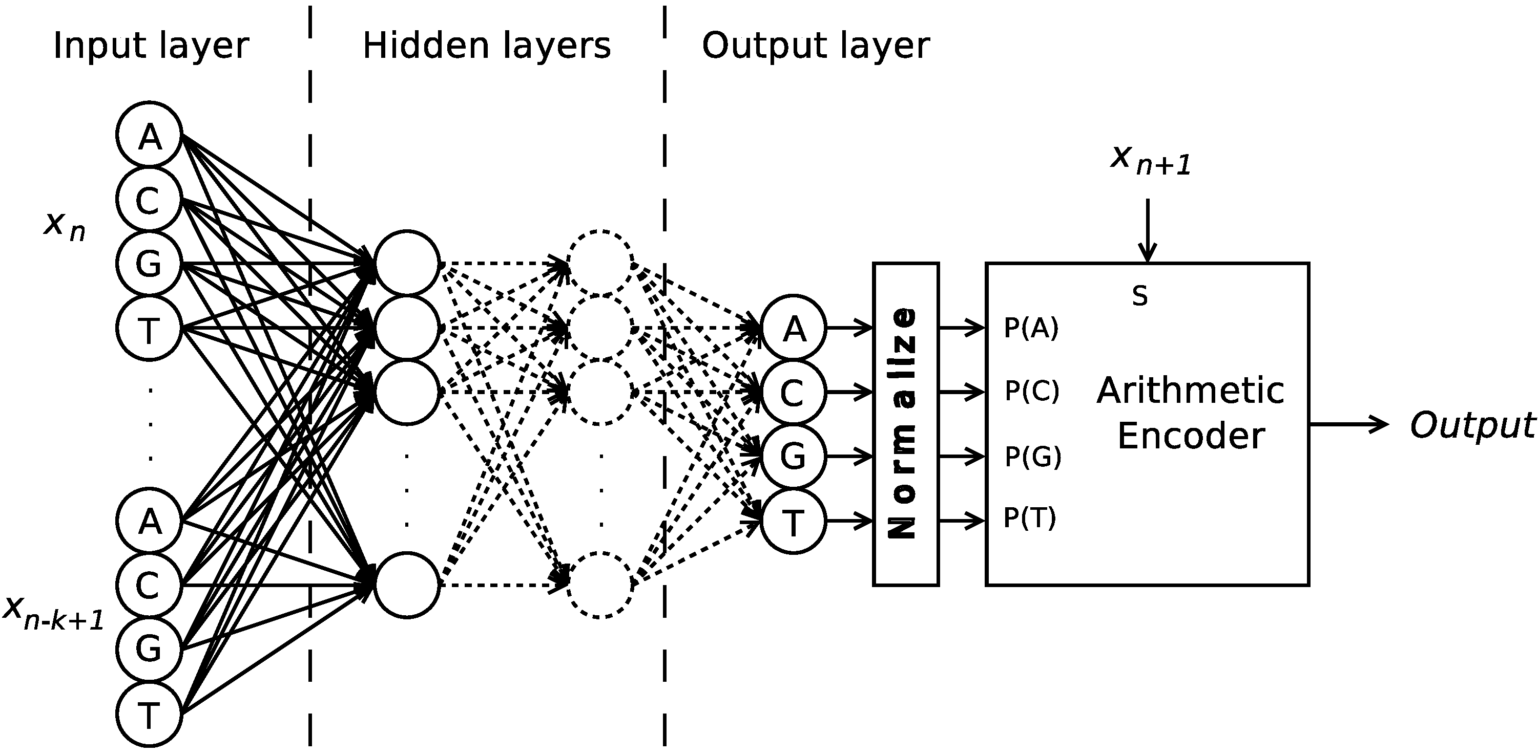
Regarding the output, regular ANNs relate the input with the output deterministically. As such, since finite-context modelling is a non-deterministic problem—for the same preceding sequence, the next symbol, , has a probabilistic model associated with it, —such deterministic output is likely to be wrong. Moreover, when an ANN is trained, at each iteration, the weights of all connecting edges, usually denoted by a single weight vector, , or a set of matrices, are optimized to minimize the result of a given cost function for a set—training set—of input/output (or target) pairs. However, if the next symbol, , is not related to the input, , deterministically, the neural network is likely to fail converging during training and on making useful estimations.
To overcome this, the target outputs used for training should not be the symbols
per se, but their probabilistic model instead. This method not only provides a deterministic output (for the same conditioning context, the same probabilistic model should be used), but also simplifies the implementation, as the output of the ANN can be used, after normalization, directly to feed the arithmetic encoder, as depicted in
Figure 2.
Figure 2.
Structure of the Time-Series Artificial Neural Network proposed. The bias units within the hidden layers are omitted for readability.
Figure 2.
Structure of the Time-Series Artificial Neural Network proposed. The bias units within the hidden layers are omitted for readability.
This configuration was used along with FCMs. To do that, an approach similar to [
14] was taken: the sequence data is split in blocks, and for each block, all the probabilistic models are evaluated. The best one, the one which yields a lower entropy, is selected to encode the block, and an identifier of the model is coded as side information. A simple probabilistic model of the side information is maintained to compress it, too, using the arithmetic encoder. This competitive fashion allows the use of several models, and the final result is the minimum entropy of all models at each block, plus the side information.
4. Experimental Results
To compare the proposed models in terms of encoding efficiency, three reference encoders were used. One third-party encoder, called XM [
12] was composed of a set of 500 expert models, hereafter referred to as XM-500. Another composed of a mixture of eight finite-context models with order-2, -4, -6, -8, -10, -12, -14 and -16, hereafter referred to as FCM-M16. The last one, hereafter referred to as FCM-M10, was composed of order-2, -4, -6, -8 and -10. For model order-2, -4, -6 and -8,
, for model order-10, -12 and -14,
, and, finally, for order-16,
. All these implementations were those originally used by their authors. Therefore, the XM-500 implementation was written in Java, and the FCM compressors were written in C.
Three encoder configurations employing the proposed model were chosen. Two of them were based on FCMs with order-2, -4, -6, -8 and -10, using for all contexts, except order-10, which used . Additionally, competing with these finite-context models, one neural network was added to each encoder. The encoder, hereafter referred to as NN1 (neural-network 1), used an ANN with a memory depth of 40 and 15 hidden nodes in its single hidden layer. The encoder, hereafter referred to as NN2, used an ANN with a memory depth of 16 and 15 hidden nodes. The third encoder, hereafter referred to as NN3, was composed of FCMs similar to FCM-M16, but with an additional artificial neural network similar to the one used in NN2. This last configuration was aimed at improving just the coding efficiency, as it brings no advantages regarding run-time memory requirements. Due to the nature of these compressors, they were all implemented over the original FCM source code, in the C language, and compiled using GCC (GNU C Compiler). Additionally, 7-Zip version 9.04 and PAQ12a were used for comparison against the special-purpose encoders.
Since this compressor is aimed at DNA sequences, it was evaluated using a large database of bacterial DNA sequences, namely, the one from the National Center for Biotechnology Information [
19], which has
complete sequences (without uncertainty) ranging from
to
bases and totalling
bases.
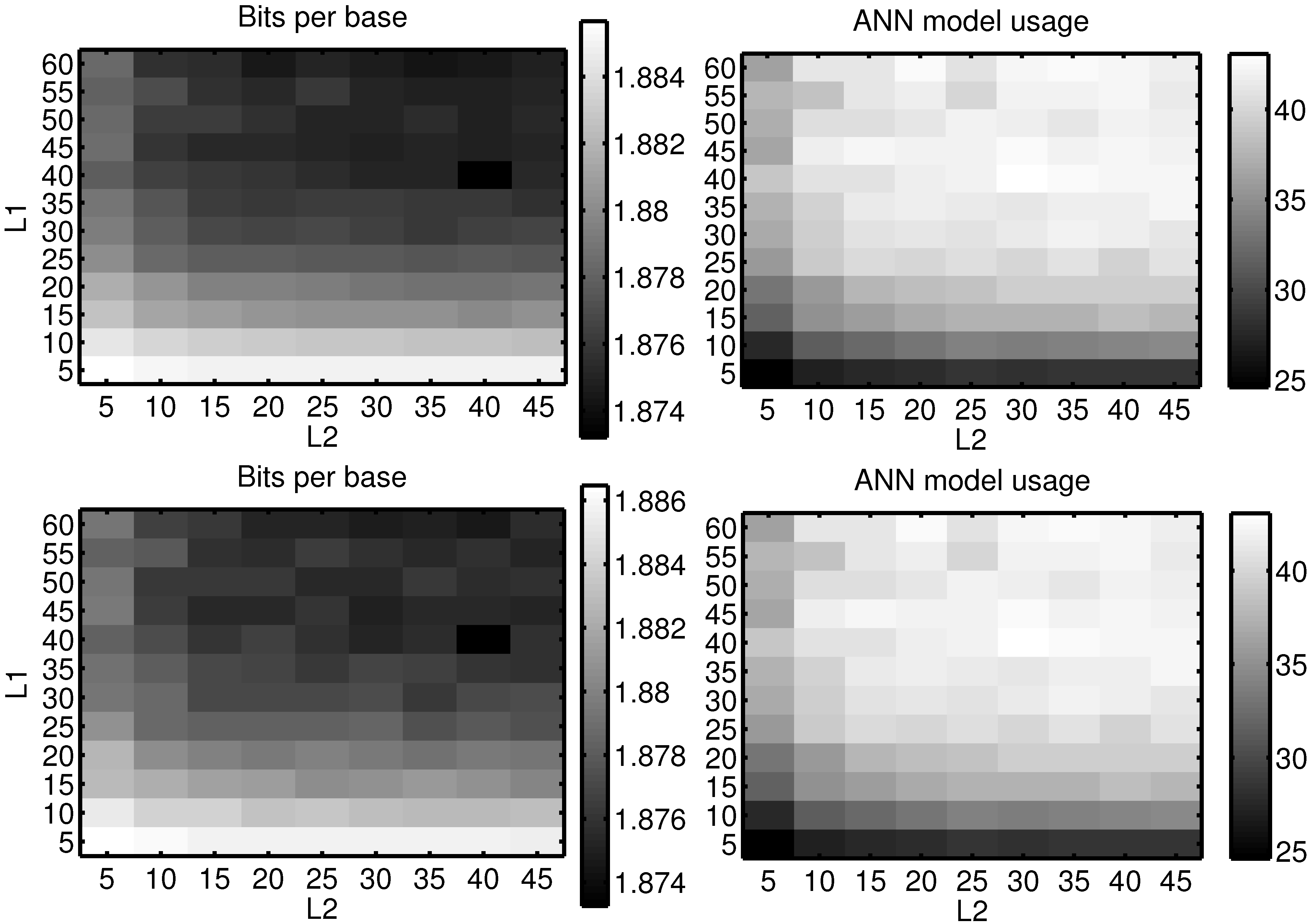
Unfortunately, there is no proven method to choose the number of layers and their size for an artificial neural network. As such, these values were selected by sweeping the memory depth and hidden node count from two to 40, and five to 30, respectively, and choosing the best compromise, taking into account not only the encoding ratio, but also the encoding time, as for larger networks the encoding time becomes impractical. The learning rate,
η, used was five, which was the value that yielded the best results for a subset of NCBI bacteria DNA database and which have proven to give satisfying results over the rest of the set. Nevertheless, these results are not highly dependent on small variations of the node count. To illustrate that,
Figure 3 shows the overall bits-per-base and the usage-ratio of the ANN model, when sweeping the memory depth from five to 60 and the hidden node count from five to 45 on the NN1 encoder. This was carried out on two uncorrelated random subsets of the complete data-set used in the rest of the work. It can be seen that there are no discontinuities in the plot and that the bits-per-base and usage surfaces are smooth.
Three parameters were measured during simulations: the overall bits-per-base (bpb), the overall encoding time in microseconds per base (
μspb) and the run-time memory required. These results are summarized in
Table 1, which represents the performance over all
sequences.
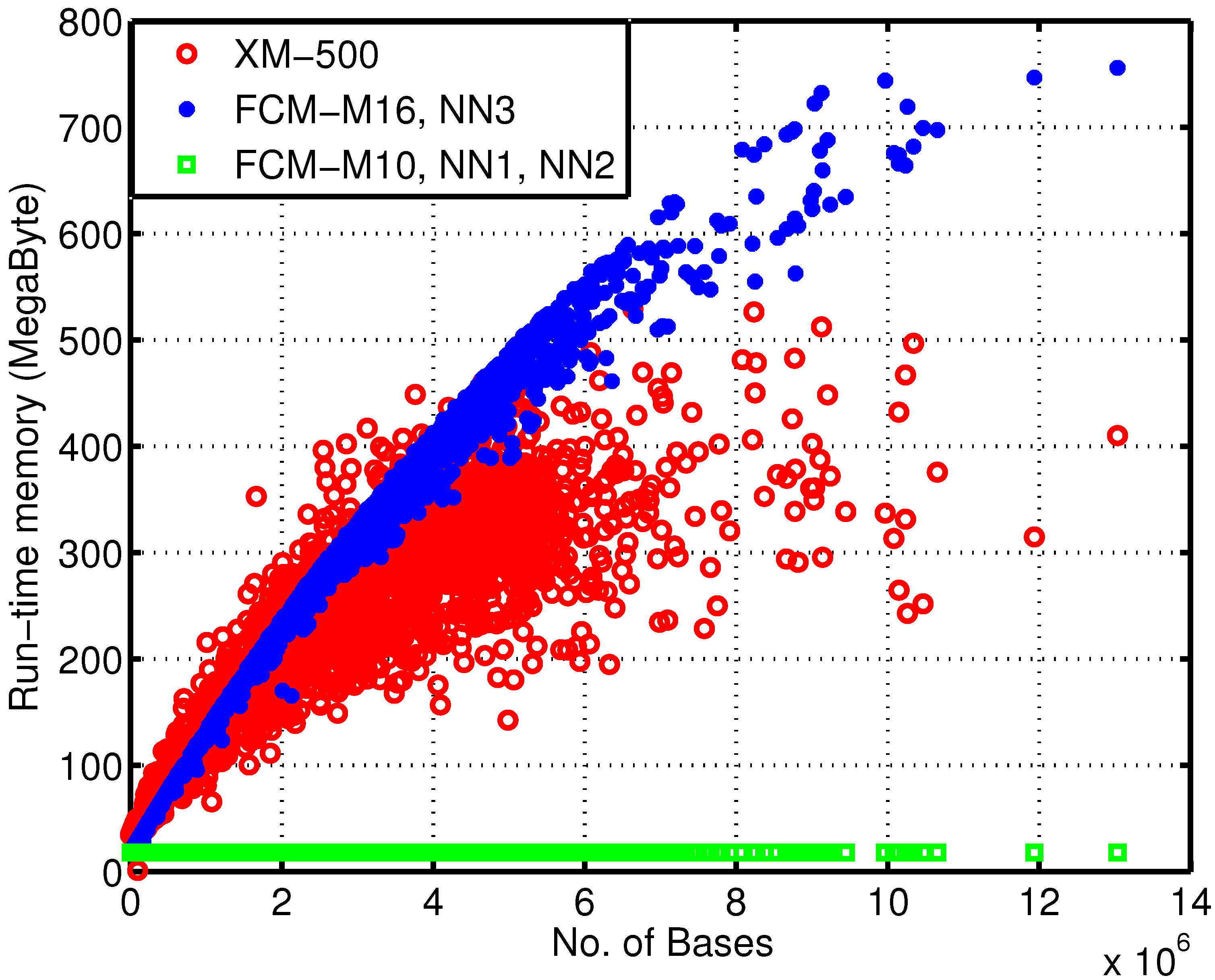
Figure 4 depicts the memory usage dependency over the number of bases for each sequence. In regards to memory, due to the 64-bit nature of the machine where these simulations were carried out, each finite-context memory entry uses four bytes and each ANN weight uses eight bytes. Regarding the execution time, all implementations were run in the same machine, an Intel Core 2 Duo P8600 at a constant clock frequency of 2.4 GHz and with 4 GiB of RAM.
In
Figure 4, the discrepancy between the reference and the proposed encoders is clear. Moreover, note that the 17 MB used by encoders FCM-M10, NN1 and NN2 are mainly due to the order-10 FCM, which requires
memory entries, since the largest ANN is estimated to occupy the negligible amount of 20 k floating-point memory entries.
Figure 3.
Bits-per-base and artificial neural network (ANN) model usage, for the NN1 encoder, by sweeping the memory depth (L1) and the hidden node count (L2). Two different subsets were used.
Figure 3.
Bits-per-base and artificial neural network (ANN) model usage, for the NN1 encoder, by sweeping the memory depth (L1) and the hidden node count (L2). Two different subsets were used.
Table 1.
Simulation results of the seven encoders used, over all sequences, depicting bits-per-base, μs per base and the average run-time memory required. bpb, bits-per-base; μspb, overall encoding time in microseconds per base; FCM, finite-context model; NN, neural-network; XM, expert model.
Table 1.
Simulation results of the seven encoders used, over all sequences, depicting bits-per-base, μs per base and the average run-time memory required. bpb, bits-per-base; μspb, overall encoding time in microseconds per base; FCM, finite-context model; NN, neural-network; XM, expert model.
| Encoder Name | bpb | μspb | Average memory | Maximum memory |
|---|
| FCM-M10 | 1.8659 | 1.3891 | 17 MB | 17 MB |
| NN1 | 1.8491 | 13.6570 | 17 MB | 17 MB |
| NN2 | 1.8551 | 7.0582 | 17 MB | 17 MB |
| FCM-M16 | 1.8498 | 4.3899 | 195 MB | 738 MB |
| NN3 | 1.8395 | 10.0271 | 195 MB | 738 MB |
| XM-500 | 1.8578 | 10.2196 | 31 MB | 521 MB |
| 7-Zip | 2.1402 | 1.0711 | - | - |
| PAQ12a | 2.0205 | 1.3887 | - | - |
Figure 4.
Run-time memory usage of the encoders over the number of bases of each sequence. This dependency arises from the fact that, for models of an order higher than 10, hash-tables are used to minimize the memory allocated.
Figure 4.
Run-time memory usage of the encoders over the number of bases of each sequence. This dependency arises from the fact that, for models of an order higher than 10, hash-tables are used to minimize the memory allocated.
Regarding these results, all three encoders, NN1, NN2 and NN3, have particular properties. In regards to computing time, NN1 is the slowest, due to the size of the neural network used. Moreover, its advantage over NN2 is not significant. NN3, on the other hand, has the best encoding ratio, with the same memory requirements as FCM-M16 and slightly less encoding time than XM-500. Finally, NN2 represents a good compromise between coding efficiency, time and memory used, as its coding efficiency is almost the same as XM-500, but slightly worse than FCM-M16. Additionally, its computation time is the third best among all encoders used. Moreover, it uses slightly less than 17 MB, against the average 195 MB (maximum 738 MB) of FCM-M16. FCM-M10, although the fastest, yielded the worst encoding efficiency, which reinforces the fact that an additional neural network indeed increases the coding performance.
Additionally, the competition among the various models was also measured, as it indicates the importance of each model in the encoding results presented previously. These are presented in
Table 2,
Table 3 and
Table 4.
Table 5 is used to compare the effect of the additional ANN in NN1 and NN2 over the FCM.
Inspecting
Table 2, for example, the first line indicates that the order-2 FCM was used in
of the 100-bases blocks, and from those, the mean bpb is
. As such, up to order-6, all FCMs have an average bpb higher than ANN 40:15, which was used
of the time, with a mean average of
bpb. Note, although, that the low-order FCMs were used whenever all the other models yielded worse results for the same block.
In
Table 4, the model usage of ANN 16:15 decreases slightly, but keeps close to 40%. Note that although the order-16 FCM exhibits an impressive 1.18 bpb, it was only used 4% of the time, which means that it was able to accurately model small regions of the sequences. However, in all the other 96% of the blocks, the other models were better.
Table 2.
Average model usage and compression ratio for NN1 over all sequences.
Table 2.
Average model usage and compression ratio for NN1 over all sequences.
| Model Name | Usage (%) | bpb |
|---|
| order-2 | 8.52 | 1.9211 |
| order-4 | 13.32 | 1.8839 |
| order-6 | 19.34 | 1.8529 |
| order-8 | 10.36 | 1.8315 |
| order-10 | 3.27 | 1.1996 |
| ANN 40:15 | 45.19 | 1.8388 |
Table 3.
Average model usage and compression ratio for NN2 over all sequences.
Table 3.
Average model usage and compression ratio for NN2 over all sequences.
| Model Name | Usage (%) | bpb |
|---|
| order-2 | 8.67 | 1.9228 |
| order-4 | 13.32 | 1.8843 |
| order-6 | 21.36 | 1.8516 |
| order-8 | 12.30 | 1.8300 |
| order-10 | 3.49 | 1.2103 |
| ANN 16:15 | 40.85 | 1.8499 |
Table 4.
Average model usage and compression ratio for NN3 over all sequences.
Table 4.
Average model usage and compression ratio for NN3 over all sequences.
| Model Name | Usage (%) | bpb |
|---|
| order-2 | 7.63 | 1.9107 |
| order-4 | 12.77 | 1.8797 |
| order-6 | 20.84 | 1.8489 |
| order-8 | 11.82 | 1.8286 |
| order-10 | 0.93 | 1.6918 |
| order-12 | 0.63 | 1.6068 |
| order-14 | 2.19 | 1.7897 |
| order-16 | 4.02 | 1.1839 |
| ANN 16:15 | 39.18 | 1.8443 |
Table 5.
Average model usage and compression ratio for FCM-M10 over all sequences.
Table 5.
Average model usage and compression ratio for FCM-M10 over all sequences.
| Model Name | Usage (%) | bpb |
|---|
| order-2 | 17.24 | 1.9303 |
| order-4 | 23.74 | 1.8887 |
| order-6 | 36.60 | 1.8547 |
| order-8 | 18.49 | 1.8354 |
| order-10 | 3.93 | 1.2393 |
In conclusion, from these tables, we see that although ANNs do not have an overall low bpb, its usage percentage indicates that they are better than all the FCMs of the time and, as such, contribute to the reduction of the average bpb, as can be confirmed by the model usage and overall bpb of the plain FCM-M10 encoder.
5. Conclusions
In this work, it was verified that artificial neural networks are an effective way to compress data using a fraction of the run-time memory of the other encoders and, as such, to compact probabilistic models of data. Moreover, this architecture opens the way for the use of more complex machine learning techniques for probability-model estimation, which could be used in other areas of information theory. Despite the fact that FCMs have the ability to detect very low entropy regions where ANNs do not, two conclusions may be drawn from this. On the one hand, ANNs should be used along with FCMs, but, on the other hand, the finite-context order does not need to be too large. It is important to note that although large ANNs have encoding time as major a disadvantage, their simplicity and low memory requirement make them suitable for high-performance hardware, such as FPGAs.
Regarding the dimensioning of the ANN, unfortunately, there is no proven method to select an optimal ANN architecture. As such, other configurations could prove to be better. More work could be developed in this area. Moreover, if advances are made in this application of ANNs and a low-entropy is obtained, it is easier to draw biological conclusions from the strength of each neural network connection at the input layer, as it indicates the importance of each previous base to predict the next one, which is commonly referred to as dimensionality reduction.
Future work may consist in the evaluation of the performance of the encoder using fixed-point arithmetic within the ANN, so that the encoder could be effectively implemented in an FPGA. Moreover, since artificial neural networks were used only as a proof-of-concept, other machine learning techniques, such as support vector machines or deep-learning, can be used in this encoder architecture. Therefore, further investigation of different methods would be very interesting.


