Synchronization of a Class of Fractional-Order Chaotic Neural Networks

Abstract

The synchronization problem is studied in this paper for a class of fractional-order chaotic neural networks. By using the Mittag-Leffler function, M-matrix and linear feedback control, a sufficient condition is developed ensuring the synchronization of such neural models with the Caputo fractional derivatives. The synchronization condition is easy to verify, implement and only relies on system structure. Furthermore, the theoretical results are applied to a typical fractional-order chaotic Hopfield neural network, and numerical simulation demonstrates the effectiveness and feasibility of the proposed method.

1. Introduction

Fractional calculus has been a 300-year-old topic. Although it has a long mathematical history, the applications of fractional calculus to physics and engineering are only a recent focus of interest. Recent monographs and symposia proceedings have highlighted the application of fractional calculus in physics, continuum mechanics, signal processing, bioengineering, diffusion wave and electromagnetics [1,2,3,4]. The major advantage of the fractional-order derivatives is that they provide an excellent instrument for the description of memory and hereditary properties of various materials and processes. As such, some researchers introduced fractional calculus to neural networks to form fractional-order neural networks, which can better describe the dynamical behavior of the neurons, such as “memory". It was pointed out that fractional derivatives provide neurons with a fundamental and general computation ability that can contribute to efficient information processing, stimulus anticipation and frequency-independent phase shifts of oscillatory neuronal firing [5]. It is suggested that the oculomotor integrator, which converts eye velocity into eye position commands, may be of a fractional order [6]. It was demonstrated that neural network approximation taken at the fractional level resulted in higher rates of approximation [7]. Furthermore, note that fractional-order recurrent neural networks might be expected to play an important role in parameter estimation. Therefore, the incorporation of memory terms (a fractional derivative or integral operator) into neural network models is an important improvement [8], and it will be of important significance to study fractional-order neural networks.

Chaos has been a focus of intensive discussion in numerous fields during the last four decades. Moreover, it has been verified that some neural networks can exhibit chaotic dynamics. For example, experimental and theoretical studies have revealed that a mammalian brain not only can display in its dynamical behavior strange attractors and other transient characteristics for its associative memories, but also can modulate oscillatory neuronal synchronization by selective visual attention optimization problems [9,10]. In recent years, the study on synchronization of chaotic neural networks has attracted considerable attention, due to the potential applications in many fields, including secure communication, parallel image processing, biological systems, information science, etc. As we know, there are many synchronization results about integer-order neural networks; see [11,12,13] and references therein. On the other hand, since bifurcations and chaos of fractional-order neural networks were investigated firstly in [14,15], some important and interesting results about fractional-order neural networks have been obtained. For instance, in [16], a fractional-order Hopfield neural model was proposed, and its stability was investigated by an energy-like function. Chaos and hyperchaos in fractional-order cellular neural networks was discussed in [17]. Yu et al. [18] investigated α-stability and α-synchronization for fractional-order neural networks. Several recent results concerning chaotic synchronization in fractional-order neural networks have been reported in [19,20,21,22].

Due to the complexity of fractional-order systems, to the best of our knowledge, there are few theoretical results on the synchronization of fractional-order neural networks; most of the existing results are only numerical simulation [19,20,21,22]. Although there have been many synchronization results about integer-order neural networks in the past few decades, these results and methods could not be extended and applied easily to the fractional-order case. Therefore, to establish some theoretical sufficient criteria for the synchronization of fractional-order neural networks is very necessary and challenging. Motivated by the above discussions, by using the Mittag-Leffler function, some properties of fractional calculus and linear feedback control, a simple and efficient criterion in terms of the M-matrix for synchronization of such neural network is derived. Numerical simulations also demonstrate the effectiveness and feasibility of the proposed technique.

The rest of the paper is organized as follows. Some necessary definitions and lemmas are given, and the fractional-order network model is introduced in Section 2. A sufficient criterion ensuring the synchronization of such neural networks is presented in Section 3. An example and simulation are obtained in Section 4. Finally, the paper is concluded in Section 5.

2. Preliminaries and System Description

In this section, some definitions of fractional calculation are recalled and some useful lemmas are introduced.

Definition 1

[1]. The fractional integral (Riemann-Liouville integral), $D_{t_0,t}^{-\alpha }$, with fractional order, $\alpha \in R^{+}$, of function $x(t)$ is defined as:

$$\begin{array}{c}\hfill D_{t_0,t}^{-\alpha }x(t)=\frac{1}{\Gamma (\alpha )}{\int }_{t_0}^t{(t-\tau )}^{\alpha -1}x(\tau )d\tau \end{array}$$

(1)

where $\Gamma (·)$ is the gamma function, $\Gamma (\tau )={\int }_0^{\infty }{t}^{\tau -1}{e}^{-t}dt$.

Definition 2

[1]. The Riemann-Liouville derivative of fractional order α of function $x(t)$ is given as:

$$\begin{array}{ccc}\hfill {}_{RL}{D}_{t_0,t}^{\alpha }x(t)& =& \frac{d^n}{d{t}^n}{D}_{t_0,t}^{-(n-\alpha )}x(t)=\frac{d^n}{d{t}^n}\frac{1}{\Gamma (n-\alpha )}{\int }_{t_0}^t{(t-\tau )}^{n-\alpha -1}x(\tau )d\tau \hfill \end{array}$$

(2)

where $n-1<\alpha <n\in Z^{+}$.

Definition 3

[1]. The Caputo derivative of fractional order α of function $x(t)$ is defined as follows:

$$\begin{array}{ccc}\hfill {}_C{D}_{t_0,t}^{\alpha }x(t)& =& D_{t_0,t}^{-(n-\alpha )}\frac{d^n}{d{t}^n}x(t)=\frac{1}{\Gamma (n-\alpha )}{\int }_{t_0}^t{(t-\tau )}^{n-\alpha -1}{x}^{(n)}(\tau )d\tau \hfill \end{array}$$

(3)

where $n-1<\alpha <n\in Z^{+}$.

Note from Equations (2) and (3) that the fractional derivative is related to all the history information of a function, while the integer one is only related to its nearby points. That is, the next state of a system not only depends upon its current state, but also upon its historical states starting from the initial time. As a result, a model described by fractional-order derivatives possesses memory and inheritance and will be more precise to describe the states of neurons. In the following, the notation, $D^{\alpha }$, is chosen as the Caputo derivative, $D_{0,t}^{\alpha }$. For $x\in R^n$, the norm is defined by $\parallel x\parallel ={\sum }_{i=1}^n|x_i|$.

Definition 4

[1]. The Mittag-Leffler function with two parameters appearing is defined as:

$$\begin{array}{c}\hfill E_{\alpha ,\beta }(z)={\displaystyle \sum _{k=0}^{\infty }}\frac{z^k}{\Gamma (k\alpha +\beta )}\end{array}$$

(4)

where $\alpha >0,\beta >0$, and $z\in C$. When $\beta =1$, one has $E_{\alpha }(z)=E_{\alpha ,1}(z)$, further, $E_{1,1}(z)=e^z$.

Lemma 1.

Let $V(t)$ be a continuous function on $[0,+\infty )$ and satisfy:

$$\begin{array}{c}\hfill D^{\alpha }V(t)\le -\lambda V(t)\end{array}$$

(5)

Then:

$$\begin{array}{c}\hfill V(t)\le V(t_0)E_{\alpha }(-\lambda {(t-t_0)}^{\alpha })\end{array}$$

(6)

where $\alpha \in (0,1)$ and λ are positive constant.

Proof. 

It follows from Equation (5) that there exists a nonnegative function, $M(t)$, such that:

$$\begin{array}{c}\hfill D^{\alpha }V(t)+\lambda V(t)+M(t)=0\end{array}$$

(7)

Taking the Laplace transform on Equation (7), then one has:

$$\begin{array}{c}\hfill s^{\alpha }V(s)-s^{\alpha -1}V(t_0)+\lambda V(s)+M(s)=0\end{array}$$

(8)

where $V(s)=L\{V(t)\},M(s)=L\{M(t)\}$. It then follows that:

$$\begin{array}{c}\hfill V(s)=\frac{s^{\alpha -1}V(t_0)-M(s)}{s^{\alpha }+\lambda }\end{array}$$

(9)

Taking the inverse Laplace transform in Equation (9), one obtains:

$$\begin{array}{c}\hfill V(t)=V(t_0)E_{\alpha }(-\lambda {(t-t_0)}^{\alpha })-M(t)*[{(t-t_0)}^{\alpha -1}{E}_{\alpha ,\alpha }(-\lambda {(t-t_0)}^{\alpha })]\end{array}$$

(10)

Note that both ${(t-t_0)}^{\alpha }$ and $E_{\alpha ,\alpha }(-\lambda {(t-t_0)}^{\alpha })$ are nonnegative functions; it follows that:

$$\begin{array}{c}\hfill V(t)\le V(t_0)E_{\alpha }(-\lambda {(t-t_0)}^{\alpha })\end{array}$$

(11)

Lemma 2

[1]. If $\alpha <2$, β is an arbitrary real number, μ is such that $\pi \alpha /2<\mu <min\{\pi ,\pi \alpha \}$ and C is a real constant, then:

$$\begin{array}{c}\hfill |E_{\alpha ,\beta }(z)|\le \frac{C}{1+|z|},(\mu \le |arg(z)|\le \pi ),|z|>0\end{array}$$

(12)

Definition 4

[23]. A real $n\times n$ matrix, $A=(a_{ij})$, is said to be a M-matrix if $a_{ij}\le 0,i,j=1,2,\cdots n,i\ne j$, and all successive principal minors of A are positive.

Lemma 3

[23]. Let $A=(a_{ij})$ be an $n\times n$ matrix with non-positive off-diagonal elements. Then, the following statements are equivalent:

(1)

A is a nonsingular M-matrix;

(2)

there exists a vector, ξ, such that $A\xi >0$;

(3)

there exists a vector, ξ, such that ${\xi }^{T}A>0$.

The dynamic behavior of a continuous fractional-order cellular neural networks can be described by the following system:

$$\begin{array}{ccc}\hfill D^{\alpha }{x}_i(t)& =& -c_i{x}_i(t)+{\displaystyle \sum _{j=1}^n}{a}_{ij}{f}_j(x_j(t))+I_i\hfill \end{array}$$

(13)

which can also be written in the following compact form:

$$\begin{array}{ccc}\hfill D^{\alpha }x(t)& =& -Cx(t)+Af(x(t))+I\hfill \end{array}$$

(14)

where $i\in N=\{1,2,\cdots ,n\},$$t\ge 0$, $0<\alpha <1$, n is the number of units in a neural network, $x(t)={(x_1(t),\cdots ,x_n(t))}^T\in R^n$ corresponds to the state vector at time t, $f(x(t))=(f_1(x_1(t),\cdots ,f_n{(x_n(t))}^T$ denotes the activation function of the neurons and $C=$diag$(c_1,\cdots ,c_n)$ represents the rate with which the ith unit will reset its potential to the resting state in isolation when disconnected from the network and external inputs. The weight matrix, $A={(a_{ij})}_{n\times n}$, is referred to as the connection of the jth neuron to the ith neuron at time t; $I={(I_1,I_2,\cdots ,I_n)}^T$ is an external bias vector.

Here, in order to obtain the main results, the following assumption is presented firstly.

A1. The neuron activation functions, $f_j$, are Lipschitz continuous, that is, there exist positive constants, $L_j$ $(j=1,2,\cdots ,n)$, such that:

$$\begin{array}{c}\hfill |f_j(u_j)-f_j(v_j)|\le L_j|u_j-v_j|,\forall u_j,v_j\in R\end{array}$$

(15)

3. Main Results

In this section, a sufficient condition for synchronization of fractional-order neural networks is derived.

Based on the drive-response concept, we refer to system Equation (13) as the drive cellular neural network and consider a response network characterized as follows:

$$\begin{array}{ccc}\hfill D^{\alpha }{y}_i(t)& =& -c_i{y}_i(t)+{\displaystyle \sum _{j=1}^n}{a}_{ij}{f}_j(y_j(t))+I_i+u_i(t)\hfill \end{array}$$

(16)

or, equivalently:

$$\begin{array}{ccc}\hfill D^{\alpha }y(t)& =& -Cy(t)+Af(y(t))+I+u(t)\hfill \end{array}$$

(17)

where $y(t)={(y_1(t),\cdots ,y_n(t))}^T\in R^n$ is the state vector of the slave system, $C,A$ and $f(·)$ are the same as Equation (13) and $u(t)={(u_1(t),\cdots ,u_n(t))}^T$ is the external control input to be designed later.

Defining the synchronization error signal as $e_i(t)=y_i(t)-x_i(t)$, the error dynamics between the master system Equation (14) and the slave system Equation (17) can be expressed by:

$$\begin{array}{ccc}\hfill D^{\alpha }e(t)& =& -Ce(t)+A[f(y(t))-f(x(t))]+u(t)\hfill \end{array}$$

(18)

where $e(t)={(e_1(t),\cdots ,e_n(t))}^T$; therefore, synchronization between master system Equation (13) and slave Equation (16) is equivalent to the asymptotic stability of error system Equation (18) with the suitable control law, $u(t)$. To this end, the external control input, $u(t)$, can be defined as $u(t)=Ke(t)$, where K=diag$(k_i,\cdots ,k_n)$ is the controller gain matrix. Then, error system Equation (18) can be rewritten as:

$$\begin{array}{ccc}\hfill D^{\alpha }{e}_i(t)& =& -(c_i-k_i)e(t)+{\displaystyle \sum _{j=1}^n}{a}_{ij}(f_j(y_j(t))-f_j(x_j(t)))\hfill \end{array}$$

(19)

or can be described by the following compact form:

$$\begin{array}{ccc}\hfill D^{\alpha }e(t)& =& -(C-K)e(t)+A(f(y(t))-f(x(t)))\hfill \end{array}$$

(20)

Theorem 1.

For the master-slave fractional-order chaotic neural networks Equations (14) and (17), which satisfy Assumption 1, if the controller gain matrix, K, satisfies $(C-K)-|A|L$ as a M matrix(L=diag$(L_1,\cdots ,L_n)$), then the synchronization between systems Equations (14) and (17) is achieved.

Proof. 

If $e_i(t)=0$, then $D^{\alpha }|e_i(t)|=0$. If $e_i(t)>0$, then:

$$\begin{array}{c}\hfill D^{\alpha }|e_i(t)|=\frac{1}{\Gamma (1-\alpha )}{\int }_0^t\frac{|e_i{(s)|}^{{}^{\prime }}}{{(t-s)}^{\alpha }}ds=\frac{1}{\Gamma (1-\alpha )}{\int }_0^t\frac{e_i^{{}^{\prime }}(s)}{{(t-s)}^{\alpha }}ds=D^{\alpha }{e}_i(t)\end{array}$$

(21)

Similarly, if $e_i(t)<0$, then:

$$\begin{array}{c}\hfill D^{\alpha }|e_i(t)|=\frac{1}{\Gamma (1-\alpha )}{\int }_0^t\frac{|e_i{(s)|}^{{}^{\prime }}}{{(t-s)}^{\alpha }}ds=-\frac{1}{\Gamma (1-\alpha )}{\int }_0^t\frac{e_i^{{}^{\prime }}(s)}{{(t-s)}^{\alpha }}ds=-D^{\alpha }{e}_i(t)\end{array}$$

(22)

Therefore, it follows that:

$$\begin{array}{c}\hfill D^{\alpha }|e_i(t)|=\mathrm{sgn}(e_i(t))D^{\alpha }{e}_i(t)\end{array}$$

(23)

Due to $(C-K)-|A|L$ being an M matrix, it follows from Lemma 3 that there are a set of positive constants, ${\xi }_i$, such that:

$$\begin{array}{c}\hfill -(c_i-k_i){\xi }_i+{\displaystyle \sum _{j=1}^n}{\xi }_j|a_{ji}|L_i<0,i\in N\end{array}$$

(24)

Define functions:

$$\begin{array}{c}\hfill F_i(\theta )=-(c_i-k_i-\theta ){\xi }_i+{\displaystyle \sum _{j=1}^n}{\xi }_j|a_{ji}|L_i,i\in N\end{array}$$

(25)

Obviously:

$$\begin{array}{c}\hfill F_i(0)=-(c_i-k_i){\xi }_i+{\displaystyle \sum _{j=1}^n}{\xi }_j|a_{ji}|L_i<0,i\in N\end{array}$$

(26)

Therefore, there exists a constant, $\lambda >0$, such that:

$$\begin{array}{c}\hfill -(c_i-k_i-\lambda ){\xi }_i+{\displaystyle \sum _{j=1}^n}{\xi }_j|a_{ji}|L_i\le 0,i\in N\end{array}$$

(27)

Consider an auxiliary function defined by ${\displaystyle V(t)={\displaystyle \sum _{i=1}^n}{\xi }_i|e_i(t)|}$, where ${\xi }_i(i\in N$ are chosen as those in Equation (27). The Caputo derivative of $V(t)$ along the solution of system Equation (19) is:

$$\begin{array}{}& \hfill D^{\alpha }V(t)& =& {\displaystyle \sum _{i=1}^n}{\xi }_i{D}^{\alpha }|e_i(t)|\hfill & & =& {\displaystyle \sum _{i=1}^n}{\xi }_i\mathrm{sign}(e_i(t))\{-(c_i-k_i)e_i(t)+{\displaystyle \sum _{j=1}^n}{a}_{ij}(f_j(x_j(t))-f_j(y_j(t)))\}\hfill & & \le & {\displaystyle \sum _{i=1}^n}{\xi }_i\{-(c_i-k_i)|e_i(t)|+{\displaystyle \sum _{j=1}^n}|a_{ij}|L_j|e_j(t)|\}\hfill & & =& {\displaystyle \sum _{i=1}^n}\{-{\xi }_i(c_i-k_i)+{\displaystyle \sum _{j=1}^n}{\xi }_j|a_{ji}|L_i\}|e_i(t)|\hfill (28)& & \le & -\lambda V(t)\hfill \end{array}$$

One can see that:

$$\begin{array}{}(29)& \hfill V(t_0)& =& {\displaystyle \sum _{i=1}^n}{\xi }_i|e_i(t_0))|\le \underset{1\le i\le n}{max}\{{\xi }_i\}||e(t_0)||\hfill (30)& \hfill V(t)& =& {\displaystyle \sum _{i=1}^n}{\xi }_i|e_i(t))|\ge \underset{1\le i\le n}{min}\{{\xi }_i\}||e(t)||\hfill \end{array}$$

Based on Lemma 1, it yields:

$$\begin{array}{c}\hfill \underset{1\le i\le n}{min}\{{\xi }_i\}||e(t)||\le \underset{1\le i\le n}{max}\{{\xi }_i\}||e(t_0)||E_{\alpha }(-\lambda {(t-t_0)}^{\alpha })\end{array}$$

(31)

That is:

$$\begin{array}{c}\hfill ||e(t)||\le \frac{{max}_{1\le i\le n}\{{\xi }_i\}}{{min}_{1\le i\le n}\{{\xi }_i\}}||e(t_0)||E_{\alpha }(-\lambda {(t-t_0)}^{\alpha })\end{array}$$

(32)

Let $z=-\lambda {(t-t_0)}^{\alpha }$ in Lemma 2, $|\arg (\mathrm{z})|=\pi$; it follows from Lemma 2 that there exists a real constant C, such that:

$$\begin{array}{c}\hfill ||e(t)||\le \frac{{max}_{1\le i\le n}\{{\xi }_i\}}{{min}_{1\le i\le n}\{{\xi }_i\}}||e(t_0)||\frac{C}{1+|\lambda {(t-t_0)}^{\alpha }|}\end{array}$$

(33)

which implies that $||e(t)||$ converges asymptotically to zero as t tends to infinity, namely, the fractional-order chaotic neural network Equation (14) is globally synchronized with Equation (17). □

Remark 1.

Up to now, with the help of the traditional Lyapunov direct theory, there are many results about synchronization of integer-order chaotic neural networks, but the method and these results are not suitable for fractional-order chaotic neural networks.

Remark 2.

[19,20,21,22] discussed chaos and synchronization of the fractional-order neural networks, but these are only numerical simulations. Here, theoretical proof is proposed.

Remark 3.

[18] considered α-synchronization for fractional-order neural networks; unfortunately, the obtained results are not correct [24].

4. Numerical Example

An illustrative example is given to demonstrate the validity of the proposed controller.

Consider a fractional-order Hopfield neural chaotic network with neurons as follows [25]:

$$\begin{array}{c}\hfill D^{\alpha }x(t)=-Cx(t)+Af(x(t))\end{array}$$

(34)

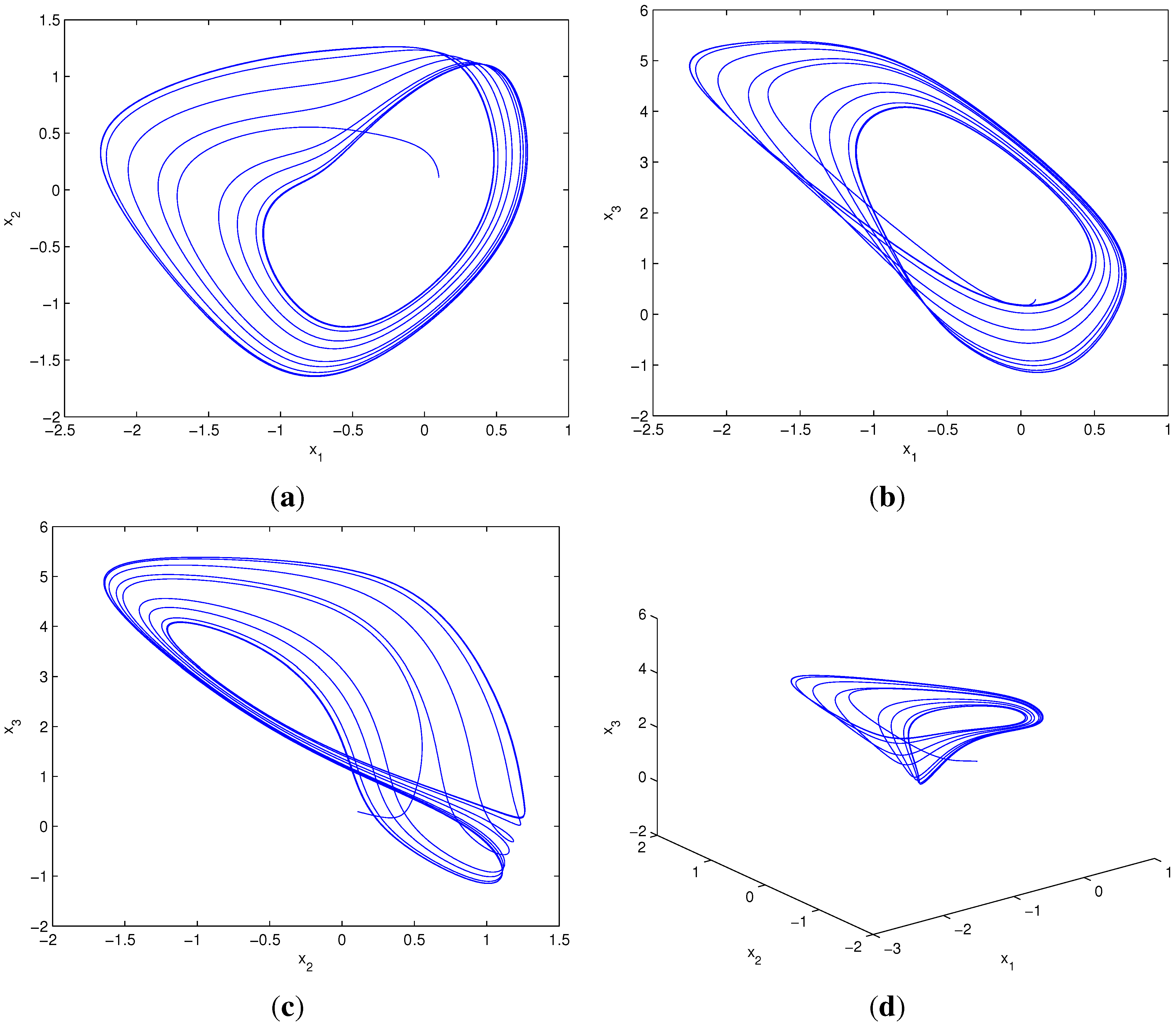
where $x(t)={(x_1(t),x_2(t),x_3(t))}^T$, $C=$diag$(1,1,1)$, $f(x(t))={(tanh(x_1(t)),tanh(x_2(t)),tanh(x_3(t)))}^T$, and $A=\left[\begin{array}{ccc}2& -1.2& 0\\ 2& 1.71& 1.15\\ -4.75& 0& 1.1\end{array}\right]$. The system satisfies Assumption 1 with $L_1=L_2=L_3=1$. As is shown in Figure 1, the fractional-order Hopfield neural network possesses a chaotic behavior when $\alpha =0.95$.

Figure 1. Chaotic behaviors of fractional-order Hopfield neural network Equation (34) with fractional-order, $\alpha =0.95$.

Figure 1. Chaotic behaviors of fractional-order Hopfield neural network Equation (34) with fractional-order, $\alpha =0.95$.

The controlled response fractional Hopfield neural network is designed as follows:

$$\begin{array}{c}\hfill D^{\alpha }y(t)=-Cy(t)+Af(y(t))+u(t)\end{array}$$

(35)

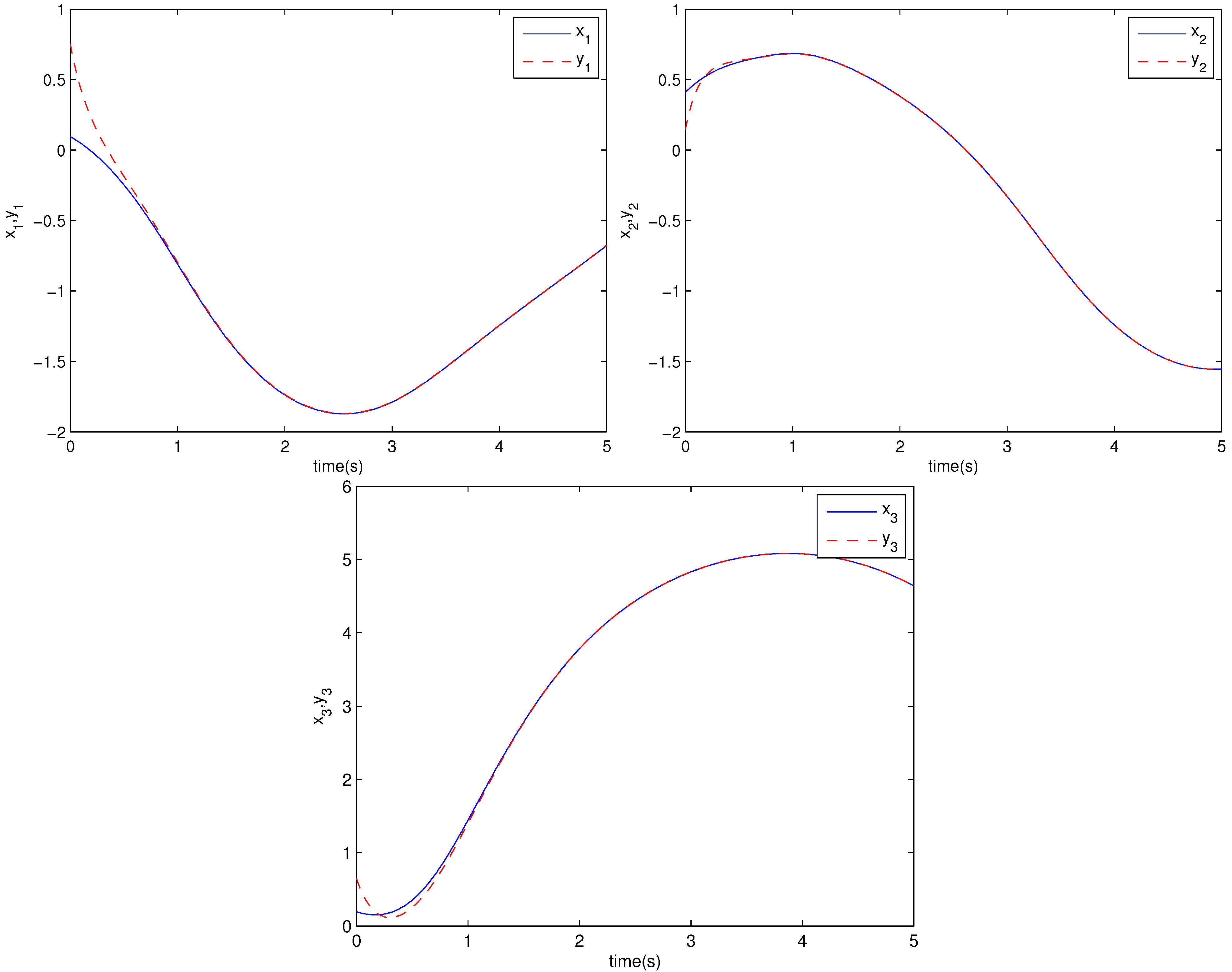
The controller gain matrix, $u(t)$, is chosen as K= diag$(-6,-5,-2)$, and it can be easily verified that $(C-K)-|A|L=$$\left[\begin{array}{ccc}5& -1.2& 0\\ -2& 4.29& -1.15\\ -4.75& 0& 1.9\end{array}\right]$ is an M matrix. According to Theorem 1, the synchronization between Equations (34) and (35) can be achieved. In the numerical simulations, the initial states of the drive and response systems are taken as $x(0)={(0.1,0.4,0.2)}^T$ and $y(0)={(0.8,0.1,0.7)}^T$, respectively. 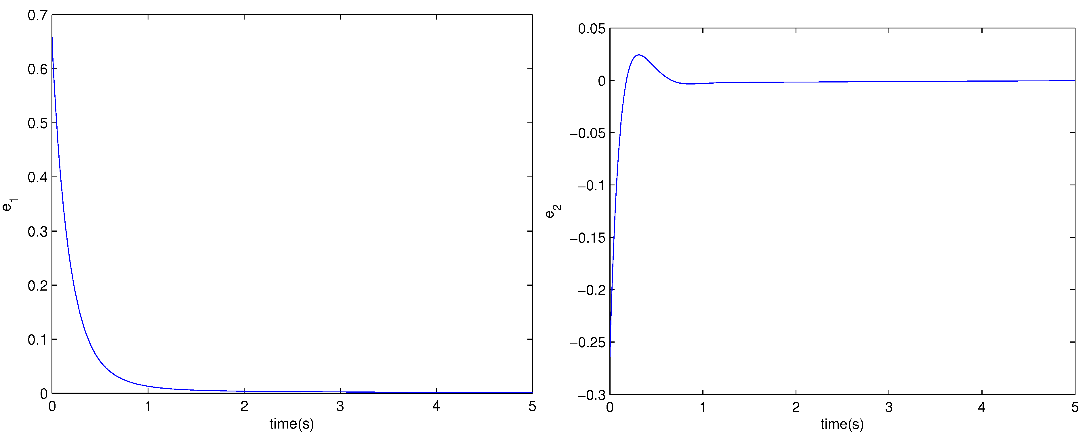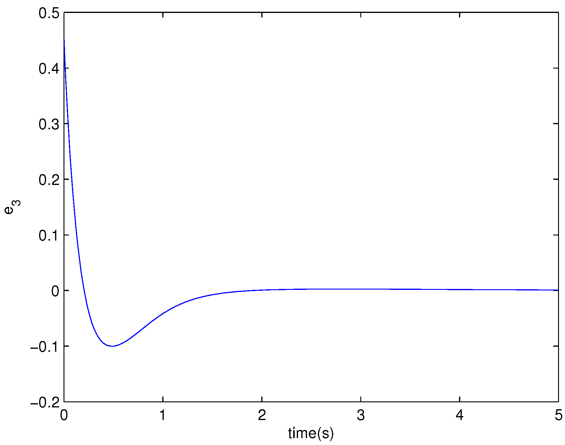Figure 2 shows the state synchronization trajectory of the drive and response systems; the synchronization error response is depicted in Figure 3.

Figure 2. State synchronization trajectories of drive system Equation (34) and response system Equation (35).

Figure 2. State synchronization trajectories of drive system Equation (34) and response system Equation (35).

Figure 3. Synchronization error time response of drive system Equation (34) and response system Equation (35).

Figure 3. Synchronization error time response of drive system Equation (34) and response system Equation (35).

5. Conclusions

In this paper, the synchronization problem has been studied theoretically for a class of fractional-order chaotic neural networks, which is more difficult and challenging than the integer-order chaotic neural networks. Based on the Mittag-Leffler function and linear feedback control, a sufficient condition in the form of the M-matrix has been derived. Finally, a simulation example has been given to illustrate the effectiveness of the developed approach.