Article

On the Topological Entropy of Some Skew-Product Maps

Departamento de Matemática Aplicada y Estadística, Universidad Politécnica de Cartagena, C/ Dr. Fleming sn, 30202 Cartagena, Murcia 30000, Spain
Entropy 2013, 15(8), 3100-3108; https://doi.org/10.3390/e15083100
Submission received: 5 July 2013 / Revised: 25 July 2013 / Accepted: 26 July 2013 / Published: 31 July 2013
(This article belongs to the Special Issue Dynamical Systems)

Abstract

:
The aim of this short note is to compute the topological entropy for a family of skew-product maps, whose base is a subshift of finite type, and the fiber maps are homeomorphisms defined in one dimensional spaces. We show that the skew-product map does not increase the topological entropy of the subshift.

1. Introduction

Let Σ = { 0 , 1 , . . . , k 1 } , and let Σ Z = { ( s n ) : s n Σ } . Consider the shift map, σ : Σ Z Σ Z , given by σ ( s n ) = ( s n + 1 ) . Let A = ( a i j ) be a k × k matrix, where the a i j s are 0 s or 1 s for any i , j { 1 , . . . , k } . A subshift of finite type (SFT in short) is the restriction of σ to the set, A = { ( s n ) Σ Z : a s n s n + 1 = 1 } . Note that A is compact and metrizable and σ ( A ) = A , that is, A is invariant by σ.
Let X be a metric space and consider continuous maps, f 0 , f 1 , . . . , f k 1 : X X . Let φ : A × X A × X be the skew-product map given by:
φ ( ( s n ) , x ) = ( σ ( s n ) , f s 0 ( x ) ) , for all ( ( s n ) , x ) A × X
Recently, this class of skew-product maps has been studied by several authors (see [1,2,3,4,5]). The interest for studying systems that are generated by alternative iterations of a finite number of maps comes from several fields, like population dynamics (see, e.g., [6,7]) and economic dynamics (see, e.g., [8,9]), where the systems are generated by SFT with many finite elements. For SFT with infinitely many elements, the term crazy dynamics was introduced in [1]. Let us also point out that this kind of skew-product has been useful for analyzing difference inclusions used in discrete control systems (see, e.g., [10]).
Recently, in [2], the topological entropy of φ was analyzed when k = 2 and A = { 0 , 1 } Z , proving that when f 0 and f 1 belong to a family of contractive homeomorphisms on the real line, the topological entropy of some invariant set agrees with that of the full shift, σ : { 0 , 1 } Z { 0 , 1 } Z . Additionally, in [3], they extend their results to homeomorphisms on higher dimension spaces. The aim of this paper is to analyze the same question under different conditions. Let h ( f ) and ent ( g ) denote the topological entropy and a variant valid for non-compact spaces introduced in Section 2. The main aim of this paper is to state the following results.
Theorem 1 
Let f 0 , f 1 : X X be homeomorphisms on X = S 1 , [ 0 , 1 ] or R . Let φ : A × X A × X , A { 0 , 1 } Z be the skew-product map defined in Equation (1). Then:
(a) 
If X = S 1 or [ 0 , 1 ] , then h ( φ ) = h ( σ ) .
(b) 
If X = R , then ent ( φ ) h ( σ ) . If there exists a compact subset, K R , such that φ ( A × K ) A × K , then ent ( φ ) = h ( σ ) .
Note that homeomorphisms on the circle, the compact interval and the real line have zero topological entropy, and therefore, one might wonder whether the above result remains true for simple maps, that is, for zero entropy maps. The next result, in the spirit of the dynamic Parrondo paradox (see, e.g., [11,12,13,14]), shows that this is not true in general.
Theorem 2 
Let φ : A × [ 0 , 1 ] A × [ 0 , 1 ] , A { 0 , 1 } Z be the skew-product map defined in Equation (1). Then, there are zero topological entropy continuous maps, f 0 , f 1 : [ 0 , 1 ] [ 0 , 1 ] , such that h ( φ ) > h ( σ ) .
The maps used in the proof of Theorem 2 are constructed by gluing different continuous interval maps, which usually do not appear in discrete models from natural or social sciences. The next result shows that a similar result holds for a well-known one-parameter family of interval maps.
Theorem 3 
Let g a ( x ) = a x ( 1 x ) , a [ 3 , 4 ] and x [ 0 , 1 ] . Fix a , b [ 3 , 4 ] , and let φ : A × [ 0 , 1 ] A × [ 0 , 1 ] , A { 0 , 1 } Z be the skew-product map defined in Equation (1) with f 0 = g a and f 1 = g b . Then, there are parameter values, a 0 , a 1 [ 3 , 4 ] , such that h ( g a ) = h ( g b ) = 0 and h ( φ ) > h ( σ ) for a suitable SFT.
Let us remark that there are a wide ranges of parameters, a [ 3 , 4 ] , satisfying Theorem 3. However, we can give some positive results if we strengthen our hypothesis. Recall that a continuous interval map is piecewise monotone if there are 0 = x 0 < x 1 < . . . < x n = 1 , such that f | ( x i , x i + 1 ) is monotone for i = 0 , . . . , n 1 . Recall that two maps, f 0 and f 1 , commute if f 0 f 1 = f 1 f 0 . Then, we can prove the following result, which gives a partial positive answer to our previous question.
Theorem 4 
Let f 0 , f 1 : [ 0 , 1 ] [ 0 , 1 ] be commuting continuous piecewise monotone with zero topological entropy. Let φ : A × [ 0 , 1 ] A × [ 0 , 1 ] , A { 0 , 1 } Z be the skew-product map defined in Equation (1). Then, h ( φ ) = h ( σ ) .
Remark 1 
Theorem 4 is not true in general if both maps, f 0 and f 1 , are not piecewise monotone. Namely, in [15], two commuting maps, f 0 and f 1 , with zero topological entropy are constructed, such that h ( f 0 f 1 ) > 0 , and so, following the proof of Theorem 3, we can conclude that h ( σ ) < h ( φ ) .
The paper is organized as follows. The next section is devoted to introduce basic notation and useful definitions. Then, we give a proof of Theorem 1. The last section is devoted to proving Theorems 2–4.

2. Basic Definitions

Firstly, we will introduce Bowen’s definition of topological entropy (see [16]). Let X be a compact metric space with metric d, and let f : X X be a continuous map. Let K be a compact subset of X, and fix n N and ε > 0 . A subset, S K , is said to be ( n , ε , K ) -separated if for any x , y S , x y , there is k { 0 , 1 , . . . , n 1 } , such that d ( f k ( x ) , f k ( y ) ) > ε . Denote by s e p n ( ε , K ) the cardinality of an ( n , ε , K ) -separated set with maximal cardinality. The topological entropy is defined as:
h ( f ) = lim ε 0 lim sup n 1 n log s e p n ( ε , X )
We say that a continuous map, f, is topologically chaotic if h ( f ) > 0 . In particular, topologically chaotic maps are chaotic in the sense of Li and Yorke (see [17,18]), which is one of the most accepted notions of chaos. In addition, the topological entropy of the skew-product map, φ, defined in Equation (1), satisfies the following Bowen’s inequalities:
max h ( σ ) , sup ( s n ) A h ( φ , X , ( s n ) ) h ( φ ) h ( σ ) + sup ( s n ) A h ( φ , X , ( s n ) )
where for any ( s n ) A :
h ( φ , X , ( s n ) ) = lim ε 0 lim sup n 1 n log s e p n ( ε , { ( s n ) } × X )
which can be meant as the topological entropy of the non-autonomous discrete system given by the sequence of maps, ( f s 0 , f s 1 , . . . ) (see [19] for the definition).
When X is not compact, the above definition of topological entropy makes sense when f is uniformly continuous. Then, we need to add a new limit in the definition as follows:
h d ( f ) = sup K lim ε 0 lim sup n 1 n log s e p n ( ε , K )
We stress the metric, d, now, because this definition is metric-dependent. However, it is known (see, e.g., [20]) that, although the dynamics of the map, f ( x ) = 2 x , x R , is simple, we have that h d ( f ) = log 2 for the standard Euclidean metric on R . To solve this problem, in [21], a notion of topological entropy for non-compact spaces has been introduced, such that it can be computed for any continuous map and keeps the above property, that positive entropy maps have a complicated dynamic behavior. Denote by K ( X , f ) the family of compact subsets, K of X, such that f ( K ) K , and define:
ent ( f ) = sup K K ( X , f ) lim ε 0 lim sup n 1 n log s e p n ( ε , K )
Note that, clearly, ent ( f ) h d ( f ) , and for f ( x ) = 2 x , we easily see that ent ( f ) = 0 , because the only invariant compact subset is { 0 } . Additionally, ent ( f ) = 0 when K ( X , f ) = .
Now, we concentrate our efforts in proving our main results.

3. Proof of Theorem 1

Proof of case (a). Let f n : X X be a sequence of homeomorphisms with X = S 1 or [ 0 , 1 ] . It can be seen in [19] that if we denote by f 1 , the sequence of maps, ( f 1 , f 2 , . . . . ) , then h ( f 1 , ) = 0 . To finish the proof, we apply Bowen’s inequality (2) to conclude that, since:
sup ( s n ) A h ( φ , X , ( s n ) ) = 0
we have that h ( φ ) = h ( σ ) .
When X = R , we cannot apply Bowen’s inequality, and therefore, the proof requires extra work.
Proof of case (b). Note that R = ( , + ) . We add two symbols to R and construct the compact space, [ , + ] , which is homeomorphic to a compact interval. Since f 0 and f 1 are homeomorphisms, we can extend them continuously and construct maps, f i * : [ , + ] [ , + ] , such that f i * ( ± ) { ± } , i = 0 , 1 . Note that f 0 * and f 1 * are homeomorphisms, as well, and therefore:
h ( f s 0 * , f s 1 * , . . . ) = 0
for all ( s n ) A .
On the other hand, we consider the continuous extension of φ:
φ * : A × [ , + ] A × [ , + ]
given by:
φ * ( ( s n ) , x ) = ( σ ( s n ) , f s 0 * ( x ) ) , for all ( ( s n ) , x ) A × [ , + ]
Since any compact subset of A × ( , + ) is a compact subset of A × [ , + ] , we conclude that:
ent ( φ ) ent ( φ * ) = h ( φ * )
Applying Bowen’s inequality to φ * , we conclude that:
h ( φ * ) h ( σ ) + sup ( s n ) A h ( φ * , [ , + ] , ( s n ) )
and since:
h ( φ * , [ , + ] , ( s n ) ) = h ( f s 0 * , f s 1 * , . . . ) = 0
we conclude that:
ent ( φ ) h ( φ * ) = h ( σ )
Now, we assume that there exists a compact set, K R , such that φ ( A × K ) A × K . Applying Bowen’s inequality to φ | A × K , we conclude that:
h ( σ ) h ( φ | A × K ) ent ( φ )
which concludes the proof.
Remark 2 
The existence of compact subsets, K, holding the conditions of Theorem 1 (b) can be seen in [2,10]. The following example shows that the equality, h ( σ ) = ent ( φ ) , is not true in general when such compact subsets do not exist. We just consider the real maps, f i ( x ) = x + i + 1 , i = 0 , 1 , and construct the map, φ. Clearly K ( Σ Z × R , φ ) = , which implies that ent ( φ ) = 0 . If we take as a base map, σ : A A , with positive topological entropy, then we find that h ( σ ) > h ( φ ) = 0 .

4. Proof of Theorems 2–4

Proof of Theorem 2. Let A = { 0 , 1 } Z , and define the maps, f 0 and f 1 , as follows:
f 0 ( x ) = ( g 2 t 2 g 1 1 ) ( x ) if x [ 0 , 1 / 2 ] 1 / 2 if x [ 1 / 2 , 1 ]
and:
f 1 ( x ) = 1 / 2 if x [ 0 , 1 / 2 ] ( g 1 ϕ t 2 ϕ g 2 1 ) ( x ) if x [ 1 / 2 , 1 ]
where g 1 ( x ) = x / 2 , g 2 ( x ) = ( x + 1 ) / 2 and ϕ ( x ) = 1 x , x R , and t is the standard tent map, t ( x ) = 1 | 2 x 1 | , x [ 0 , 1 ] , which holds that h ( t 2 ) = log 4 . 
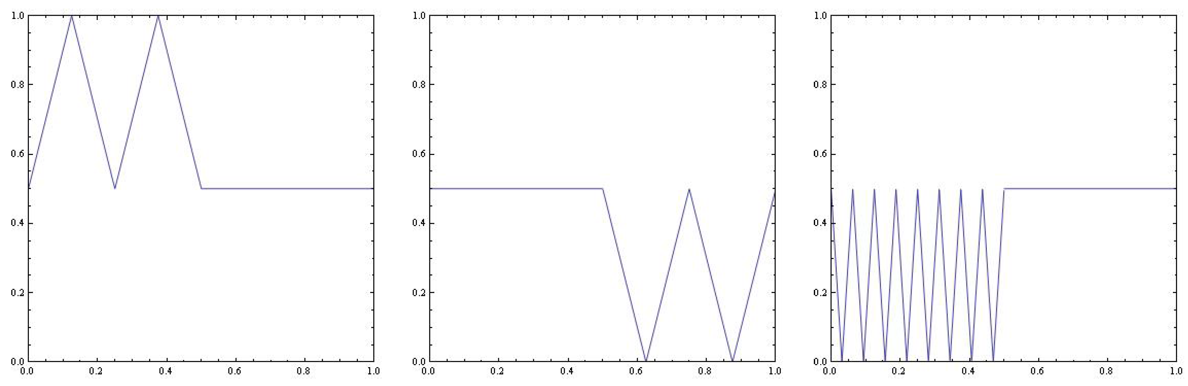
Figure 1 shows the graph of f 0 and f 1 on the interval, [ 0 , 1 ] .
Figure 1. We show the graphic on [ 0 , 1 ] of maps f 0 (left), f 1 (center) and f 1 f 0 (right), defined in the proof of Theorem 2.
Entropy 15 03100 g001
Note that f i 2 ( [ 0 , 1 ] ) = 1 / 2 , i = 1 , 2 , and thus, h ( f 0 ) = h ( f 1 ) = 0 . Let ( 0 , 1 , 0 , 1 , . . . ) A , and note that, by [19]:
h ( φ , [ 0 , 1 ] , ( 0 , 1 , 0 , 1 . . . ) ) = h ( f 0 , f 1 , f 0 , f 1 , . . . ) = 1 2 h ( f 1 f 0 )
On the other hand, we have that:
( f 1 f 0 ) ( x ) = ( g 1 ϕ t 4 ϕ g 1 1 ) ( x ) if x [ 0 , 1 / 2 ] 1 / 2 if x [ 1 / 2 , 1 ]
whose graphic can be seen in Figure 1. By [22], h ( f 1 f 0 ) = log 16 . By Bowen’s inequalities:
h ( φ ) h ( φ , [ 0 , 1 ] , ( 0 , 1 , 0 , 1 . . . ) ) = log 4 > log 2 = h ( σ )
and the proof concludes.
Proof of Theorem 3. Let f a ( x ) = a x ( 1 x ) , a [ 3 , 4 ] and x [ 0 , 1 ] . It is well-known that h ( f a ) increases when a increases (see, e.g., [23]), and it is positive for a > 3.5699 . . . 
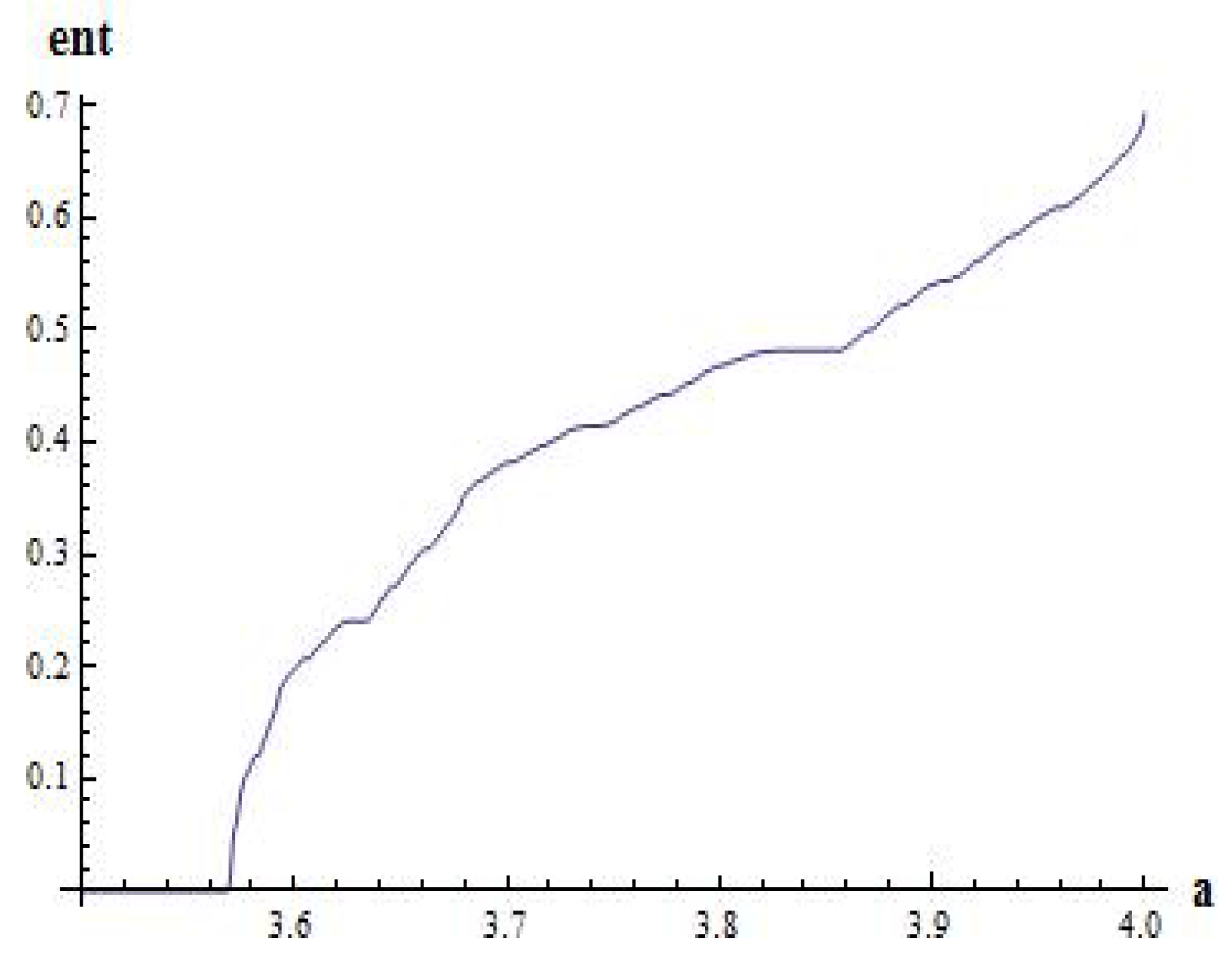
Figure 2 shows the computation of h ( f a ) with accuracy 10 4 by using an algorithm from [24]. However, for f a f b , a , b [ 3 , 4 ] , the computation of topological entropy with prescribed accuracy is more complicated. For doing it, we use the recently developed algorithm from [25]. 
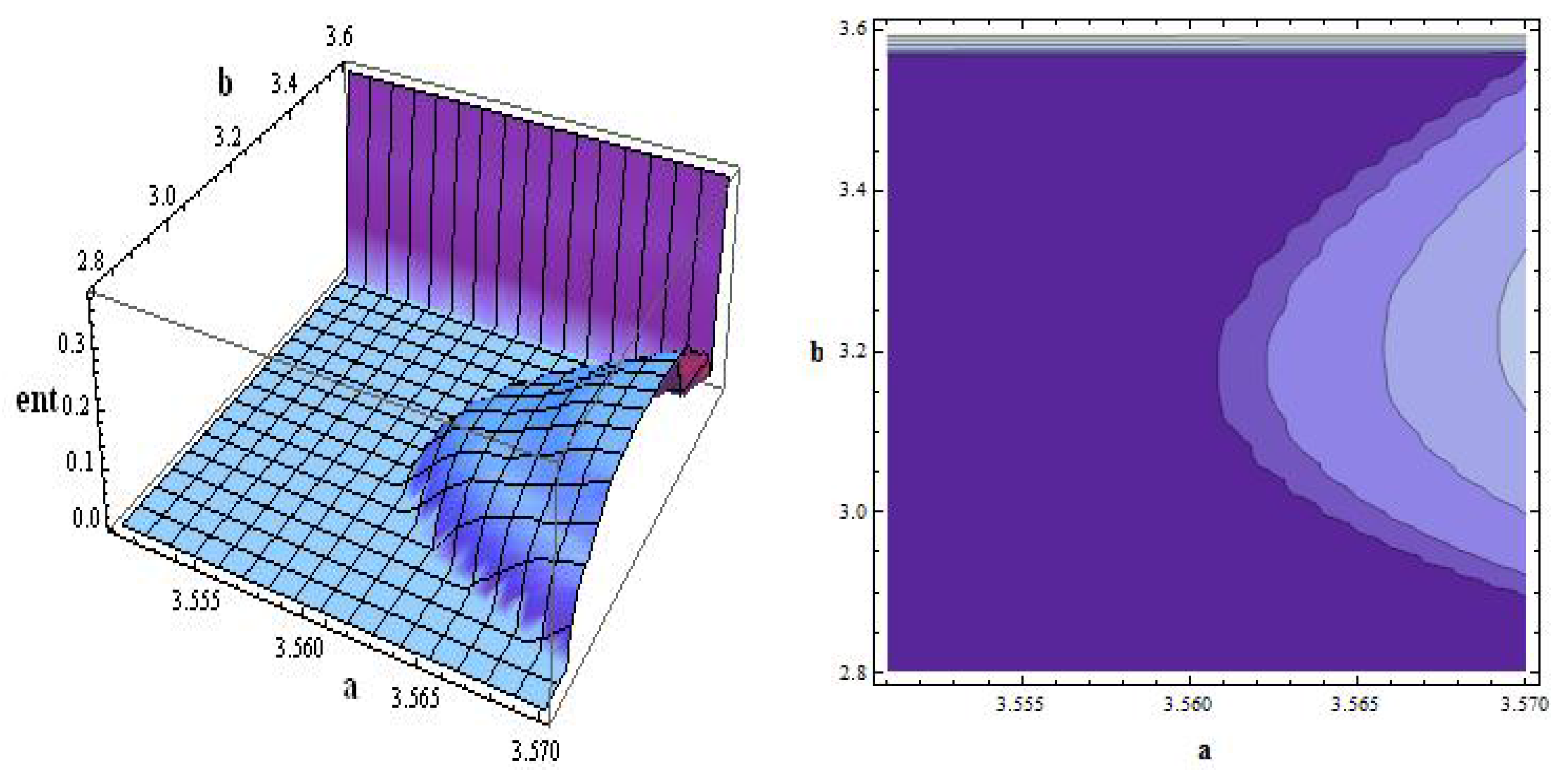
Figure 3 shows the entropy computations with prescribed accuracy, 10 4 . From the shown computations, we may find parameter values, a and b, a bit smaller than 3.6 with zero topological entropy for maps f a and f b , such that h ( f a f b ) is positive (for instance, a = 3.56 and 3.086 b 3.267 gives positive values of h ( f a f b ) ).
Figure 2. We compute the topological entropy (ent in the figure) for a [ 3.5 , 4 ] with accuracy, 10 4 . We note that the first parameter value providing positive topological entropy is 3.569945 . . .
Entropy 15 03100 g002
Figure 3. We compute the topological entropy (ent in the figure) for a [ 3.55 , 3.57 ] and b [ 2.8 , 3.6 ] with accuracy, 10 4 . The darker region represents those parameter values providing zero topological entropy.
Entropy 15 03100 g003
Now, we consider the matrix:
A = 0 1 1 0
and notice that the SFT, σ : A A , generated by A is composed of two periodic sequences, ( 0 , 1 , 0 , 1 , . . ) and ( 1 , 0 , 1 , 0 , . . . ) , which implies that h ( σ ) = 0 . On the other hand, if f 0 = f a and f 1 = f b , notice that:
h ( φ , X , ( 0 , 1 , 0 , 1 , . . . ) ) = h ( f 0 , f 1 , f 0 , f 1 , . . . ) = 1 2 h ( f 1 f 0 ) h ( φ , X , ( 1 , 0 , 1 , 0 , . . . ) ) = h ( f 1 , f 0 , f 1 , f 0 , . . . ) = 1 2 h ( f 0 f 1 )
It is easy to check that:
h ( φ ) = 1 2 h ( f 0 f 1 ) = 1 2 h ( f 1 f 0 ) > 0 = h ( σ )
which concludes the proof.
Proof of Theorem 4. Let c ( f ) denote the number of monotonicity pieces of a piecewise monotone map, f. By the Misiurewicz-Szlenk (see [22]) formula:
h ( f ) = lim n 1 n log c ( f n )
Fix ( s n ) A and note that:
c ( f s n 1 f s n 2 . . . f s 0 ) = c ( f 1 k n f 0 n k n ) c ( f 1 k n ) c ( f 0 n k n )
where k n = # { i { 0 , 1 , . . . , n 1 } : s i = 1 } . Since the sequence, ( f s 0 , f s 1 , . . . ) , contains two maps, it is equicontinuous, and then, the Misiurewicz-Szlenk formula is valid in this setting (see [26]). Thus:
h ( f s 0 , f s 1 , . . . ) = lim sup n 1 n log c ( f s n 1 f s n 2 . . . f s 0 ) lim sup n k n n 1 k n log c ( f 1 k n ) + lim sup n n k n n 1 n k n log c ( f 0 n k n ) h ( f 1 ) lim sup n k n n + h ( f 0 ) lim sup n n k n n
and since h ( f 0 ) = h ( f 1 ) = 0 , we find that for any ( s n ) A , we have that h ( f s 0 , f s 1 , . . . ) = 0 . By Bowen’s inequality:
h ( φ ) h ( σ ) + sup ( s n ) A h ( f s 0 , f s 1 , . . . ) = h ( σ )
Since the inequality, h ( σ ) h ( φ ) , also holds, we conclude the proof.

5. Conclusions

We prove that skew-product maps with the form of Equation (1), such that the fiber maps are homeomorphisms on one dimensional spaces, do not increase the topological entropy of its base map, and then, the behavior of the space, X, is not dynamically complicated, generalizing a result from [2]. On the other hand, we also prove that a similar situation does not hold when zero topological entropy continuous interval maps are considered. Still, the question remains open of whether our results can be extended to homeomorphisms defined on topological spaces with dimensions greater than one.

Acknowledgments

This paper has been partially supported by the grants, MTM2011-23221, from Ministerio de Ciencia e Innovación (Spain) and 08667/PI/08 from Programa de Generación de Conocimiento Científico de Excelencia de la Fundación Séneca, Agencia de Ciencia y Tecnología de la Comunidad Autónoma de la Región de Murcia (II PCTRM 2007–10).

Conflict of Interest

The author declares no conflict of interest.

References

  1. Afraimovich, V.S.; Shilnikov, L.P. Certain global bifurcations connected with the disappearance of a fixed point of saddle-node type. Dokl. Akad. Nauk. SSSR 1974, 214, 1281–1284. [Google Scholar]
  2. Amigó, J.M.; Kloeden, P.E.; Giménez, A. Switching systems and entropy. J. Differ. Equ. Appl. 2013. [Google Scholar] [CrossRef]
  3. Amigó, J.M.; Kloeden, P.E.; Giménez, A. Entropy increase in switching systems. Entropy 2013, 15, 2363–2383. [Google Scholar] [CrossRef]
  4. Cánovas, J.S.; Falcó, A. The set of periods for a class of skew-products. Discret. Contin. Dyn. Syst. 2000, 6, 893–900. [Google Scholar]
  5. Falcó, A. The set of periods for a class of crazy maps. J. Math. Anal. Appl. 1998, 217, 546–554. [Google Scholar] [CrossRef]
  6. Cushing, J.; Henson, S. The effect of periodic habit fluctuations on a nonlinear insect population model. J. Math. Biol. 1997, 36, 201–226. [Google Scholar]
  7. Jillson, D. Insect population respond to fluctuating environments. Nature 1980, 288, 699–700. [Google Scholar] [CrossRef]
  8. Matsumoto, A.; Nonaka, Y. Statistical dynamics in chaotic cournot model with complementary goods. J. Econ. Behav. Organ. 2006, 61, 769–783. [Google Scholar] [CrossRef]
  9. Puu, T. Chaos in duopoly pricing. Chaos Solitons Fractals 1991, 1, 573–581. [Google Scholar] [CrossRef]
  10. Cheban, D. Compact global chaotic attractors of discrete control systems. Nonautonomous Stochastic Dyn. Syst. 2013. [Google Scholar] [CrossRef]
  11. Almeida, J.; Peralta-Salas, D.; Romera, M. Can two chaotic systems give rise to order? Phys. D 2005, 200, 124–132. [Google Scholar] [CrossRef]
  12. Cánovas, J.S.; Linero, A.; Peralta-Salas, D. Dynamic Parrondo’s paradox. Phys. D 2006, 218, 177–184. [Google Scholar] [CrossRef]
  13. Harmer, G.P.; Abbott, D. Parrondo’s paradox. Stat. Sci. 1999, 14, 206–213. [Google Scholar]
  14. Parrondo, J.M.R.; Harmer, G.P.; Abbott, D. New paradoxical games based on Brownian ratchets. Phys. Rev. Lett. 2000, 85, 5226–5229. [Google Scholar] [CrossRef] [PubMed]
  15. Raith, P. Two commuting interval maps with entropy zero whose composition has positive topological entropy. Grazer Math. Ber. 2004, 346, 351–354. [Google Scholar]
  16. Bowen, R. Entropy for group endomorphism and homogeneous spaces. Trans. Am. Math. Soc. 1971, 153, 401–414. [Google Scholar] [CrossRef]
  17. Blanchard, F.; Glasner, E.; Kolyada, S.; Maass, A. On Li-Yorke pairs. J. Reine Angew. Math. 2002, 547, 51–68. [Google Scholar] [CrossRef]
  18. Li, T.Y.; Yorke, J.A. Period three implies chaos. Am. Math. Mon. 1975, 82, 985–992. [Google Scholar] [CrossRef]
  19. Kolyada, S.; Snoha, L. Topological entropy of nonautononous dynamical systems. Random Compet. Dyn. 1996, 4, 205–233. [Google Scholar]
  20. Walters, P. An Introduction to Ergodic Theory; Springer Verlag: New York, NY, USA, 1982. [Google Scholar]
  21. Cánovas, J.S.; Rodríguez, J.M. Topological entropy of maps on the real line. Topol. Appl. 2005, 153, 735–746. [Google Scholar] [CrossRef]
  22. Misiurewicz, M.; Szlenk, W. Entropy of piecewise monotone mappings. Stud. Math. 1980, 67, 45–63. [Google Scholar]
  23. de Melo, W.; van Strien, S. One-Dimensional Dynamics; Springer-Verlag: Berlin, Germany, 1993. [Google Scholar]
  24. Block, L.; Keesling, J.; Li, S.; Peterson, K. An improved algorithm for computing topological entropy. J. Stat. Phys. 1989, 55, 929–939. [Google Scholar] [CrossRef]
  25. Cánovas, J.S.; Muñoz, M. Computing topological entropy for periodic sequences of unimodal maps. 2012; in press. [Google Scholar]
  26. Kolyada, S.; Misiurewicz, M.; Snoha, L. Topological entropy of nonautonomous piecewise monotone dynamical systems on the interval. Fund. Math. 1999, 160, 161–181. [Google Scholar]

