Article

Spatially-Explicit Bayesian Information Entropy Metrics for Calibrating Landscape Transformation Models

1
Institute for Geocomputational Analysis and Statistics (GeoCAS), University of the Virgin Islands, 2 John Brewer's Bay, St. Thomas, VI 00802, USA
2
Department of Computer and Computational Sciences, College of Science and Mathematics, University of the Virgin Islands, 2 John Brewer's Bay, St. Thomas, VI 00802, USA
3
Department of Forestry and Natural Resources, Purdue University, West Lafayette, IN 47906, USA
*
Author to whom correspondence should be addressed.
Entropy 2013, 15(7), 2480-2509; https://doi.org/10.3390/e15072480
Submission received: 2 May 2013 / Revised: 9 June 2013 / Accepted: 13 June 2013 / Published: 25 June 2013
(This article belongs to the Special Issue Entropy and Urban Sprawl)

Abstract

:
Assessing spatial model performance often presents challenges related to the choice and suitability of traditional statistical methods in capturing the true validity and dynamics of the predicted outcomes. The stochastic nature of many of our contemporary spatial models of land use change necessitate the testing and development of new and innovative methodologies in statistical spatial assessment. In many cases, spatial model performance depends critically on the spatially-explicit prior distributions, characteristics, availability and prevalence of the variables and factors under study. This study explores the statistical spatial characteristics of statistical model assessment of modeling land use change dynamics in a seven-county study area in South-Eastern Wisconsin during the historical period of 1963–1990. The artificial neural network-based Land Transformation Model (LTM) predictions are used to compare simulated with historical land use transformations in urban/suburban landscapes. We introduce a range of Bayesian information entropy statistical spatial metrics for assessing the model performance across multiple simulation testing runs. Bayesian entropic estimates of model performance are compared against information-theoretic stochastic entropy estimates and theoretically-derived accuracy assessments. We argue for the critical role of informational uncertainty across different scales of spatial resolution in informing spatial landscape model assessment. Our analysis reveals how incorporation of spatial and landscape information asymmetry estimates can improve our stochastic assessments of spatial model predictions. Finally our study shows how spatially-explicit entropic classification accuracy estimates can work closely with dynamic modeling methodologies in improving our scientific understanding of landscape change as a complex adaptive system and process.

Graphical Abstract

1. Introduction

The transformation of landscapes by humans is well known to be a complex phenomenon directed by a host of socioeconomic drivers interacting at multiple spatial and temporal scales [1]. The spatial patterns of land use land cover that result from human activity on the landscape are in turn complex and very heterogeneous [2]. In many ways, the process and patterns inherent in landscape transformations can be viewed as stochastic. Understanding landscape transformation is considered one of the eight grand challenges in environmental research [3] as changes in land use land cover affect a variety of environmental parameters, such as water quality [4], hydrologic [5] and hydroclimatic [6] dynamics, energy balances at the land-atmosphere boundary [7], local and regional climate patterns [8], biodiversity [9], and biogeochemical cycles [10]. Thus understanding landscape transformations is important to developing predictive tools that can be used to determine environmental impacts of future landscape transformations.
Unfortunately, traditional statistical accuracy assessment techniques of land change models, although essential for validating observed and historical land use changes, fail to capture the stochastic character of the dynamics that are simulated [11], especially across multiple scales. Here, we propose new metrics and indicators that provide the modeler the ability to extract higher-order information dynamics from landscape transformation simulations. Previous work in landscape transformation simulation assessment has focused on simple contingency table metrics that measure the relative differences of true positive, false positive, true negative and false negative locations [12,13,14], measures of correct quantity of change [11], the pattern of change [13], and/or the relative cost of errors across the simulation domain [8]. Although much progress has been made in this area in the last decade, it is also well recognized that adequate measures of the simulation itself and model output still need development [15].
The research presented here provides a detailed guide for assessing the level of entropy of model simulations of landscape transformation. The term information entropy, originates from the information-theoretic concept of entropy, conceived by Claude Shannon on his famous two articles of 1948 in Bell System Technical Journal [16], and expanded later in his book “Mathematical Theory of Communication” [17]. Since the mid-20th century, the field of information theory has experienced an unprecedented development, especially following the expansion of computer science in almost every scientific field and discipline. The concept of entropy in information systems theory allow us to allocate quantitative measurements of uncertainty contained within a random event (or a variable describing it) or a signal representing a process [18,19]. The literature on assessing spatially explicit models of landscape transformation has made substantial steps during the last few years. Many of the metrics and assessment techniques in the past have been treating land use predictions as complex signals, and models themselves often are treated as measurement instruments, not different from signal-measurement devise assessment in physics experiments [20]. Spatially explicit methods and assessment techniques are used in many remote sensing applications [21], wildlife habitat models [22], predicting presence, abundance and spatial distribution of animal populations [23], and analyzing the availability and management of natural resources [24,25]. In a more theoretical level of analysis, spatially explicit methods of model assessment have been used for testing hypotheses in landscape ecological models [26,27], addressing statistical issues of uncertainty in modeling [25], or analyzing landscape-specific characteristics and spatial distributions [28].
Methodologies and techniques as the ones referenced above often maintain and preserve traditional statistical approaches to model assessment. Most likely, they test the limitations and assumptions of statistical techniques originally designed for analyzing data and variables that do not exhibit spatially explicit variation. The majority of studies where spatially explicit methodologies are used most often involve relatively simple or linear statistical analyses [29,30], albeit some recent studies have incorporated entropy-based statistical considerations in land use transition modeling analyses before [31]. While in recent years the assessment of model complexity has been an issue of analysis [32,33], studies have yet to include spatial complexity and assessment of stochasticity as an essential element of evaluation and analysis. We argue that spatial complexity by itself is not often enough to fully describe and represent the complex system dynamics of coupled human and natural systems. The introduction of spatial complexity in advanced dynamic modeling environments requires the consideration of stochasticity as an essential element of the modeling approach—balancing traditional spatial assessment and game-theoretic approaches to modeling. The level of uncertainty and incomplete information embedded in the components of a coupled natural human—systems often necessitates the introduction of stochasticity as a measurable dimension of complexity [34,35]. Stochastic modeling is widely used in simulating complex natural and ecological phenomena [36], population dynamics [37], spatial landscape dynamics [38], intelligence learning and knowledge-based systems [39], economic and utility modeling [40,41], decision-making, Bayesian and Markov modeling [42,43] and many other associated fields in science and engineering applications but has yet to be applied in landscape transformation modeling
A natural extension of the related techniques and methodologies would be the development and introduction of spatially explicit, stochastic methods of accuracy assessment for simulating complex phenomenon. In recent years, methods, techniques, and measures of informational entropy exceed the single dimensionality of traditional statistical techniques (i.e., measuring uncertainty of single random events or variables) and will research moving to analyzing multi-dimensional signals. Furthermore, applying the techniques of spatial entropy [44,45] will allow landscape transformation modelers to analyze entropy patterns in two-dimensional space. Within these lines, we introduce a case study of land use change in the South-Eastern Wisconsin region, and compare the historical empirical data with simulations. We argue that estimating and interpreting the results of a stochastic model is not simply a question of model calibration, but should incorporate considerations of stochasticity and specificity of the historical and predicted datasets used for the analysis. The spatiotemporal distribution and frequency of the events under study (i.e., land use change transitions), require study of the prior and posterior informational context and content under which those transitions occur and emerge. For example, issues of spatial emergence [46,47], residential urban and suburban locational patterns of development [48,49,50,51], alternative scenarios and trajectories of spatial change [52,53], etc., provide some insight on the multitude of dimensionality and stochasticity embedded within the complex coupled human-environmental system of interactions related to landscape transformation.
The analysis provided in this paper aims to provide a suite of spatially explicit metrics that go beyond traditional statistical calibration and parameter estimation of model predictions, but attempts to provide a statistically sound and comprehensive insight into information-theoretic aspects of the modeled phenomena under study, and explore the parameter space and confines of our predictions. We will show that often it is not enough to ask how well a certain model predicts historical transitions, but we need to determine how well our posterior model estimations are performing given our prior information and ability to predict such transformations.

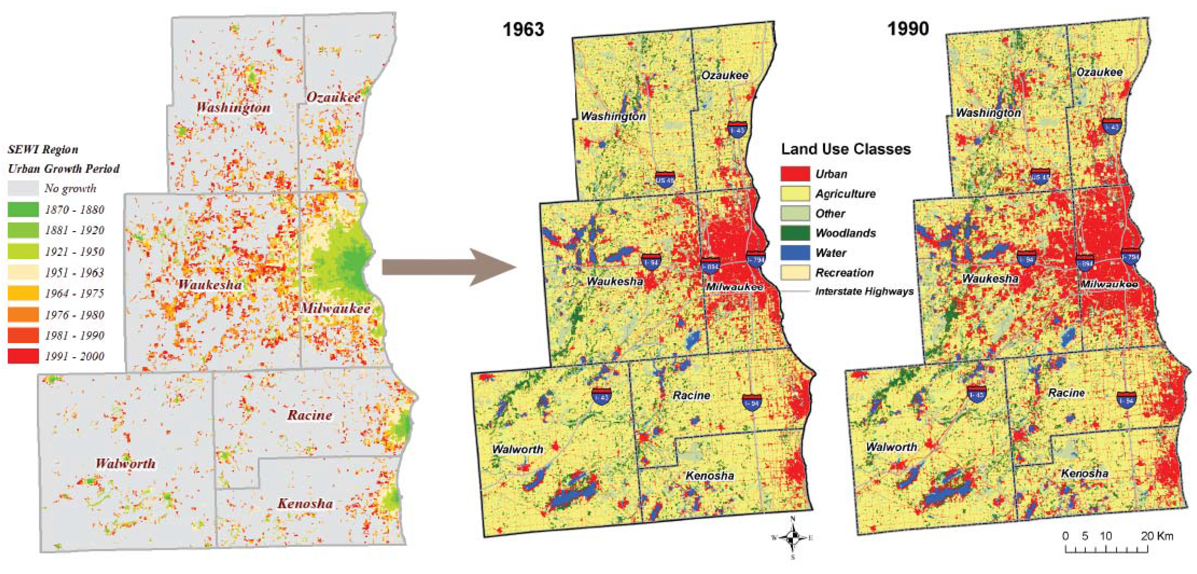
2. Case Study Description

The study presented here is based on simulating historical urban spatial dynamics using Artificial Neural Network (ANN) tools applied to a large metropolitan area of South-Eastern Wisconsin (SEWI) located in the Midwest U.S.A The details of the simulation can be found in a recent paper by Pijanowski et al. [14], where the modeling dynamics and a comprehensive description of the LTM modeling mechanism and experimental design is deployed. The nature of landscape transformations is described in Pijanowski and Robinson [2]. Description of the LTM model is also provided in Pijanowski et al. [13,54,55].

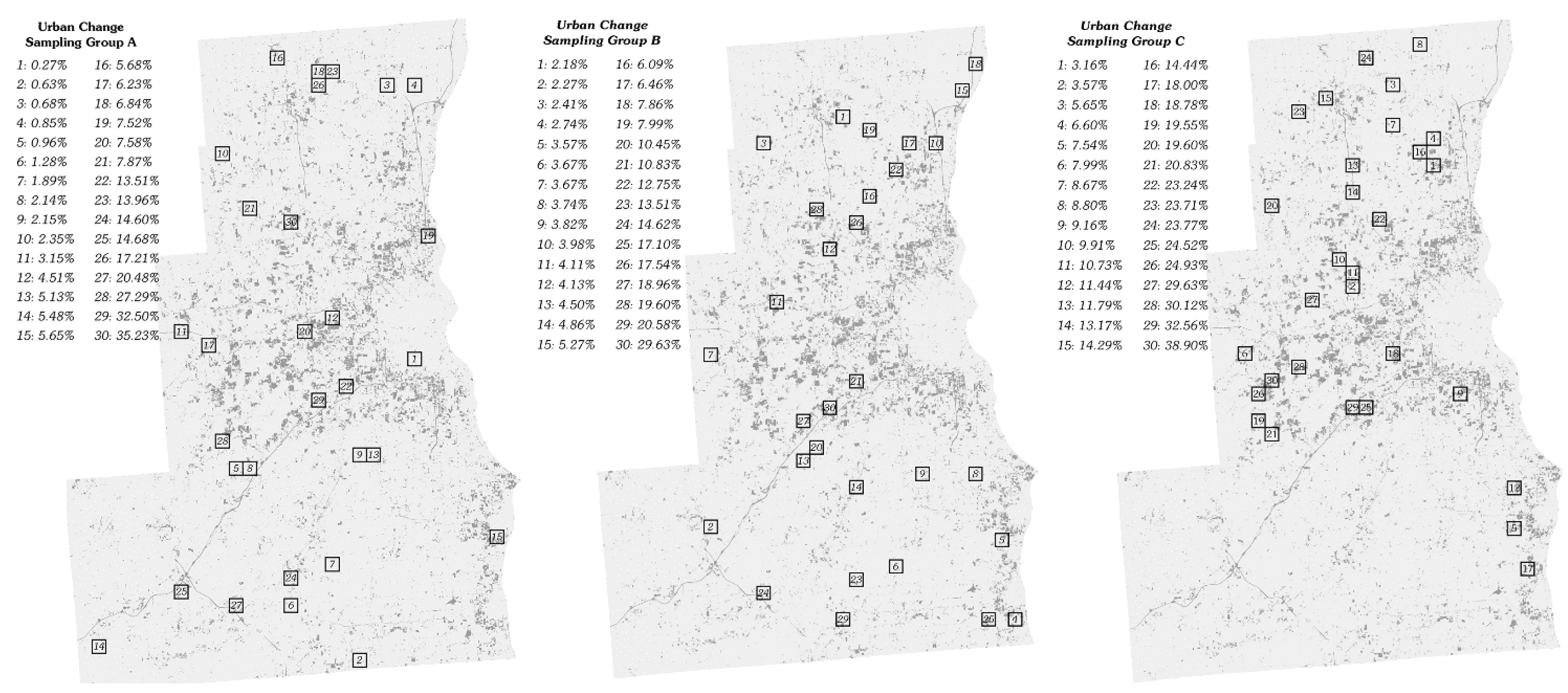
2.1. Sampling Methodology

The SEWI project area includes the city of Milwaukee and its wider suburban area [56]. The land use changes that occurred in the SEWI region during the period 1963–1990 are considerable. Most urban growth has taken place in the suburban metropolitan Milwaukee region, and the areas around medium and large cities in the region (Figure 1). The county of Waukesha, located in the west side of the city of Milwaukee, has witnessed the majority of suburban changes, but highly scattered urban and suburban changes have occurred in the remaining counties both to the north (Washington and Ozaukee counties) and south (Walworth, Racine and Kenosha counties) of the city of Milwaukee. The large size of the area under study, and the enormous differences in rates of urban change allows us to test the ability to perform extensive training and learning simulations using the LTM applied across a range of areas experiencing different urbanization rates To address this test of the robustness of our approach, a comprehensive sampling methodology has been implemented (see also Pijanowski et al. in review). The regional extent of the SEWI area was divided into equal-area square boxes of 2.5 square kilometers (or 6,889 cells of 30 m2 resolution). The square sampling boxes vary in both the number of cells that experienced urban change during the 1963–1990 period, and the amount of exclusionary land zones (urban zones in 1963, paved roads, water bodies, protected areas, etc.). Both parameters affect the modeling performance and the ability to assess comparatively the accuracy of the modeling predictions.
Figure 1. Historical urban changes (1870–2000) and land use changes in the SEWI region, 1963–1990.
Entropy 15 02480 g001
While statistical techniques can be used to model specific exclusionary zoning, as within a Markov transition probability framework, such as the one proposed by Sun et al. [31], the LTM modeling framework [57] treats such zones as external to the analysis and uses a form of masking layer to achieve such exclusion. Theoretically, such exclusionary zones can become subject to urban transitions if their exclusionary properties are lifted (e.g., rezoning transportation areas or roads), yet, such transitions are unlikely to happen within the modeling timeframe, and consequently unlikely to be part of urban planning. A random sampling scheme was implemented for this modeling exercise ensuring comparative assessment of the quantities and spatial patterns of land use change in the region. This approach involved the following steps. First, the regional sampling boxes were ranked and classified using a combined index of both the proportion of urban change and the proportion of exclusionary zone within the sampling box. The resultant combined ranking index takes into account both changes within the sampled boxes and represents the ratio between the percentage of urban change and the percentage of variation in exclusionary zone areas (note that in the LTM, an exclusionary zone is defined as the map area where model pattern training and simulation are not implemented, i.e., these are areas that are not candidates for landscape transformation. Examples of these zones include map areas that are already in non-transitional uses, such as current urban, road and transportation system extents; preserved natural areas, etc.), across the sampled boxes:
Entropy 15 02480 i001
where s = the number of area sampling boxes in the landscape.
From the continuous sampling index values derived from the previous step, two threshold values of the sampling index were used to define three classification index regions for random sampling. The sampling boxes were placed into three sequential classification pool groups (group A, B and C), according to the following rules (thresholds):
Entropy 15 02480 i002
The sampling pool classification in Equation (2) follows a nested hierarchical scheme, that is, the prospective sampling pool of each consequent group is contained in the previous one (i.e., sampling pool for group C is fully contained in group B’s sampling pool, and sampling pool for group B is fully contained within group A’s sampling pool). Such a classification scheme allows the testing of the effects of increased exclusionary zone area to the model performance in the simulations. Sampling pool group A contains all boxes in the sampling region. Sampling pool group B contains only sampling boxes that have no more than double the percentage of exclusionary area than the percentage of urban change area. Finally, sampling pool group C contains only the sampling boxes that have no more than equal or more percentage of urban change area than exclusionary zone area within them. The members (sampling boxes) of each sampling pool group (A, B, and C) have been ranked and assigned to the 30th percentile according to their ascending proportion of urban change within the sample box. From each 30-tile, one sampling box was randomly selected using a random number generator algorithm. The seed of the random number generator was renewed before each sampling operation. The final outcome of the random sampling procedure was three sampling groups (varying on the ascending ratio of urban to exclusionary zone area), containing thirty 2.5 square kilometer sampling boxes each (varying on the percent of urban change), shown in Figure 2 below:
Figure 2. SEWI random sampling groups A, B and C.
Entropy 15 02480 g002

2.2. Simulation Modeling Parameterization

The LTM model requires three levels of parameterization: (a) the simulation drivers of land use change; (b) the training and testing neural network pattern creation; and, (c) the network simulation parameter definition. Details on the theoretical neural network simulation parameterization of the LTM are reported in the literature by Pijanowski et al. [13,54]. Explicit description of the modeling enterprise in the SEWI region are also reported in the Pijanowski et al. [14] paper. In short, eight simulation distance drivers of land use change have been used to parameterize the LTM simulations (urban land in 1963, historical urban centers in 1900, and distance to rivers, lakes and water bodies, highways, state and local roads, and Lake Michigan). The simulation model uses every other cell (50% of the cells) as neural network training pattern, and the entire region for network model testing. Finally, the network is trained for 500,000 training cycles by resetting and iterating the network node’s weight configuration every 100 training cycles, and outputting the network node structure and the mean square error of the network convergence every 100 cycles in a file. Thus for each of the 90 sampled boxes, the simulation output a total of 5,000 network files and MSE values for a grand total of 450,000 simulation result files. For simplicity of presentation, in each of the sampled boxes, forty-four of these network output files are selected for visualization of the results. Due to the nature of the neural network learning dynamics, learning patterns follow a negative exponential increase through training iterations. Thus, a negative exponential scale has been chosen to visualize the results (more frequent samples in lower network training cycles, less frequent samples in higher training cycles).
The simulation results for urban change predictions in 1990 are assessed against historical land use changes in 1990 from existing data provided by the Southeastern Wisconsin Regional Planning Commission [56].

3. Simulation Accuracy Assessment Methodology

The paper by Pijanowski et al. [14] reports three relative conventional statistical metrics for the quantitative accuracy assessment of the model performance. Namely, the percent correct metric (PCM), the Kappa metric (K), and the area under the receiver operator characteristic curve (AROC) metric. The PCM metric is a simple proportional measure of comparison, while the K and AROC metrics take into account the confusion matrix and the omission and commission errors of the simulation. In addition to these conventional metrics (the discussion involving these three metrics is largely omitted from this paper. The reader can consult the corresponding literature, and the Pijanowski et al. paper [14] for more information. Only their value and performance for the simulation experiments in the SEWI region will be reported) three alternative sets of metrics are presented here. The first complementary set is the diagnostic odds ratio for positive (predicted change) and negative (predicted no change), the second complimentary set are the Bayesian predictive value of a positive and negative classification (PPV and NPV) metrics, and the third set is what we call the Bayesian conversion factor (Cb) metric, combined the second set using several estimation criteria. These alternative sets of metrics measure a stochastic level of information entropy (hereafter simply as entropy) in the simulated land use change system. They represent different aspects or dimensions of the predictive value of entropy embedded in the simulation model results, and thus, can enhance our understanding of inherent simulation dynamics and the entropy of spatial patterns resulting from land transformation (Figure 3).
Figure 3. An overview of the analysis sequence process provided in this study. The value of the spatial accuracy assessment and the reduction in classification uncertainty increases from left to right.
Entropy 15 02480 g003

3.1. Basic Definitions

Spatial accuracy assessment requires three major assumptions. The first assumption focusses on the underlying process being simulated. In any given landscape, two theoretical observers (e.g., a simulation model and an observed historical map, or a simulation model and another simulation model, or an observed historical map and an alternative historical map) are assumed to be observed properties of the same underlying process (i.e., represent “real” land transformation). The second assumption is based on the observers themselves. Observers are assumed to face a theoretical level of uncertainty (regardless the degree of, small or large). A simulation model is facing uncertainty on its predicted landscape as a part of the problem formulation (and thus a trivial assumption), but observed historical landscapes are also subject to an implicit degree of uncertainty (i.e., measurement errors, remote sensing classification errors, etc.). These degrees of uncertainty are also not necessarily equal between the two observers. The third assumption involves the assessment process itself. It assumes that the two observers acquire their observations (classification) independently from each other. In other words, the historically observed land use map and the simulation results are independent (or, the modeling predictions are not a function of the real change in the maps). The independence assumption is easy to determine in the case of assessing a simulated and an observed landscape, but it becomes nontrivial when non-parametric analysis is used to compare two modeled landscapes, in cases where the same model with a different configuration is used.
The parametric approximation of spatial accuracy assessment is based on the confusion matrix [58,59] shown in Table 1. For binary land use changes (i.e., presence-absence of a transition), the confusion matrix becomes a 2 × 2 square matrix with exhaustive, and mutually exclusive elements.
Table 1. Confusion matrix for binary spatial accuracy assessment. Simulated versus historical land use change (TN: true negative, TP: true positive, FN: false negative, FP: false positive, SN: simulated negative, SP: simulated positive, RN: real negative, RP: real positive, GT: grand total)
Observed
Simulated 01
0TNFNSN
1FPTPSP
RNRPGT
A nonparametric approximation of spatial accuracy assessment employs the use of the confusion matrix in somewhat more complex forms. It assesses the sensitivity coefficient as the observed fraction of agreement between the two assessed landscapes, or, in other words, the probability of correctly predicting a transition when this transition actually occurred in the observed historical data. Symbolically (S = simulated, R = real):
Entropy 15 02480 i003
Similarly, the specificity coefficient in Equation (4) represents the observed fraction of agreement between two assessed maps, or, in other words, the probability of correctly predicting the absence of transition, when this transition is absent from the historically observed data. Symbolically:
Entropy 15 02480 i004
A theoretically perfect agreement between the two observers would require that:
Entropy 15 02480 i005
The degree of deviation from the rule as defined in Equation (5), represents the degree of deviation from a perfect agreement between the two classifications, or the degree of disagreement between a modeled (simulated) and an observed (historical) landscape transition. The theory of statistical probabilities suggests that a random (fully uncertain) classification between the probabilities denoted by sensitivity and specificity coefficients would be:
Entropy 15 02480 i006
In other words, for each classification threshold (e.g., amount of urban change) in our assessment, a given cell has an equal (prior) chance (50%) to undergo a land use change transition, not unlike the tossing of a coin.

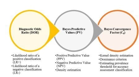
3.2. Bayesian Diagnostic and Predictive Metrics

3.2.1. Diagnostic Odds Ratio (DOR)

Using the definitions of sensitivity and specificity in the previous session, we can compute the likelihood ratio metric [60,61]. In a binary (Boolean) classification scheme, there are two forms of likelihood ratios: the likelihood ratio of a positive classification (LR+), and the likelihood ratio of a positive classification (LR-). The likelihood ratios are connected with levels of sensitivity and specificity directly [62] as such:
Entropy 15 02480 i007
The likelihood ratios obtained for a binary classification can be used to compute the value of an index for diagnostic inference, namely, the diagnostic odds ratio (DOR) index. The DOR represents simply the ratio of the positive to the negative likelihoods:
Entropy 15 02480 i008
The DOR can be interpreted as an unrestricted measure of the classification accuracy [62], but suffers from serious limitations, since both LR+ and LR- are sensitive to the threshold value (cut-off point) of the classification [63]. Thus, DOR can be used as a measure of the classification accuracy in cases where, (a) the threshold value of the binary classification is somewhat balanced (around 0.5), or; (b) when comparing classification schemes that have the same threshold value (e.g., in the case of simulation runs that are unbalanced but face similar threshold values).

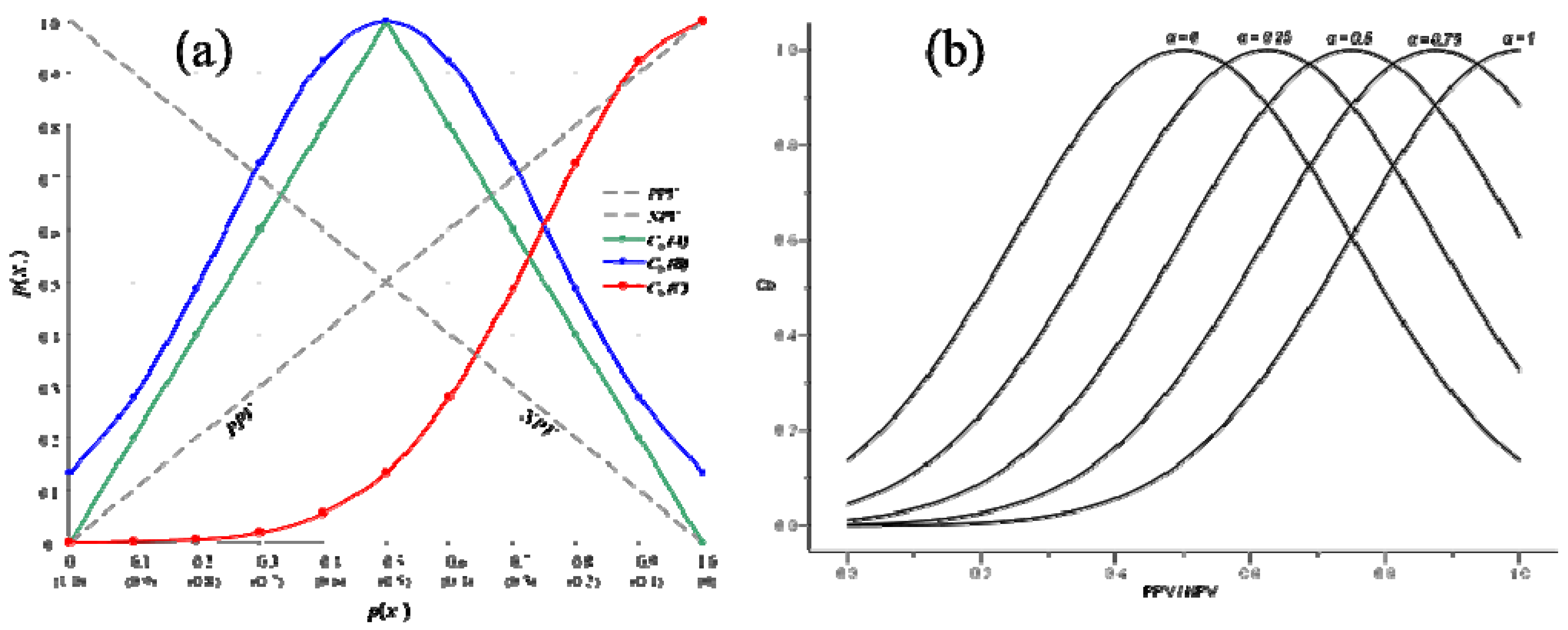
3.2.2. Bayesian Predictive Values for Positive and Negative Classification (PPV/NPV)

In place of the simple and practically limited DOR index to assess the robust spatial model accuracy, a Bayesian framework of assessment can be used. It uses the likelihood ratios (LR+ and LR−) to estimate a posterior probability classification based on the information embedded in the dataset. Strictly speaking, the model accuracy obtained by the confusion matrix (and consequently the sensitivity and specificity values), represents a prior probabilistic assessment of the model’s accuracy. This assessment is subject to the threshold value of the classification scheme. Obtaining a classification scheme that is robust enough to allow us to estimate model accuracy for a range of thresholds requires the computation of the conditional estimates [64]. This represents a posterior probabilistic assessment of the model’s accuracy, which can be achieved using Bayes’ Theorem. Computing the posterior Bayes probabilities for a positive and negative classification can be achieved using a general equation form:
Entropy 15 02480 i009
and:
Entropy 15 02480 i010
where:
PPV: the Bayes predictive value of a positive classification metric;
NPV: the Bayes predictive value of a negative classification metric;
x+,x-: the positive and negative values of the classification, and;
c: the prevalence threshold for which a value is positive if it is larger or equal from (computed using a ML nonparametric estimation).
The PPV and NPV values can be computed from the sensitivity and specificity values (and thus from the confusion matrix) as follows:
Entropy 15 02480 i011
and:
Entropy 15 02480 i012
In reality, the nature of the relationship between Bayesian predictive values and prevalence is likely to be nonmonotonic and can be defined by the posterior Bayesian estimator properties, namely the posterior density estimation [60,65].
To understand the role of the posterior Bayesian estimation, a theoretical problem formulation is provided in Figure 4. Part (a) of the figure provides a hypothetical prior density estimation of a binary classification scheme across a continuous range of classification thresholds (prevalence). For a given transitional change (e.g., presence of land use change), the prevalence threshold ranges from zero (purely negative) to one (purely positive). The left density curve represents the absence of a transition (negative classification), while the right density curve represents the presence of a transition (positive classification). As explained in the first section, when we lack any additional information about the classification threshold, the best uncertain choice (maximum entropy classification) is to assume an equal probability between the two classes (present, absent). In most of the cases involving spatial accuracy assessment, an uncertain prior is the best choice. Unlike the ROC curve method, where accuracy is assessed using a nonparametric estimation (without the use of a distribution function), the Bayesian estimation is based in a parametric assessment of the classification accuracy (or, at least a semiparametric assessment). In such an uncertain classification, we can vary only the spread of the distribution (i.e., the width of the density distribution) for each of the classes, but not the location of the threshold. As a consequence, the amount and proportions of the false negative (FN) and false positive (FP) allocations are affected only by the difference of the mean value of each of the transitions to the threshold. The more this difference is positive, the more likely it is for the transition to be present, while the more the difference is negative, the more likely it is for the transition to be absent.
Figure 4. Properties of the Bayesian estimation in binary classification scheme: (a) prior density estimation; (b) posterior density estimation, negative prevalence; (c) posterior density estimation, positive prevalence
Entropy 15 02480 g004
Thus, a posterior density Bayesian estimation allows us to estimate the probability densities of the classifications by adjusting the “true” height and “true” width of the density distributions.
We can perform a nonparametric estimation of the probability density function in the data by using a kernel density estimator such as the Epanechnikov stochastic kernel estimation [66]. The general equation of the kernel density function is [67,68]:
Entropy 15 02480 i013
where:
fk : an unknown continuous probability density function;
h: a smoothing parameter;
K(z): a symmetric kernel function, and;
N: the total number of independent observations of a random sample XN.
The equation for the Epanechnikov kernel density function is [67]:
Entropy 15 02480 i014
The choice of the Epanechnikov kernel density estimator is based on the high efficiency of this form in minimizing the asymptotic mean integrated square errors, AMISE [69,70], and it is often used in Neural Network computational learning [71]. While other estimators can be used to perform such kernel density estimation, the Epanechnikov estimator represents the most widely used and simpler form of the family of estimators.

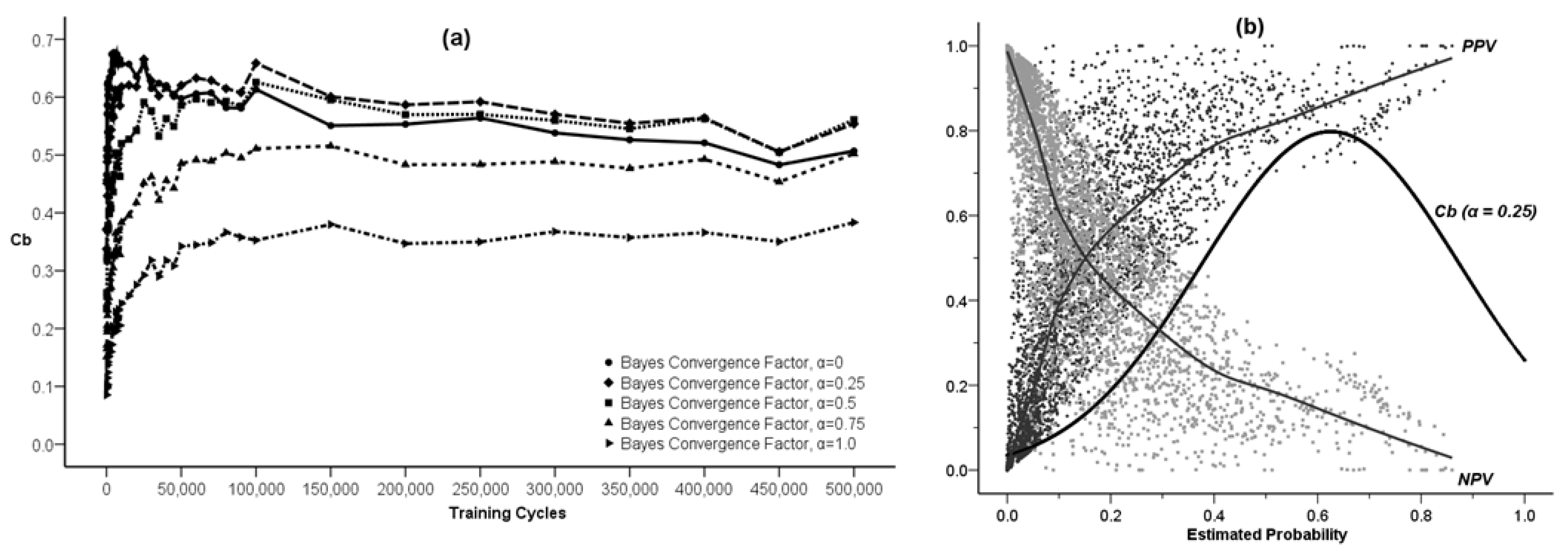
3.2.3. Bayesian Convergence Factor (Cb)

It is possible to derive an alternative accuracy metric that combines the two Bayesian predictive values, PPV and NPV, into a single, unified coefficient. The use of such a coefficient to measure classification and model accuracy is that it allows us to estimate not only a unique prevalence threshold, but also an optimal prevalence region for which our estimated accuracy is high for both positive and negative classifications. The analysis provided in the previous paragraph in the case of PPV and NPV metrics depends mainly on the choice of the kernel density estimation function and the continuous interval bandwidth used [67,72], or any other probability density function used for estimation. A unified Bayesian coefficient that measures the level of convergence between positive and negative predictive values permits us to derive a more robust prevalence region that smoothes the effect of density estimation selection. In other words, it provides us with a more global measure of model and classification assessment.
We have chosen to call this coefficient the Bayes convergence factor, Cb. A simple form of the factor can be defined as:
Entropy 15 02480 i015
A higher level of the Bayes convergence factor thus denotes a higher probability of convergence between a positive and a negative predictive value or probabilities of change. Because of the probability properties of such a coefficient, and the fact that always PPV + NPC ≤ 1 (the probability of change cannot exceed 1.0), the range of the Cb coefficient will be: 0 ≤ Cb ≤ 1.0. This simple form of the Bayes convergence factor is shown in the theoretical curve Cb (A) of Figure 5a. We can see that the allocation of the positive and negative classification probabilities in the Cb function represents a form of a triangular density function with minimum value of zero, maximum value of 1.0, and mean value of 0.5. A triangular density function provides a minimal amount of information about the relationship, configuration and pattern between the positive and negative predictive values in a model. As shown in Figure 5a, these predictive values by themselves may be better represented by non-linear relationships (e.g., kernel density estimators). Thus, a better convergence factor can be found that reflects a degree of nonlinearity in the modeling classification assessment.
Figure 5. (a) Theoretical distribution density functions for the Bayes convergence metric (Cb): (A) triangular; (B) adjusted normal; and (C) asymmetric normal. (b) Variations of the asymmetry parameter, α, in the expected normal form of the Bayes convergence factor.
Entropy 15 02480 g005
An alternative form of the Bayes convergence factor can be symbolically calculated using a normal density distribution function, adjusted to a continuous scale between 0 and 1.0. The equation of the Normal density function is:
Entropy 15 02480 i016
For a normal distribution with x = 0 and σ = 0.5, we can model the behavior of the mean value, by setting:
Entropy 15 02480 i017
and thus:
Entropy 15 02480 i018
We can also adjust for the coefficient scale (0 to 1.0) by multiplying the previous equation by a normalization factor:
Entropy 15 02480 i019
The adjusted normal form of the Bayes convergence factor, can expressed as:
Entropy 15 02480 i020
The adjusted normal density distribution function of the Cb coefficient can be seen as the curve Cb (B) of Figure 5(a), and in our data can be estimated by a Normal or Epanechnikov kernel density function.
The previous two forms of the Cb metric assume implicitly that the combined effect of the positive and negative classification processes in our model is symmetric toward achieving a better model (and classification) accuracy. It is appropriate for modeling landscape transformations where the presence of a transition implies the absence of a negative transition. In many spatial modeling processes, simulating binary change with such an implicit assumption cannot be made easily. For example, a model (such as LTM) that simulates land use change is parameterized and learns to recognize patterns on drivers of change related to a positive land use transition effect only. Model training and testing based on drivers of the transitional presence does not necessarily convey information on the probability of the absence of such a transition, as it is likely that other or additional drivers of the absence of the transition may be in effect over an ensemble of landscapes. Consequently, we can derive a better form of the Bayes conversion function by assuming a biased or asymmetric join distribution among the predictive values of positive and negative classification. Such an asymmetry would favor more positive than negative classifications, assuming that the model learns more about the transitional patterns from a combination of a high positive and low negative predictive value, rather than from a high negative and low positive predictive value (since the sum of the predictive values equals 1). The latter is especially important in estimating empirical distributions derived from unbiased real-world data, which is clearly in the SEWI case study. The amount of area that undertakes urban land use transition in the data is considerably less than the amount of area that observes an absence of such transition, and implementing an asymmetric Bayesian prior distribution would assign more weight in the positive (presence of transition) than in the negative (absence of transition) land areas.
We can formulate such an unequal conversion function by modifying the mean central tendency of the previous form, Cb (B). In other words, by simulating a different mean for the adjusted normal distribution function. We can call this form, adjusted asymmetric normal density distribution, and for the same numerical parameters, x = 0, and σ = 0.5, we can simulate the behavior of the mean value:
Entropy 15 02480 i021
where, α is the degree of asymmetry of our distribution (0 ≤ α ≤ 1). In other words, the parameter α denotes the degree of bias in terms of a theoretical least-cost function, or the relative informational balance in our model from a positive to negative predictive value.
The new asymmetric normal distribution will be:
Entropy 15 02480 i022
and, after adjusting for scale normalization, the final Bayes convergence factor will be:
Entropy 15 02480 i023
For varying levels of the parameter α, the shape of the latter convergence factor is shown in Figure 5b. For α = 0, the equation yields the symmetric normal form of the convergence factor (i.e., shape Cb (B) in Figure 5a), while, for α = 1, the equation yields a full asymmetric normal form of the convergence factor [i.e., shape Cb (C) in Figure 5(a)]. In an experimental dataset, any form of asymmetric normal distribution form of Cb (i.e., for any parameter α) can be estimated by a Normal of Epanechnikov kernel distribution function.

4. Results and Discussion

In the case of the SEWI region simulation runs, the computed DOR can be used to compare classification performance across training cycles (same areas, and same classification thresholds), but not across area groups or different simulation boxes. The results shown in Figure 6a signify the importance of pattern learning (training) process of improving the classification accuracy in the SEWI region experimental simulations.
The results for the PPV and NPV metrics obtained for the SEWI region and the three simulation area groups are shown in Figure 6b,c. Simulation area group C has consistently the higher PPV and the lowest NPV throughout the training exercise, a fact that signifies a higher model performance level than the ones achieved by simulation area groups A and B.
Figure 6. (a) Diagnostic Odds Ratio (DOR) index across LTM training cycles in the SEWI region. (b) Bayes probability of change given a positive classification (PPV). (c) Bayes probability of change given a negative classification (NPV) metric results by simulation group in the SEWI region
Entropy 15 02480 g006
Measuring and treating PPV and NPV as separate metrics of model performance is a rather trivial operation, and it is not a very useful or informative tool in assessing spatial model accuracy. However, by combining the PPV and NPV metrics into a single graph, we can illustrate the dominance relationships and dynamics over an expected prevalence threshold value (i.e., prevalence = 0.5, denoting an uninformative prior for the Bayesian classification). Figure 7 shows the dominance relationships between PPV and NPV for increasing LTM training cycles.
Figure 7. Dominance relations between Bayes PPV and NPV metrics: (a) area group A; (b) area group B; (c) area group C.
Entropy 15 02480 g007
In the simulation area group A, the model accuracy is based mainly on the dominant negative classification (although this dominance fades over the training process). The accuracy in simulation area group B is based on an unstable equilibrium between positive and negative classification (especially between 20,000 and 250,000 training cycles), although the overall accuracy is still supported by a dominant negative classification scheme. The model accuracy in simulation area C depends on a more desirable classification scheme, since after the first 10,000 cycles model accuracy depends consistently on a positive classification.
The analysis of the latter results is based on an expected, i.e., balanced prevalence threshold. As explained in the methodology section above, the relationship between Bayesian predictive values and prevalence is likely non-linear and a posterior Bayesian density estimator can be used to define this relationship more precisely.
The Bayesian estimation adjustment of the “true” values of the height and width of the SEWI empirically obtained distributions is shown in Figure 4 of the previous session. In Figure 4b, the changes in the density distributions for the threshold classes shifts the threshold prevalence value disproportional to the size and spread of each of the distributions. The posterior Bayesian density estimates allow us to evaluate the mean and variance of a new, “informative” prevalence threshold (shown with dotted line and shaded areas in Figure 4b).
The empirically obtained relationship between prevalence and the level of the PPV/NPV is shown in Figure 8. The y-axis of the graph represents the prevalence level (classification threshold), while the x-axis represents the level of the predictive value (PPV or NPV). The points that belong to the PPV and NPV are color-coded. The data points correspond to all sampled simulation runs (44 sampled training cycles for each of the 90 boxes in groups A, B and C, a total of 3,960 simulation run results).
The solid lines in Figure 8 represent the results of the Epanechnikov stochastic kernel estimation as methodologically described in the previous session.
In the SEWI region data, the underlying question that the analysis attempts to address is for which prevalence threshold value the “true” predictive value (and accuracy) of the modeled transitional classification becomes equal to the “true” absence of such transaction? Graphically, the solution can be found by varying the height of the y-axis reference line (horizontal dotted lines in Figure 8) over a fixed level of predictive value, where PPV = NPV = 0.5 (vertical dotted line). The y-axis coordinate for which the two kernel density estimated lines meet represents the prevalence threshold that maximizes the posterior probability of our model accuracy predictions. The behavior of other estimators beyond the Epanechnikov model have not been explored in this study, and represents a research question for future analysis and investigation.
Mathematically, the optimal prevalence threshold of the posterior probability distribution exists where:
Entropy 15 02480 i024
The difference between the prior and posterior estimation is shown in the vertical distance between the y-axis reference lines at the 0.5 prevalence threshold and the one at the meeting point of the two kernel density functions (~0.172 in the entire SEWI regions’ simulation data). The posterior estimation allows us to threshold at a lower classification level, thus enhancing the accuracy of our predictions.
Figure 8. Relationship between prevalence (y-axis) and the Bayes predictive values, PPV and NPV (x-axis). The solid lines represent the Epanechnikov kernel density estimation for PPV and NPV. The dotted reference lines identify the coordinates of the difference between expected and predicted prevalence thresholds. The colored solid reference lines indicate a graphically derived uncertainty bounding threshold.
Entropy 15 02480 g008
The results of the empirical data obtained for the SEWI region simulation runs for the varying degree of asymmetry in estimating the Bayes Convergence Factor, Cb, are shown in Figure 9a.
Figure 9. (a) Estimated mean Bayes convergence factor for varying levels of the asymmetry coefficient in the SEWI region; (b) Estimated probabilities of transition from the empirical values of the Bayes convergence factor (α = 0.25). Data points represent the estimated PPV and NPV values in the SEWI region (for all simulation boxes’ sampled training cycles).
Entropy 15 02480 g009
We can see that a somewhat moderate level of asymmetry (α = 0.25) performs consistently better throughout the entire model learning process (i.e., training cycles) despite the fact that at the 500,000 cycles training cycle level, the Bayes Convergence Factor with α = 0.5 performs slightly better. Thus, there is evidence in the SEWI simulation runs that a level of asymmetry in the composition of positive and negative predictive value of our model exists and thus should be incorporated into our spatial accuracy assessment.
Beyond any visual inspection and inference of our results, it is possible to derive quantitative estimates of the dominance of a level of asymmetry present in our simulation runs. As can be seen in Figure 9b we can estimate the expected probabilities of transitions, subject to the observed empirical values of transitions present in our simulation data. When all the simulation results for the entire SEWI region are examined with respect to their observed predictive values, we can estimate such an empirical probability distribution as a function of an estimated “true” mean (location parameter) and standard deviation (scale parameter) of each of the forms of Bayes Convergence Factor, Entropy 15 02480 i026 
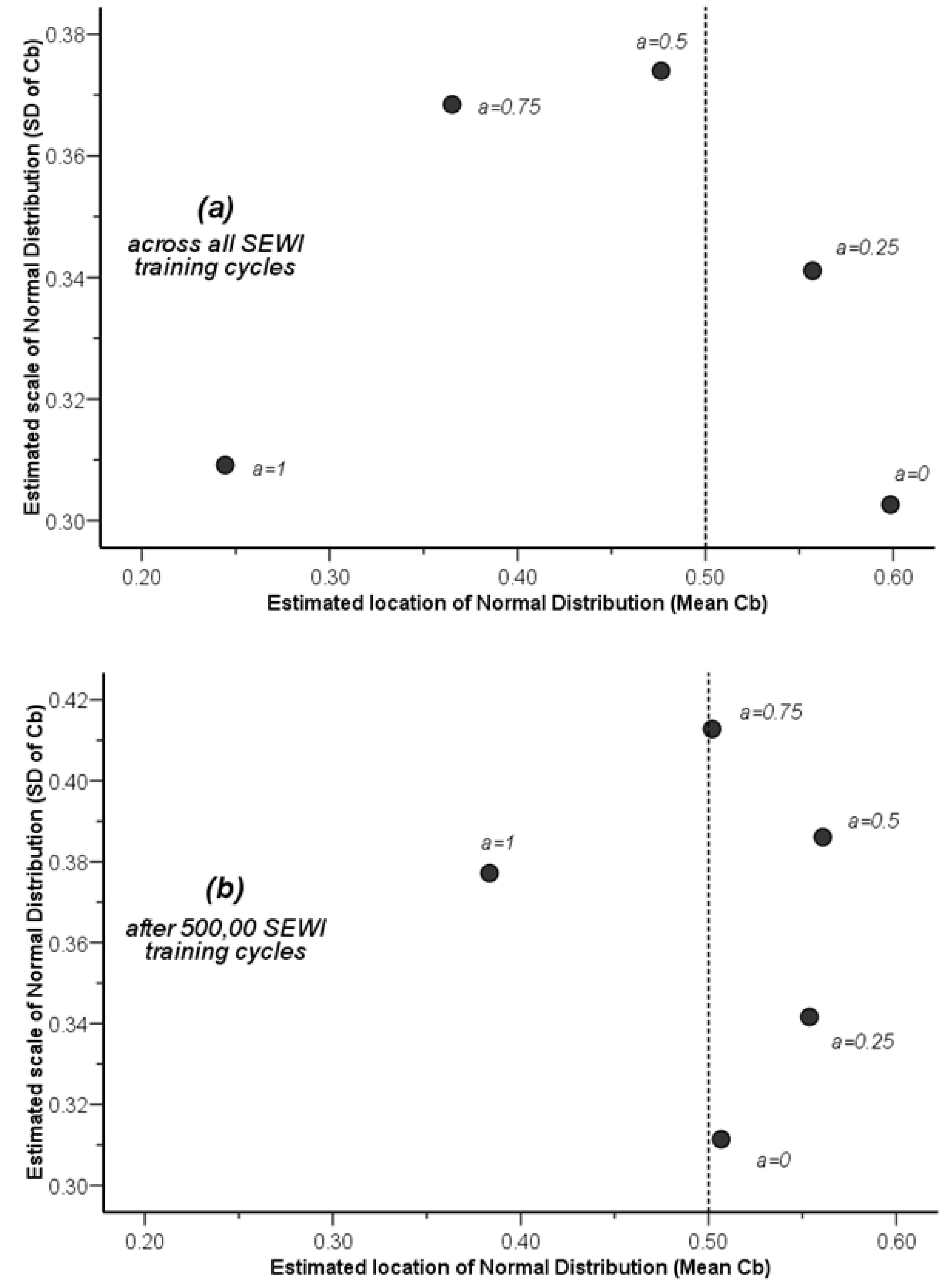
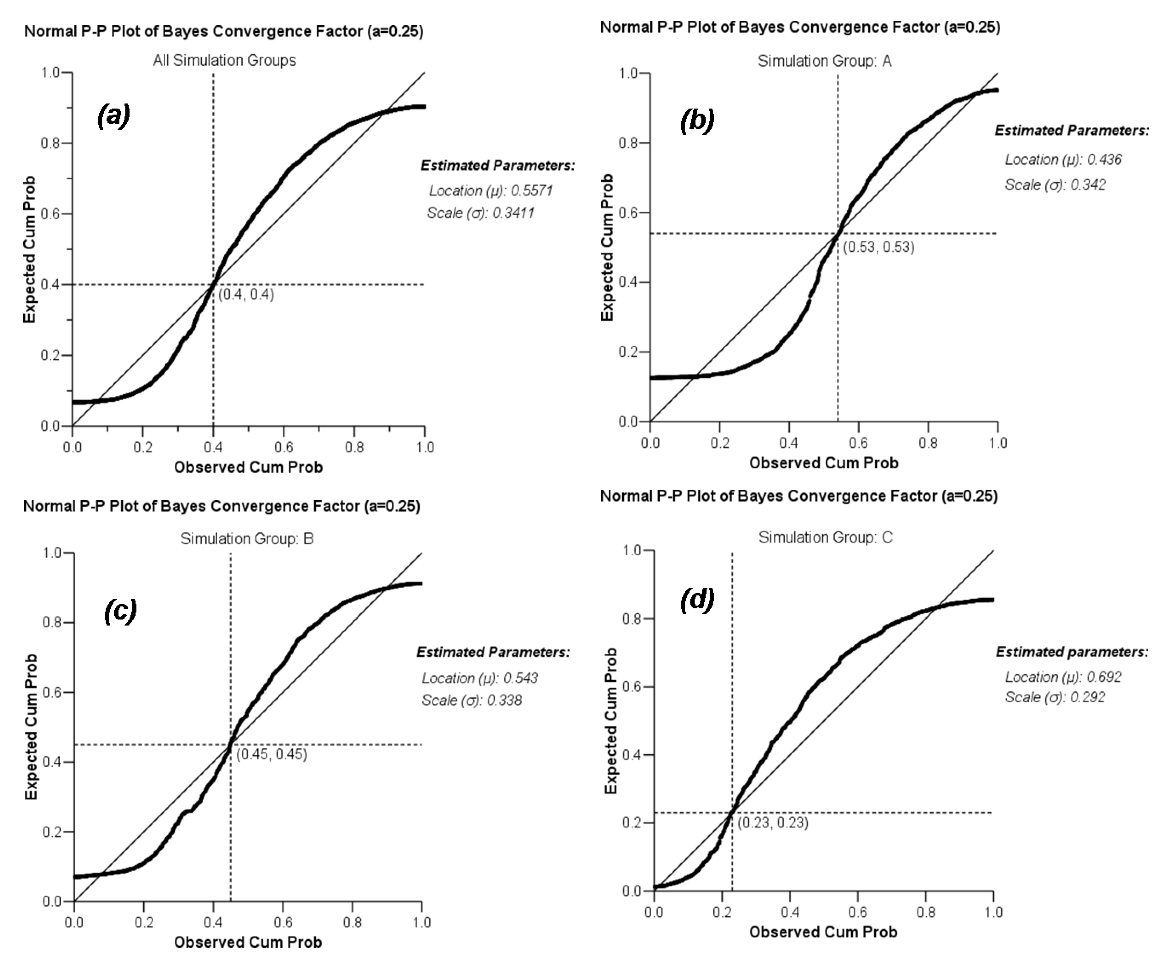
using a maximum likelihood estimation (ML) method. The results of such an estimation for the varying degree of asymmetry in the Bayes convergence factor in the SEWI data are shown in Table 2. Two groups of parameter estimates are included in the analysis: (a) parameter estimates across all SEWI simulation training cycles, indicating a robust model performance; (b) parameter estimates only after 500,000 training cycles in the SEWI simulation runs, indicating a model performance with emphasis on maximizing the information flows in modeling transformations in our landscape.
Table 2. Estimated values for the location (μ) and scale (σ) parameters of the empirical asymmetric Bayes Convergence Factor in the SEWI area
LevelPredicted Values for Bayes Convergence Factor
Selection LevelBayes Conversion Factor AsymmetryEstimated location of Normal Distribution (μ)Estimated scale of Normal Distribution (σ)
Across all training cyclesα = 0.00.59850.3027
α = 0.250.55710.3411
α = 0.50.47640.3740
α = 0.750.36510.3685
α = 1.00.24430.3092
After 500,000 training cyclesα = 0.00.50670.3114
α = 0.250.55370.3416
α = 0.50.56080.3861
α = 0.750.50190.4128
α = 1.00.38340.3772
Figure 10 plots the empirically obtained estimated parameters for location (x-axis) against scale (y-axis). Such a plot can help us select the best asymptotic form of the Bayes convergence factor using a dominance criterion, such as the mean-variance-robustness criterion. A desired probability distribution would have an estimated mean value closer to the 0.5 probability threshold (prevalence). Thus, estimated location parameters closer to 0.5 are dominant. On the other hand, we want our predicted probability distributions to minimize the level of uncertainty in our predictions. Thus, the estimated scale parameters with smaller values are dominant. Finally, a desired probability distribution would have relatively consistent estimated values of the location and scale parameters in both robust and informational assessments. We can see from Figure 9 that the only asymmetric form of the Bayes convergence factor that meets all three dominance criteria is the one with α = 0.25.
Figure 10. Estimated location (μ) and scale (σ) parameters of selected asymmetric normal forms of the Bayes convergence factor from empirical data in the SEWI region: (a) robust estimates (across all training cycles); (b) maximum information estimates (after 500,000 cycles)
Entropy 15 02480 g010
We can further enhance the quantitative assessment of the dominant asymmetric form of the Cb metric, by computing explicitly the dominance criteria. The three dominance criteria can be combined as:
Entropy 15 02480 i025
where, the symbol “≻” denotes dominant relationships, and:
i,j: unique combinations of location and scale (i.e., asymmetric forms of the Cb metric);
m,k: unique groups for testing robustness (i.e., training cycle groupings);
Entropy 15 02480 i027: mean (location) criterion;
Entropy 15 02480 i028: variance (scale) criterion;
Entropy 15 02480 i029: robustness criterion, and δ: any value or classification rule.
The results of the dominance criteria in the SEWI results visualized in Figure 10 are summarized in Table 3. The values of the table cells represent the values of the differences in Equation (25). The shaded cells signify the dominant asymmetric form of the Bayes convergence factor to be chosen.
Table 3. Dominance values for assessing the selection of the Cb asymmetric normal form in the SEWI region
Mean-Variance Groups Robustness Groups
All training cycles500,000 training cycles
α = 0.01.0710.071
α = 0.2516.74415.744
α = 0.50.286−0.714
α = 0.750.987−0.013
α = 1.01.5960.596
Selecting the appropriate asymmetric form of the Bayes convergence factor allows us to infer additional information about the overall performance of our model. We can measure the deviation from a symmetric normal distribution (expected prior probabilities) that the estimated asymmetric form of the Bayesian convergence factor (observed posterior probabilities) yields. The P-P plots of this assessment are shown in Figure 11. The thick curve represents the estimated cumulative probability distribution of the asymmetric Cb predictive values observed in the SEWI region, estimated from the simulation data. The estimated parameters (location, scale) are shown in the right side of each graph. The diagonal line represents the expected cumulative probability distribution of a symmetric distribution of predictive values (i.e., the expected predictive values at a prevalence threshold of 0.5). The parts of the predicted cumulative distribution curve that are above the expected one (diagonal) signifies an increase in model accuracy that can be obtained from an asymmetric classification, while the parts of the predictive cumulative distribution curve below the expected diagonal line, signifies a decrease in model accuracy. The point where the two lines meet (shown as the point of intersection of the reference lines), provide us with an estimated empirical prevalence level (threshold value for classification) that maximizes the simulated accuracy in our data. The net gain (or loss) in predictive value of our model due to the uncertainty in classification is the difference in the area that rests between the expected diagonal line and the estimated observed curve, after determining the optimal (dominant) choice of the asymmetric form parameters of the Bayes convergence factor.
Figure 11. Normal P-P plots for assessing Bayesian convergence simulation performance of the SEWI region: (a) across all simulation groups; (b) simulation group A; (c) simulation group B; (d) simulation group C.
Entropy 15 02480 g011
From an initial observation of the models’ accuracy within all simulation runs in the SEWI region, shown in sub-graph (a) of Figure 11, the estimated prevalence threshold (= 0.4) does not seem to deviate importantly from the expected one (0.5). Shifting the prevalence threshold would provide a 5.7% increase in the predictive value (informational gain) of the model. But, if we repeat our analysis for the SEWI regions’ simulation groups (A, B and C), thus accounting for structural differences in the proportion of urban cells and exclusionary areas, we can see that spatial configuration affects considerably our actual model performance. For simulation group A, shown in sub-graph (b), the model performance is heavily dependent on the negative predictive values (estimated prevalence of 0.53 > 0.5), and produces poor overall model predictive values (Cb = 0.436, or a 6.4% decrease in mean predictive value of the model). As the proportion of urban to exclusionary increases in the spatial composition of our simulation maps, the predictive value of the model increases substantially, and the estimated prevalence level decreases. Especially for group C, shown in sub-graph (d), a gain of 19.2% in model performance can be obtained from a shift in model prevalence (from 0.5 to 0.23).

5. Conclusions

The analysis described above reveals the magnitude and multi-dimensionality of the spatial complexity involved in modeling landscape transformations in mixed and asymmetric landscapes in terms of amount and distribution of change. Performing spatial accuracy assessment requires the development and utilization of additional, advanced methods of assessment, related both to the models’ predictive value in terms of quantity of change, but also to the performance of classifying the presence or absence of such a transition. It has been shown above that classification accuracy is closely related to the achieved modeling performance, and additional Bayesian metrics have been proposed, described and analyzed using the SEWI region case study. These advanced methods take into advantage the stochastic character of complex simulation models such as the LTM model, and can be used for performing model assessment in many other land change models that use intelligence-based tools, such as agent-based models of land use change, or other spatially explicit artificial intelligent modeling like cellular automata and genetic algorithms. The metrics described in this paper address different aspects of the spatial modeling performance such as assessing the predictive value of the model simulations (PPV, NPV, DOR) and estimating empirical convergence curves for enhancing classification accuracy (Cb). The proposed metrics, and their assessment methodology, allows the researcher and analyst to acquire a more holistic assessment of a models’ spatial accuracy over space and time, especially in the presence of uncertainty about the transitional model thresholds.
The case study of the SEWI region used to illustrate the usage of the metrics, allow us to assess the LTM model accuracy for simulating urban changes in the region. All metrics confirm a general emergent model accuracy converging towards a 70% upper level for the data analyzed and presented in this study (i.e., in the SEWI area urban transitions). We can also see how the amount of urban change and exclusionary zones present in our landscapes dramatically affects the performance of the model. The latter result raises the significance of adjusting the classification prevalence threshold at spatially homogeneous scales in our simulation groups (e.g., implementing different thresholds for groups with different classes of urban change).
The results obtained also allow us to infer that in landscapes where the rate and amount of land use change varies substantially, symmetric spatial transition classification schemes are difficult to obtain. Instead we can enhance model predictions by assuming asymmetric spatial configurations, and by estimating the degree of asymmetry via a spatial stochastic dominance methodology. The practical significance of the proposed additional spatial model assessment metrics is that they can provide an “informational summary” of the simulated region or landscape ensembles. The use of the analysis and the performance of the metrics can help us in a multitude of ways. First, to understand and learn how well the model fits to different combinations of presence and absence of transitions in our landscapes, not simply how well the model fits our given data. Second, given that most spatial databases suffer from incomplete information and pre-simulation measurement errors, we can also derive (estimate) a theoretical accuracy that we would expect our model to assess, under the presence of such incomplete information data, and thus partially separate model from measurement errors in spatial simulations. Third, to understand the role and pattern of uncertainty in our simulations and model estimations. We can compare results across simulation runs (and thus quantitative patterns of change) that tend to provide less or more uncertain model performance, and understand the role of spatially-explicit patterns and cell configurations to model training and simulation. Fourth, to compare the significance or estimation contribution of transitional presence and absence (change versus no change) to our model performance, and the contribution of the spatial drivers and variables to the explanatory value of our model. Estimating model performance using different combinations of drivers (e.g., instead of groups A, B, C in the SEWI region, use of the same sampled boxes with different drivers, or using training sets with sequentially dropping a driver at a time), could allow us to estimate the differences in informational uncertainty for each driver combination or for single drivers within our simulations. Fifth, to compare measurements of informational uncertainty at different scales of spatial resolution. Pijanowski et al. [13,57] showed the significance of using a scalable window for sensitivity analysis. Assessing model uncertainty of predictions for each of spatial resolutions can also enhance our knowledge about modeling at different spatial scales and selecting scales that produce lower uncertainty estimates.
The methodology and metrics developed in this paper allow for the development of a more comprehensive dynamic and adaptive modeling methodology. Beyond the aggregate level for which the assessment was performed for the purposes of this paper, it is both methodologically and computationally feasible to assess and adjust model accuracy at a simulation-to-simulation basis, in order to obtain dynamically enhanced simulation results. Especially in the case of agent-based modeling such a model assessment methodology can be inversed and iterated to obtain spatially robust and diverse future landscape configurations that optimize both the amount and degree of information contained in the simulation, and the emergence of stochastically dominant agent strategies.
Finally, in terms of the “real-world” significance to the community of land use planning practitioners, the analyses presented in this paper can be used to highlight a number of issues regarding modeling urban transitions, specifically: (a) simple, traditional modeling techniques are not adequate to accurately capture the uncertainty present as a direct result of the rarity of the urban/suburban changes (e.g., when only small amount of changes are expected or predicted to emerge); (b) accuracy assessment and validation modeling properties are very important, especially when comparing different models or different areas with varying quantities and characteristics of urban change transitions, and; (c) a greater awareness by practitioners of more advanced and stochastic modeling techniques can potentially increase the effectiveness of planning efforts.

Acknowledgments

Partial funding for the research was provided by the Great Lakes Fishery Trust and the US EPA STAR Program. Additional funding was provided by the National Science Foundation’s Virgin Islands Experimental Program to Stimulate Competitive Research, VI-EPSCoR (award no. 0814417). The author’s wish to thank the planners and the Southeastern Wisconsin Regional Planning Commission for the provision of the original data used in this analysis, as well as Dr. Daniel Muller for the input and comments during the modeling and analysis stages of this study.

Conflict of Interest

The authors declare no conflict of interest.

References

  1. Lambin, E.F.; Geist, H. Land-Use and Land-Cover Change: Local Processes and Global Impacts; Springer-Verlag: Berlin, Germany, 2006. [Google Scholar]
  2. Pijanowski, B.C.; Robinson, K.D. Rates and patterns of land use change in the upper Great Lakes States, USA: A framework for spatial temporal analysis. Landscape Urban Plan. 2011, 102, 102–116. [Google Scholar] [CrossRef]
  3. Committee on grand challenges in environmental sciences, oversight commission for the committee on grand challenges in environmental sciences. Grand Challenges in Environmental Sciences; The National Academies Press: Washington, D.C., USA, 2001. [Google Scholar]
  4. Ray, D.K.; Pijanowksi, B.C.; Kendall, A.D.; Hyndman, D.W. Coupling land use and groundwater models to map land use legacies: Assessment of model uncertainties relevant to land use planning. Appl. Geogr. 2012, 34, 356–370. [Google Scholar] [CrossRef]
  5. Pijanowski, B.C.; Ray, D.K.; Kendall, A.D.; Duckles, J.M.; Hyndman, D.W. Using backcast land-use change and groundwater travel-time models to generate land-use legacy maps for watershed management. Ecol. Soc. 2007, 12, 25:1–25:19. [Google Scholar]
  6. Yang, G.; Bowling, L.C.; Chherkauer, K.A.; Pijanowksi, B.C. The impact of urban development on hydrologic regime from catchment to basin scales. Landscape Urban Plan. 2011, 103, 237–247. [Google Scholar] [CrossRef]
  7. Mishra, V.; Cherkauer, K.A.; Niyogi, D.; Lei, M.; Pijanowski, B.C.; Ray, D.K.; Bowling, L.C.; Yang, G. A regional scale assessment of land use/land cover and climatic changes on water and energy cycle in the upper Midwest United States. Int. J. Climatol. 2010, 30, 2025–2044. [Google Scholar] [CrossRef]
  8. Pijanowski, B.; Moore, N.; Mauree, D.; Niyogi, D. Evaluating error propagation in coupled land-atmosphere models. Earth Interact. 2011, 15, 1–25. [Google Scholar] [CrossRef]
  9. Wiley, M.J.; et al. A multi-modeling approach to evaluating climate and land use change impacts in a Great Lakes River Basin. Hydrobiologia 2010, 657, 243–262. [Google Scholar]
  10. Wayland, K.G.; Hyndman, D.W.; Boutt, D.; Pijanowski, B.C.; Long, D.T. Modeling the impact of historical land uses on surface water quality using ground water flow and solute transport models. Lakes Reserv. Res. Manag. 2002, 7, 189–199. [Google Scholar] [CrossRef]
  11. Pontius, R.G., Jr.; Boersma, W.; Castella, J.-C.; Clarke, K.; Nijs, T.D.; Dietzel, C.; Duan, Z.; Fostsing, E.; Goldstein, N.; Kok, K.; et al. Comparing the input, output, and validation maps for several models of land change. Ann. Reg. Sci. 2008, 42, 11–37. [Google Scholar]
  12. Pontius, R.G., Jr.; Neeti, N. Uncertainty in the difference between maps of future land change scenarios. Sustain. Sci. 2010, 5, 39–50. [Google Scholar] [CrossRef]
  13. Pijanowski, B.C.; Pithadia, S.; Shellito, B.A.; Alexandridis, K. Calibrating a neural network-based urban change model for two metropolitan areas of the upper midwest of the United States. Int. J. Geogr. Inf. Sci. 2005, 19, 197–215. [Google Scholar] [CrossRef]
  14. Pijanowski, B.C.; Alexandridis, K.T.; Müller, D. Modelling urbanization patterns in two diverse regions of the world. J. Land Use Sci. 2006, 1, 83–108. [Google Scholar] [CrossRef]
  15. Pontius, R.G., Jr.; Millones, M. Death to Kappa: Birth of quantity disagreement and allocation disagreement for accuracy assessment. Int. J. Remote Sens. 2011, 32, 4407–4429. [Google Scholar] [CrossRef]
  16. Shannon, C.E. A mathematical theory of communication. Bell Syst. Tech. J. 1948, 27, 379–423, Reprinted with corrections: 623–656, 1948. [Google Scholar] [CrossRef]
  17. Shannon, C.E.; Weaver, W. Mathematical Theory of Communication; University of Illinois Press: Chicago, IL, USA, 1963. [Google Scholar]
  18. Jessop, A. Informed Assessments: An Introduction to Information, Entropy, and Statistics; Ellis Horwood: New York, NY, USA, 1995; p. 366. [Google Scholar]
  19. Vajda, I. Theory of Statistical Inference and Information; Kluwer Academic Publishers: Dordrecht, The Netherlands, 1989; p. 432. [Google Scholar]
  20. Stoica, P.; Selen, Y.; Li, J. Multi-model approach to model selection. Digit. Signal Process. 2004, 14, 399–412. [Google Scholar] [CrossRef]
  21. Nelson, T.; Boots, B.; Wulder, M.A. Techniques for accuracy assessment of tree locations extracted from remotely sensed imagery. J. Environ. Manag. 2005, 74, 265–271. [Google Scholar] [CrossRef] [PubMed]
  22. Roloff, G.J.; Haufler, J.B.; Scott, J.M.; Heglund, P.J.; Morrison, M.L.; Haufler, J.B.; Raphael, M.G.; Wall, W.A.; Samson, F.B. Modeling Habitat-based Viability from Organism to Population. In Predicting Species Occurences: Issues of Accuracy and Scale; Island Press: Washington, D.C., USA, 2002; pp. 673–686. [Google Scholar]
  23. James, F.C.; McGulloch, C.E.; Scott, J.M.; Heglund, P.J.; Morrison, M.L.; Haufler, J.B.; Raphael, M.G.; Wall, W.A.; Samson, F.B. Predicting Species Presence and Abundance. In Predicting Species Occurences: Issues of Accuracy and Scale; Island Press: Washington, D.C., USA, 2002; pp. 461–466. [Google Scholar]
  24. Gonzalez-Rebeles, C.; Thompson, B.C.; Bryant, F.C.; Scott, J.M.; Heglund, P.J.; Morrison, M.L.; Haufler, J.B.; Raphael, M.G.; Wall, W.A.; Samson, F.B. Influence of Selected Environmental Variables on GIS-Habitat Models Used for Gap Analysis. In Predicting Species Occurences: Issues of Accuracy and Scale; Island Press: Washington, D.C., USA, 2002; pp. 639–652. [Google Scholar]
  25. Lowell, K.; Jaton, A. Spatial Accuracy Assessment: Land Information Uncertainty in Natural Resources; Ann Arbor Press: Chelsea, MI, USA, 1999; p. 455. [Google Scholar]
  26. Cablk, M.; White, D.; Kiester, A.R.; Scott, J.M.; Heglund, P.J.; Morrison, M.L.; Haufler, J.B.; Raphael, M.G.; Wall, W.A.; Samson, F.B. Assessment of Spatial Autocorrelation in Empirical Models in Ecology. In Predicting Species Occurences: Issues of Accuracy and Scale; Island Press: Washington, D.C., USA, 2002; pp. 429–440. [Google Scholar]
  27. Wu, J.; Hobbs, R. Key issues and research priorities in landscape ecology: An idiosyncratic synthesis. Landscape Ecol. 2002, 17, 355–365. [Google Scholar] [CrossRef]
  28. McKenney, D.W.; Venier, L.A.; Heerdegen, A.; McCarthy, M.A.; Scott, J.M.; Heglund, P.J.; Morrison, M.L.; Haufler, J.B.; Raphael, M.G.; Wall, W.A.; et al. A Monte Carlo experiment for species mapping problems. In Predicting Species Occurences: Issues of Accuracy and Scale; Island Press: Washington, D.C., USA, 2002; pp. 377–382. [Google Scholar]
  29. Gelfand, A.E.; Schmidt, A.M.; Wu, S.; Silander, J.A.; Latimer, A.; Rebelo, A.G. Modelling species diversity through species level hierarchical modelling. J. R. Stat. Soc. Ser. C Appl. Stat. 2005, 54, 1–20. [Google Scholar] [CrossRef]
  30. Pontius, G.R., Jr.; Spencer, J. Uncertainty in extrapolations of predictive land-change models. Environ. Plan. B—Plan. Des. 2005, 32, 211–230. [Google Scholar]
  31. Sun, H.; Forsythe, W.; Waters, N. Modeling urban land use change and urban sprawl: Calgary, Alberta, Canada. Netw. Spat. Econ. 2007, 7, 353–376. [Google Scholar] [CrossRef]
  32. Berry, B.J.L.; Kiel, L.D.; Elliot, E. Adaptive agents, intelligence, and emergent human organization: Capturing complexity through agent-based modeling. Proc. Natl. Acad. Sci. U.S.A. 2002, 99, 7178–7188. [Google Scholar] [CrossRef] [PubMed]
  33. North, M.; Macal, C.; Campbell, P. Oh behave! Agent-based behavioral representations in problem solving environments. Future Gener. Comput. Syst. 2005, 21, 1192–1198. [Google Scholar]
  34. Alexandridis, K.T.; Pijanowski, B.C. Assessing multiagent parcelization performance in the mabel simulation model using monte carlo replication experiments. Environ. Plan. B—Plan. Des. 2007, 34, 223–244. [Google Scholar] [CrossRef]
  35. Brown, D.G.; Page, S.E.; Riolo, R.; Zellner, M.; Rand, W. Path dependence and the validation of agent-based spatial models of land use. Int. J. Geogr. Inf. Sci. 2005, 19, 153–174. [Google Scholar] [CrossRef]
  36. Fortin, M.J.; Boots, B.; Csillag, F.; Remmel, T.K. On the role of spatial stochastic models in understanding landscape indices in ecology. Oikos 2003, 102, 203–212. [Google Scholar] [CrossRef]
  37. Demetrius, L.; Matthias Gundlach, V.; Ochs, G. Complexity and demographic stability in population models. Theor. Popul. Biol. 2004, 65, 211–225. [Google Scholar] [CrossRef] [PubMed]
  38. Luijten, J.C. A systematic method for generating land use patterns using stochastic rules and basic landscape characteristics: Results for a Colombian hillside watershed. Agric. Ecosyst. Environ. 2003, 95, 427–441. [Google Scholar] [CrossRef]
  39. Boyen, X.; Koller, D. Approximate Learning of Dynamic Models. In Advances in Neural Information Processing Systems (NIPS 1998), Denver, Colorado, December 1998; MIT Press: Cambridge, MA, USA, 1999; pp. 396–402. [Google Scholar]
  40. Dubra, J.; Ok, E.A. A model of procedural decision making in the presence of risk. Int. Econ. Rev. 2002, 43, 1053–1080. [Google Scholar] [CrossRef]
  41. Lazrak, A.; Quenez, M.C. A generalized stochastic differential utility. Math. Oper. Res. 2003, 28, 154–180. [Google Scholar] [CrossRef]
  42. Fokoue, E.; Titterington, D.M. Mixtures of factor analysers, bayesian estimation and inference by stochastic simulation. Mach. Learn. 2003, 50, 73–94. [Google Scholar] [CrossRef]
  43. Kleijnen, J.P.C. An overview of the design and analysis of simulation experiments for sensitivity analysis. Eur. J. Oper. Res. 2005, 164, 287–300. [Google Scholar] [CrossRef]
  44. Aptekarev, A.I.; Dehesa, J.S.; Yanez, R.J. Spatial entropy of central potentials and strong asymptotics of orthogonal polynomials. J. Math. Phys. 1994, 35, 4423–4428. [Google Scholar] [CrossRef]
  45. Brink, A.D. Minimum spatial entropy threshold selection. IEEE Proc. Vis. Image Signal Process. 1995, 142, 128–132. [Google Scholar] [CrossRef]
  46. Batten, D.F. Complex landscapes of spatial interaction. Ann. Reg. Sci. 2001, 35, 81–111. [Google Scholar] [CrossRef]
  47. Chen, K.; Irwin, E.; Jayaprakash, C.; Warren, K. The emergence of racial segregation in an agent-based model of residential location: The role of competing preferences. Comput. Math. Organ. Theory 2005, 11, 333–338. [Google Scholar] [CrossRef]
  48. Yin, L.; Brian, M. Residential location and the biophysical environment: Exurban development agents in a heterogeneous landscape. Environ. Plan. B—Plan. Des. 2007, 34, 279–295. [Google Scholar] [CrossRef]
  49. Munroe, D.K. Exploring the determinants of spatial pattern in residential land markets: amenities and disamenities in Charlotte, NC, USA. Environ. Plan. B—Plan. Des. 2007, 34, 336–354. [Google Scholar] [CrossRef]
  50. Carrion-Flores, C.; Irwin, E.G. Determinants of residential land-use conversion and sprawl at the rural-urban fringe. Am. J. Agric. Econ. 2004, 86, 889–904. [Google Scholar] [CrossRef]
  51. Parker, D.C.; Meretsky, V. Measuring pattern outcomes in an agent-based model of edge-effect externalities using spatial metrics. Agric. Ecosyst. Environ. 2004, 101, 233–250. [Google Scholar] [CrossRef]
  52. Reginster, I.; Rounsevell, M. Scenarios of future urban land use in Europe. Environ. Plan. B—Plan. Des. 2006, 33, 619–636. [Google Scholar] [CrossRef]
  53. Veldkamp, A. Investigating land dynamics: Future research perspectives. J. Land Use Sci. 2009, 4, 5–14. [Google Scholar] [CrossRef]
  54. Pijanowski, B.C.; Shellito, B.; Pithadia, S.; Alexandridis, K. Forecasting and assessing the impact of urban sprawl in coastal watersheds along eastern Lake Michigan. Lakes Reser. Res. Manag. 2002, 7, 271–285. [Google Scholar] [CrossRef]
  55. Tayyebi, A.; Pekin, B.K.; Pijanowski, B.C.; Plourde, J.D.; Doucette, J.S.; Braun, D. Hierarchical modeling of urban growth across the conterminous USA: Developing meso-scale quantity drivers for the Land Transformation Model. J. Land Use Sci. 2012, 8, 1–21. [Google Scholar] [CrossRef]
  56. SEWRPC Digital Land Use Inventory; SouthEastern Wisconsin Regional Planning Commission (SEWRPC): Waukesha, WI, USA, 2000. Available http://maps.sewrpc.org/regionallandinfo/metadata/Land_Use_Inventory.htm (accessed on 24 June 2013).
  57. Pijanowski, B.C.; Brown, D.G.; Shellito, B.A.; Manik, G.A. Using neural networks and GIS to forecast land use changes: A land transformation model. Comput. Environ. Urban Syst. 2002, 26, 553–575. [Google Scholar] [CrossRef]
  58. Foody, G.M. Status of land cover classification accuracy assessment. Remote Sens. Environ. 2002, 80, 185–201. [Google Scholar] [CrossRef]
  59. Sousa, S.; Caeiro, S.; Painho, M. Assessment of map similarity of categorical maps using kappa statistics: The case of sado estuary. In Proceedings of ESIG 2002, Tagus Park, Oeiras, Portugal, 17–19 July 2002; Associacao de Utilizadores de Informacao Geografica: Tagus Park, Oeiras, Portugal, 2002. [Google Scholar]
  60. Brenner, H.; Gefeller, O. Variation of sensitivity, specificity, likelihood ratios and predictive values with disease prevalence. Stat. Med. 1997, 16, 981–991. [Google Scholar] [CrossRef]
  61. Suh, Y.T. Signal Detection in Noises of Unknown Powers Using Two-Input Receivers; University of Michigan: Ann Arbor, MI, USA, 1983; p. 153. [Google Scholar]
  62. Glas, A.S.; Lijmer, J.G.; Prins, M.H.; Bonsel, G.J.; Bossuyt, P.M.M. The diagnostic odds ratio: A single indicator of test performance. J. Clin. Epidemiol. 2003, 56, 1129–1135. [Google Scholar] [CrossRef]
  63. Pepe, M.S.; Janes, H.; Longton, G.; Leisenring, W.; Newcomb, P. Limitations of the odds ratio in gauging the performance of a diagnostic, prognostic, or screening marker. Am. J. Epidemiol. 2004, 159, 882–890. [Google Scholar] [CrossRef] [PubMed]
  64. Schafer, J.; Strimmer, K. An empirical Bayes approach to inferring large-scale gene association networks. Bioinformatics 2005, 21, 754–764. [Google Scholar] [CrossRef] [PubMed]
  65. Smith, J.E.; Winkler, R.L.; Fryback, D.G. The first positive: Computing positive predictive value at the extremes. Ann. Intern. Med. 2000, 132, 804–809. [Google Scholar] [CrossRef] [PubMed]
  66. Hart, J.D.; Wehrly, T.E. Kernel regression estimation using repeated measurements data. J. Am. Stat. Assoc. 1986, 81, 1080–1088. [Google Scholar] [CrossRef]
  67. Silverman, B.W. Density Estimation for Statistics and Data Analysis; CRC Press: London, UK, 1986; p. 175. [Google Scholar]
  68. Simonoff, J.S. Smoothing methods in statistics; Springer: New York, NY, USA, 1996; p. 338. [Google Scholar]
  69. Tapia, R.A.; Thompson, J.R. Nonparametric probability density estimation; Johns Hopkins University Press: Baltimore, MD, USA, 1978; p. 176. [Google Scholar]
  70. Wand, M.P.; Jones, M.C. Kernel Smoothing; Chapman & Hall: London, UK, 1995; p. 212. [Google Scholar]
  71. Smyth, P. Probability density estimation and local basis function neural networks. In Computational Learning Theory and Natural Learning Systems; Hanson, S.J., Petsche, T., Rivest, R.L., Kearns, M., Eds.; MIT Press: Cambridge, MA, USA, 1994; Volume II, pp. 233–248. [Google Scholar]
  72. Hansen, B.E. Sample splitting and threshold estimation. Econometrica 2000, 68, 575–603. [Google Scholar] [CrossRef]

