1. Introduction
Morphological computation is discussed in various contexts, such as DNA computing and self-assembly (see [
1,
2] for an overview). This work is concerned with morphological computation in the field of embodied intelligence. In this context it is often described as the trade-off between morphology and control [
3], which means that a well-chosen morphology can reduce the amount of required control substantially. Hereby, a morphology refers to the body of a system, explicitly including all its physiological and physical properties (shape, sensors, actuators, friction, mass distribution,
etc.) [
4]. The consensus is that morphological computation is the contribution of the morphology and environment to the behaviour that cannot be assigned to a nervous system or a controller. Theoretical work on describing morphological computation in this context has been conducted by [
5,
6].
The following quote very nicely describes how the shape of an insect wing in flight is not entirely determined by the muscular system, but by the interaction of the wings’ morphology with the environment:
However, active muscular forces cannot entirely control the wing shape in flight. They can only interact dynamically with the aerodynamic and inertial forces that the wings experience and with the wing’s own elasticity; the instantaneous results of these interactions are essentially determined by the architecture of the wing itself: its planform and relief, the distribution and local mechanical properties of the veins, the local thickness and properties of the membrane, the position and form of lines of flexion. The interpretation of these characters is the core of functional wing morphology.
The last sentence of this quote nicely summaries that the function of the wing is determined by the interaction of the environment with the physical properties of the wing. It is the quantification of this sort of contribution of the morphology to the behaviour of a system that is in the focus of this work. The difference to previous literature by Paul [
8] and Lundh [
9], who investigated morphological computational with respect to either the actuation (Paul) or the sensors (Lundh) only, is that we will measure morphological computation of embodied agents acting in the sensori-motor loop, including both sensors and actuators.
To understand which aspects a measure must cover and which it should omit, this paragraph will discuss two different artificial systems that show morphological computation. The most vivid example in this context is the Passive Dynamic Walker by McGeer [
10]. In this example, a two-legged walking machine preforms a naturally appealing walking behaviour, without any need of control, as a result of a well-chosen morphology and environment. There is simply no computation available, and the walking behaviour is the result of the gravity, the slope of the ground and the specifics of the mechanical construction (weight and length of the body parts, deviation of the joints,
etc.). If any parameter of the mechanics (morphology) or the slope (environment) is changed, the walking behaviour will not persist. Hence, we will only investigate morphological computation as an effect that emerges from the interaction of the control system, the body and the environment, also known as the sensori-motor loop (see next section). The Passive Dynamic Walker is, in this context, understood as an embodied agent without actuation. The behaviour of such a system is also discussed in the context of
natural dynamics [
11].
One may argue that the Passive Dynamic Walker is a purely mechanical system, and that speaking of morphological computation is an overstatement in this case. This is a valid point of view, as purely mechanical system does not perform calculations as we intuitively understand the term. Nevertheless, we claim that it is not an overstatement in the case of the Passive Dynamic Walker, as this system was explicitly built to simulate the morphological computation that is present in the human walking behaviour. For this purpose, a mechanical system was constructed that reflects the morphological properties of the lower half of a human body as far as it is required to understand and model the principles involved in human walking. Therefore, the Passive Dynamic Walker is allegoric for morphological computation present in the locomotion of humans.
A second impressive example for morphological computation is BigDog [
12]. This robot is a four-legged walking machine, which is built as a companion for humans operating in the field. The outstanding feature, with respect to this paper, is its morphological design. Instead of classical electric motors, BigDog has hydraulic actuators, which enable it to handle situations in which other walking machines would fail and even suffer severe damage. Most impressive is the video, which shows how BigDog handles a very slippery ground [
13]. Watching the video, it seems impossible to program such a balancing behaviour for an arbitrarily slippery ground. That BigDog is nevertheless able to cope with it is also the result of the hydraulic actuators and the well-chosen morphological design in general, which are both nicely documented in the video clip [
13].
The next step is to analyse what both examples have in common and in which aspects the two applications differ. The first obvious difference is the amount of available computation. Morphological computation is most often associated with low computational power that leads to sophisticated behaviours (e.g., [
8]). This intuitive understanding is well-reflected in the case of BigDog, as the on-board computation accounts for only a fraction of BigDog’s ability to cope with a slippery ground. This intuitive understanding is not well-reflected in the case of the Passive Dynamic Walker, as there is no computation available at all. Therefore, measuring morphological computation in relation to the computational complexity of the controller does not seem reasonable, as the amount of computation used to generate the action does influence the amount of computation conducted by the morphology.
There is something that both examples have in common and also well-suited for a measure of morphological computation. In both cases, there is an observed (coordinated) behaviour of the system that is not assigned to any control. In the case of the Passive Dynamic Walker, this is obviously the case. In the case of BigDog, it was stated above that the behaviour of the robot on slippery ground is not fully assigned to the control but assigned also to the design of the robot, especially its hydraulic actuation. Therefore, a quantification should capture how much of the behaviour is assigned to the morphology and environment, and not to the controller. Let us make this point clearer. We are interested in the contribution of the morphology and environment to the overall behaviour of a system. This is not well-measured in terms of controller complexity. This is also the reason why we believe that BigDog is a good example for morphological computation, although its control architecture is not known.
This work is organised in the following way. The next section (see
Section 2) describes the sensori-motor loop and its representation as a causal graph, and thereby presents the conceptual foundation that is required for the remainder of this work. In the third section (see
Section 3) we will then derive the different measures for morphological computation. The section begins with a summary of the intuitive understanding of morphological computation, which is then followed by a discussion of two concepts to measure it. The section ends with relating them to the Information Bottleneck Method by Tishby
et al. [
14]. Two experiments to validate and analyse the derived measures are conducted in the fourth section (see
Section 4). The fifth section (see
Section 5) discusses the results and the final section (see
Section 6) concludes this work. All calculations are carried out in the appendix. The results and derived measures are available as Mathematica 8 notebook file [
15] in the electronic supplementary information to this publication.
2. Sensori-Motor Loop
To derive a quantification of morphological computation of an embodied system, it requires a formal model of the sensori-motor loop. This will be briefly summarised in the following paragraph (see also
Figure 1(a)). A cognitive system consists of a brain or controller, which sends signals to the system’s actuators. The actuators affect the system’s environment. We prefer the notion of the system’s
Umwelt [
16,
17,
18], which is the part of the system’s environment that can be affected by the system, and which itself affects the system. The state of the actuators and the
Umwelt are not directly accessible to the cognitive system, but the loop is closed as information about both the
Umwelt and the actuators are provided to the controller by the system’s sensors. In addition to this general concept, which is widely used in the embodied artificial intelligence community (see e.g., [
19]), we introduce the notion of
world to the sensori-motor loop, and by that we mean the system’s morphology and the system’s
Umwelt. We can now distinguish between the intrinsic and extrinsic perspective in this context. The world is everything that is extrinsic from the perspective of the cognitive system, whereas the controller, sensor and actuator signals are intrinsic to the system.
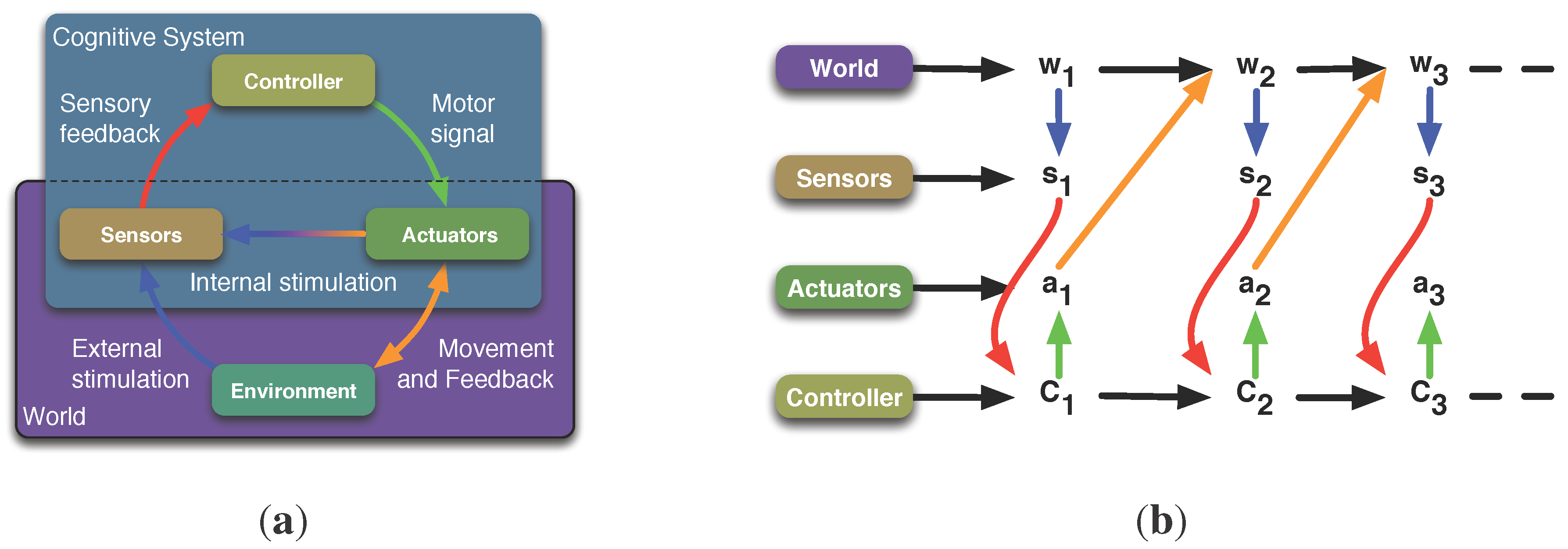
Figure 1.
Schematics and causal graph of the sensori-motor loop. (a) shows the conceptual understanding of the sensori-motor loop. A cognitive system consists of a controller, a sensor and actuator system, and a body that is situated in an environment. The basic understanding is that the controller sends signals to the actuators that affect the environment. Information about the environment and also about internal states is sensed by the sensors, and the loop is closed when this information is passed to the controller. (b) shows the representation of the sensori-motor loop as a causal graph. Here represents the world state at time t. The world is everything that is physical, i.e., the environment and the morphology. The variables and are the signals provided by the sensors or passed to the actuators, respectively. They are not to be mistaken with the sensors and actuators, which are part of the morphology, and hence, part of the world. (a) Schematics of the sensori-motor loop; (b) Representation of the sensori-motor loop as a causal graph.
![Entropy 15 01887 g001]()
The distinction between intrinsic and extrinsic is also captured in the representation of the sensori-motor loop as a causal or Bayesian graph (see
Figure 1(b)). The random variables
C,
A,
W, and
S refer to the controller, actuator signals, world and sensor signals, and the directed edges reflect causal dependencies between the random variables (see [
18,
20,
21]). Everything that is extrinsic is captured in the variable
W, whereas
S,
C, and
A are intrinsic to the system. The random variables
S and
A are not to be mistaken with the sensors and actuators. The variable
S is the output of the sensors, which is available to the controller or brain, the action
A is the input that the actuators take. Consider an artificial robotic system as an example. Then the sensor state
could be the pixel matrix delivered by some camera sensor and the action
could be a numerical value that is taken by some motor controller to be converted in currents to drive a motor.
Throughout this work, we use capital letter (
X,
Y, …) to denote random variables, non-capital letter (
x,
y, …) to denote a specific value that a random variable can take, and calligraphic letters (
,
, …) to denote the alphabet for the random variables. This means that
is the specific value that the random variable
X can take a time
, and it is from the set
. Greek letters refer to generative kernels,
i.e., kernels that describe an actual underlying mechanism or a causal relation between two random variables. In the causal graphs throughout this paper, these kernels are represented by direct connections between the corresponding nodes. This notation is used to distinguish generative kernels from others, such as the conditional probability of
given that
was previously seen, denoted by
, which can be calculated or sampled, but which does not reflect a direct causal relation between the two random variables
and
(see
Figure 1(b)).
We abbreviate the random variables for better comprehension in the remainder of this work, as all measures consider random variables of consecutive time indices. Therefore, we use the following notation. Random variables without any time index refer to time index t and hyphened variables to time index . The two variables refer to and .
We have now defined the conceptual framework in which we will derive the measures for morphological computation. This is done in the next section, which starts with an overview.
3. Measuring Morphological Computation
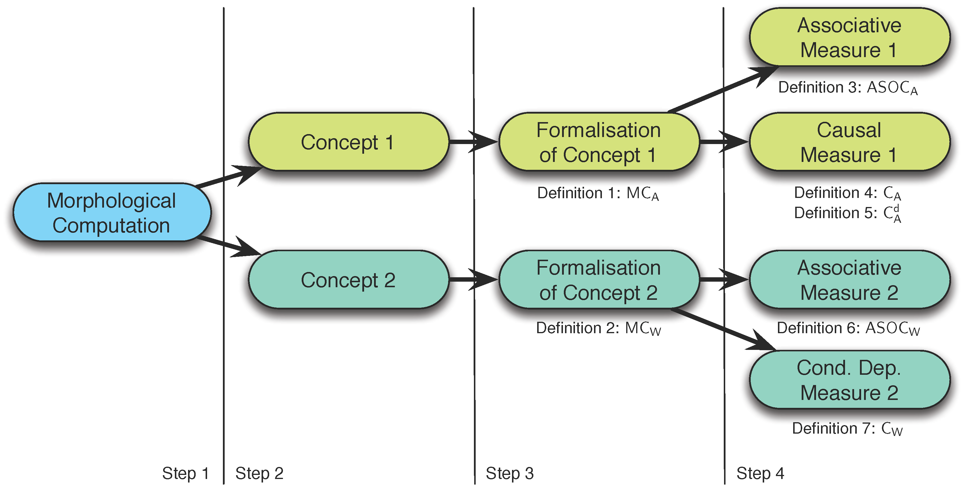
We will derive the measures for morphological computation in four steps (see
Figure 2):
Descriptive definition of morphological computation.
Framing of two concepts that follow from step 1.
Formal definition of the two concepts given in step 2.
Intrinsic adaptations of the definitions given in step 3.
The fourth step is required because the two definitions given in the third step require information about the world state W, which is generally not available. This will be discussed in detail later in this section.
Figure 2.
Outline of the third section of this work, in which the measures for morphological computation are derived. The first step is to provide a description of morphological computation. From this description two concepts are presented in the second step, which are then formalised in the third step. The last step adapts the formalisations to measures that operate on intrinsically available information only.
3.1. Morphological Computation
We understand morphological computation as the contribution of the morphology and environment to the overall behaviour of an embodied system. This implies that morphological computation must be studied in the sensori-motor loop, as it is the result of the interaction of the controller, morphology and environment.
Measuring morphological computation means that an observer has recorded the relevant data of an embodied agent’s behaviour of interest and post-hoc asks the question how much morphological computation was present in the recoded sequence.
Measuring morphological computation does not mean to capture the complexity or the quality of a behaviour. These are aspects of the behaviour of cognitive systems, which are not handled by our measures.
3.2. Concepts of Measuring Morphological Computation
In the following, we assume that an embodied agent is well-captured by the sensori-motor loop as it was presented in the previous section (see
Figure 1). Explicitly, we will use the term world in the way it was defined above, as the system’s morphology and
Umwelt.
Generally speaking, morphological computation is the effect of the current world state
W on the next world state
, which is not assignable to the action
A. Given the sensori-motor loop as we have defined it above (see
Figure 1), this cannot be measured in isolation, as there is a path from
W to
that goes through the agent. Hence, we need to measure the effect of the action
A on the next world state
so that we are able to deduce the effect of
W on
that does not include the pathway over
A. This has two implications. First, the resulting value of such a measure is not an absolute value per se. In fact, it can only be measured as the relation of the two effects
and
. Second, there are two ways of comparing the effects.
The first method of measuring morphological computation assumes that the next world state
is only determined by the current world state
W, which is equivalent to assuming maximal morphological computation. Any measured effect of the action
A on the next world state
displays itself in a reduction of the resulting measurement. This is summarised in the following concept:
Concept 1 (Negative effect of the action) Given a behaviour of interest of an embodied system, the amount of morphological computation is inversely proportional to the contribution of the actions of the system to the overall behaviour.
This concept relates to control-dependent punishments discussed in literature to achieve high morphological computation (e.g., [
22]).
The second method of measuring morphological computation assumes that the next world state
is only determined by the current action
A, which is equivalent to assuming no morphological computation. Any measured effect of the current world state
W on the next world state
displays itself in an increase of the resulting measurement. This is summarised in the following concept:
Concept 2 (Positive effect of the world) Given a behaviour of interest of an embodied system, the amount of morphological computation is proportional to the contribution of the world to the overall behaviour.
3.3. Formalising the Concepts
The next step is to formalise the two concepts presented above. The causal diagram (see
Figure 1(b)) shows that the world kernel
captures the influence of
W and
A on
. Therefore, it is the basis for our further considerations. If the action
A has no effect on the next world state
, then the world kernel reduces to
and we would state that the system shows maximal morphological computation. Analogously, if the world state
W has no influence on the next world state
,
i.e.,
, we would state that the system shows no morphological computation. Measuring the differences of the world kernel to the two conditional probability distributions
and
leads us to the formalisations of the two concepts discussed above. The Kullback–Leibler divergence measures the differences of two probability distributions [
23] and applying it to our scenario gives us the definitions for the two concepts. Their formalisations are given below, such that the value zero refers to no morphological computation and one refers to maximal morphological computation.
Definition 1 (Morphological Computation as negative effect of the action) Let the random variables denote the action, the current and the next world state of an embodied agent, which is described by the causal diagram shown in Figure 1(b). The quantification of the morphological computation as the negative effect of the action on the behaviour is then defined as Definition 2 (Morphological Computation as positive effect of the world) Let the random variables denote the action, the current and the next world state of an embodied agent, which is described by the causal diagram shown in Figure 1(b). The quantification of the morphological computation as the positive effect of the world on the behaviour is then defined as The Kullback–Leibler divergence used in the first measure
can also be rewritten as the conditional mutual information
, which is related to the concept of empowerment [
24]. The latter is defined as
and denotes how empowered an embodied agent is in a specific state of the environment. Morphological computation is correlated with a low influence the influence of the action
A on the next world state
, whereas empowerment requires the maximisation of the influence of the action on the next world state. Maximising morphological computation therefore minimises the empowerment and vice versa. One may speculate that both concepts could be used as balancing forces to find the optimal amount of control for an embodied system.
Both definitions given above require full access to the world states W and . This is undesired for two reasons. First, it limits the applicability of the measure to systems of low complexity that live in the domain of simple grid-world environments. This contradicts our interest in presenting measures that can be used to analyse natural or non-trivial artificial cognitive systems. Second, we believe that the measures derived here may model an intrinsic driving force in the context of guided self-organisation of embodied systems. Hence, we require that any measure must operate on intrinsically available information only. The resulting intrinsic measures are presented below, in the order of the concepts they relate to. The next section lists the four measures without discussing them in detail. They are evaluated and discussed in the subsequent sections.
3.3.1. Concept 1, Associative Measure
The first measure that operates on intrinsic information only is the canonical adaptation of the first definition to the intrinsic perspective. It must be mentioned here that the sensor states
S and
are understood as the intrinsically available information about the external world. Hence, the conditional probability
refers to the intrinsically available information about
.
Definition 3 (Associative measure of the negative effect of the action) Let the random variables denote the action, the current and the next sensor state of an embodied agent, which is described by the causal diagram shown in Figure 1(b). The quantification of the morphological computation as an associative measure of the negative effect of the action is then defined as:
The Kullback–Leibler divergence used in the definition of
(see Def. 3) is also known as the transfer entropy of
A on
S [
25] and it was investigated in the context to quantify the informational structure of sensory and motor data of embodied agents [
26].
3.3.2. Concept 1, Causal Measure
The second measure that follows the first concept is based on measuring the causal information flow of the sensor and action states
on the next sensor state
. To simplify the argumentation, we first consider a reactive system (see
Figure 3(b)). The measure will then also be presented and discussed for non-reactive systems, as both cases result in different measures. The idea for this measure is captured in the
Figure 4. Please keep in mind that the sensor states
S and
are here understood as internally available information about the system’s
Umwelt. The causal information flow from
S to
, denoted by
, includes the information that flows from
S to
over all pathways. This explicitly includes the information flow from
S to
over the action
A (see
Figure 4(a)). Morphological computation is here understood as the causal information flow from
S to
excluding the causal information flowing from the action
A to
(see
Figure 4(c)). Hence, we need to subtract the causal information flow from
A to
, denoted by
(see
Figure 4(b)), to exclude it from
such that we receive the causal information flow that goes from
S to
without passing
A, denoted by
(see
Figure 4(c)).
Figure 3.
Reactive system. In the context of this work, a reactive system is defined by a direct coupling of the sensors and actuators. There is no form of memory present in the system. (a) Schematics of the sensori-motor loop for a reactive system; (b) Representation of the sensori-motor loop for a reactive system as a causal graph.
Figure 4.
Visualisation of the causal measure
. The causal graph used in (
a), (
b) and (
c) is the reduction of sensori-motor loop shown in
Figure 3(b) to two consecutive time steps. (
a) shows that the causal information flow
measures all causal information from
S to
, including the information that flows over
A. (
b) shows that the causal information flow
only captures the information flowing from
A to
. Both can be used to approximate the causal information from
S to
that does not pass through
A, denoted by
, as shown (
c). (
a)
; (
b)
; (
c)
.
According to the general theory [
27], we talk about identifiable causal effects if they are computable from observational data. We stated earlier that we are interested in intrinsic measures. Hence, we require that the causal effects are identifiable from observational data that are intrinsically available to the agent. We refer to this type of identifiability as
intrinsically identifiable. In our previous work [
28], we showed that the causal effects of
S on
and of
A on
are intrinsically identifiable by the following conditional probability distributions:
These distributions need to be explained. The notation
(also denoted by
refers to probability of measuring
x when the state of
Y was set by intervention to
y [
27]. Explicitly, this means that intervention is generally required in order to determine causation. Therefore, it is important to note that the equations above (see Equations
3 and Equation
4) allow us to determine the causal effects
without any intervention. An agent can act in the sensori-motor loop and from its observation determine, e.g., the causal effect of its actions
A on the its next sensor states
(for a discussion, see [
28]). From the two probability distributions given in the Equations (
3) and Equation (
4) we can construct the two required causal information measures for
and
(see also [
21]). The derivations for both measures are given in the appendix (see
Section A.1). The resulting equations are given by
The difference
is always negative (see Equation (58) in
Section A.1), and hence, the resulting measure is given by the following definition.
Definition 4 (Causal measure of the negative effect of the action for a reactive system) Let the random variables denote the action, the current and the next sensor state of a reactive embodied agent, which is described by the causal diagram shown in Figure 1(b). The quantification of the morphological computation as a causal measure of the negative effect of the action is then defined as: The causal information flow
is so far not shown to be intrinsically identifiable for non-reactive systems [
28]. Therefore, we consider the causal information flow from the internal controller state
C to the next sensor state
(see
Figure 1(b)). This is valid because
C represents the entire history of the system and therefore also the internal representation of the entire history of the world. All further calculations are analogous to the previous case (see also [
28] for a discussion) and lead to the following definition.
Definition 5 (Causal measure of the negative effect of the action for a non-reactive system) Let the random variables denote the action, the controller and the next sensor state of a non-reactive or deliberative embodied agent, which is described by the causal diagram shown in Figure 1(b). The quantification of the morphological computation as a causal measure of the negative effect of the action is then defined as: The last definition (see Def. 5) is given for the reason of completeness only. Morphological computation is mainly discussed in the context of behaviours that are well-modelled as reactive behaviours (e.g., locomotion). To the best of our knowledge, it has so far not been discussed in the context of non-reactive or deliberative behaviours. Therefore, the first definition of the causal measure (see Def. 4) suffices for all currently discussed cases of morphological computation in the field of embodied artificial intelligence.
This concludes the measures of the first concept, in which morphological computation is calculated inversely proportional to the influence the action A has on the next world state . The next section discusses the measures for morphological computation in which it is calculated proportionally to the effect the world has on itself.
3.3.3. Concept 2, Associative Measure
Analogous to the associative measure of the first concept, the associative measure of the second concept adapts the Definition 2 to the intrinsic perspective by replacing W by S and by . This leads to the following definition.
Definition 6 (Associative measure of the positive effect of the world) Let the random variables denote the action, the current and the next sensor state of an embodied agent, which is described by the causal diagram shown in Figure 1(b). The quantification of the morphological computation as an associative measure of the positive effect of the world is then defined as: The next measure approximates the dependence of the next world state on the current world state W solely based on the internal world model .
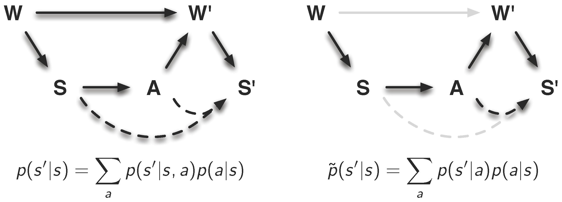
3.3.4. Concept 2, Conditional Independence
The idea of this measure is to calculate how much the conditional probability distribution
estimated from the recoded data differs from the assumption that the world did not have any effect on itself, denoted by the conditional probability distribution
. The
Figure 5 shows the difference between the two conditional probability distributions graphically. The following equations show how they can be calculated from the observed data.
The measure is then defined as the Kullback–Leibler divergence of
and
.
Definition 7 (Conditional dependence of the world on itself) Let the random variables denote the action, the current and the next sensor state of an embodied agent, which is described by the causal diagram shown in Figure 1(b). The quantification of the morphological computation as the error of the assumption that the next world state is conditionally independent of the previous world state is then defined as:
Figure 5.
Visualisation of the conditional independence measure . The left-hand side shows how the conditional probability distributions can be calculated from the world model and the policy . The right-hand side shows how changes, if one assumes that the world does not influence itself (gray arrow between W and ), and if this is reflected in the internal world model (gray arrow between S and ). This difference between and is a measure for morphological computation
This concludes the presentation of definitions of morphological computation measures. The next section discusses their relation to the Information Bottleneck Method [
14].
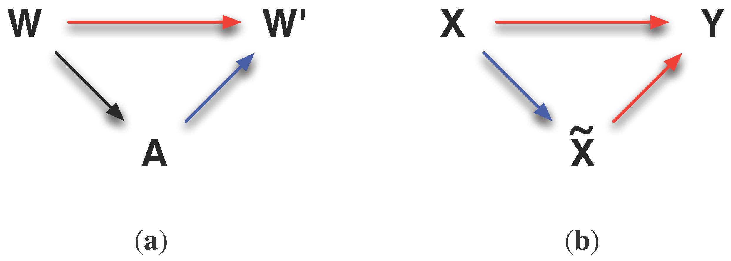
3.4. Relation to the Information Bottleneck Method
We will discuss the relation of morphological computation to the Information Bottleneck Method by Tishby
et al. [
14] along with the two graphs shown in
Figure 6. The graph on the left-hand side (see
Figure 6) shows how we understand morphological computation. It is present if the current world state
W has a high influence on the next world state
(denoted by a red arrow) and the current action
A has a low influence on the next world state
(denoted by a blue arrow). Hereby, it is not relevant how much the world has influenced the action (denoted by a black arrow).
The Information Bottleneck Method is visualised in the
Figure 6. Here, the influence of the world on the action is minimised and the influence of the action on the next world state is maximised. The action
A is the bottleneck variable
(see
Figure 6) for the relevant information that is passed through the world. This appears connected for the following reason. Conceptually speaking, reducing the required alphabet in
A to still maintain the information the world carries about itself is related to the notion of morphological computation, as it means that only a few actions should be chosen by the agent to maintain the behaviour. Formally, the two concepts (Information Bottleneck and morphological computation) are not easily aligned. The Information Bottleneck Method requires to minimise the Kullback–Leibler divergence
(see e.g., Equation (27) in [
14]), whereas morphological computation is defined to minimise the Kullback–Leibler divergence
(see Def. 1) or to maximise the Kullback–Leibler divergence
(see Def. 2). Currently we could not solve this contradiction, but we believe that it should be followed, as it could unify the presented concepts
and
.
Figure 6.
Visualisation of the relation of the concepts to the Information Bottleneck Method. (a) shows the general concept of morphological computation. The world states are highly correlated (red arrow), whereas the world and action are only weakly correlated (blue arrow). (b) shows the concept of the Information Bottleneck Method. The difference is that a strong correlation between the action A and and a weak correlation between W and A are required. For a discussion, please read the text below. (a) Concept of morphological computation; (b) Concept of the Information Bottleneck Method.
This concludes the presentation and discussion of the two concepts, their formalisations, and the resulting four measures that rely on internal variables only. The next step in this work is to evaluate how these different measures behave when they are applied to experiments. This is done in the next section.
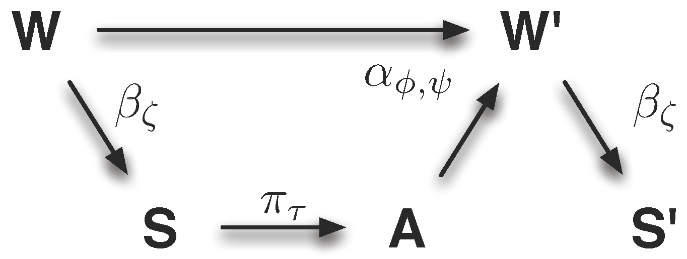
4. Experiments
This section applies the morphological computation measures to two different experiments. The first experiment is a simplified parameterisable model of the one-step sensori-motor loop for reactive systems (see
Figure 3(b)). The model is defined by the four transition maps
,
,
, and
. For each map, the indices refer to its parameters. Hence, the entire model is parameterised by five parameters, of which two are kept constant in the experiments below.
The second experiment is designed as a minimal physical system that allows a transition between the Dynamic Walker [
29] and a classically controlled humanoid.
Both experiments use reactive systems for the reason of simplicity only. This does not mean that all measures are limited to reactive systems. In particular, the two concepts and and the intrinsic adaptations , , and make no assumptions on the type of control. Only , which is used in the following experiments, explicitly requires a reactive control.
4.1. Binary Model Experiment
In the introduction to this paper, it was stated that the measures presented in this work should be applicable to biological systems. In the previous section (see
Section 3), it was stated that the measures should not operate on the world state
W, also because it is not accessible for any example other than simple toy worlds. This section now evaluates the two concepts and four measures based on such a simple toy world example. This might appear as a contradiction to the previous statements, and therefore, the application of the measures to this model needs a further explanation.
In order to understand how the measures differ and in which aspects they are alike, it is best to analyse them under a fully controllable setting. Using real robots only allows to fully control a very limited set of parameters of the entire system, namely the parameters of the policy and partially those of the embodiment. This improves only slightly in simulated robotics, depending on the chosen implementation. These uncontrollable or hidden parameters require robustness of the applied methods and are one of the main arguments for favouring virtual or real robots over grid world environments. The goal of this section is different. Here, we want to validate the measures by controlling the influence of the world on itself in addition to controlling the systems parameters. Therefore, it is necessary to choose an experiment that allows us to fully control every aspect of the sensori-motor loop, explicitly including the world transition kernel . The next section will then validate the measures in a more realistic experiment.
The minimalistic model discussed in this section is shown in
Figure 7 and is defined by the following set of equations:
where all random variables are from the same binary alphabet,
i.e.,
. The model is parametrisable by the variables
, which control how deterministic the kernels are. If we consider the policy
, which is controlled by the parameter
μ, then we see from Equation (22) that
results in
for all
. The policy is completely random, because both actions
and
occur with equal probability, independent of the current sensor value
s. On the other hand, if we set
, then the policy changes to a Dirac measure on the sensor and actuator states,
i.e.,
, where
if
and zero otherwise. The parameter
μ allows a linear transition between these two cases.
For simplicity, but without loss of generality, the following two assumptions are made. First, it is assumed that all world states
occur with equal probability,
i.e.,
. Furthermore, we assume a deterministic sensor,
i.e.,
, which means that the sensor is a copy of the world state. The first assumption does not violate the generality, because it only assures that the world state itself does not already encode some structure, which is propagated through the sensori-motor loop. Second, in a reactive system, as it is shown in
Figure 7, the sensor state
S and
A could be reduced to a common state, with a new generative kernel
. Hence, keeping one of the two kernels deterministic and varying the other in the experiments below does not affect the generalisation properties of this model. This leaves three open parameters
, and
μ, against which the morphological computation measures are validated (see
Figure 9,
Figure 10 and
Figure 11). To be able to understand if the plots validate the measures, it is necessary to understand how the parameters affect the morphological computation in this model. To simplify the argumentation, it is first assumed that the policy is completely random (
), and hence, the action
A is independent of the previous world state
W (this assumption is dropped below). What follows is that the world transition kernel
(see Equation 35) can be divided into four cases (see
Figure 8), which are classified by the effect of
φ and
ψ on the morphological computation. To understand how the parameters affect the measure, they are first discussed with respect to the world kernel
. This is then related to how the Kullback–Leibler divergences used in the two definitions (see Def. 1 and Def. 2) are affected. The analysis is conducted with respect to the two concepts
and
. It will start with the two unambiguous cases. The intrinsic measures are discussed later in this section.
Figure 7.
Visualisation of the binary model. This figure shows the causal graph that is used in the binary model experiment (see text below). It is the graph representing the single step sensori-motor loop of a reactive system, where the indices of the transition maps refer to their parametrisation.
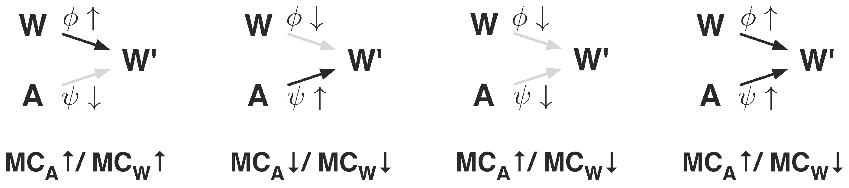
Figure 8.
Visualisation of the four discussed cases of the world model. High values are indicated by an arrow pointing upwards (↑), and low values with an arrow pointing downwards (↓), i.e., refers to the case where and , resulting in a high influence of and low influence of . The figures are discussed in the text below.
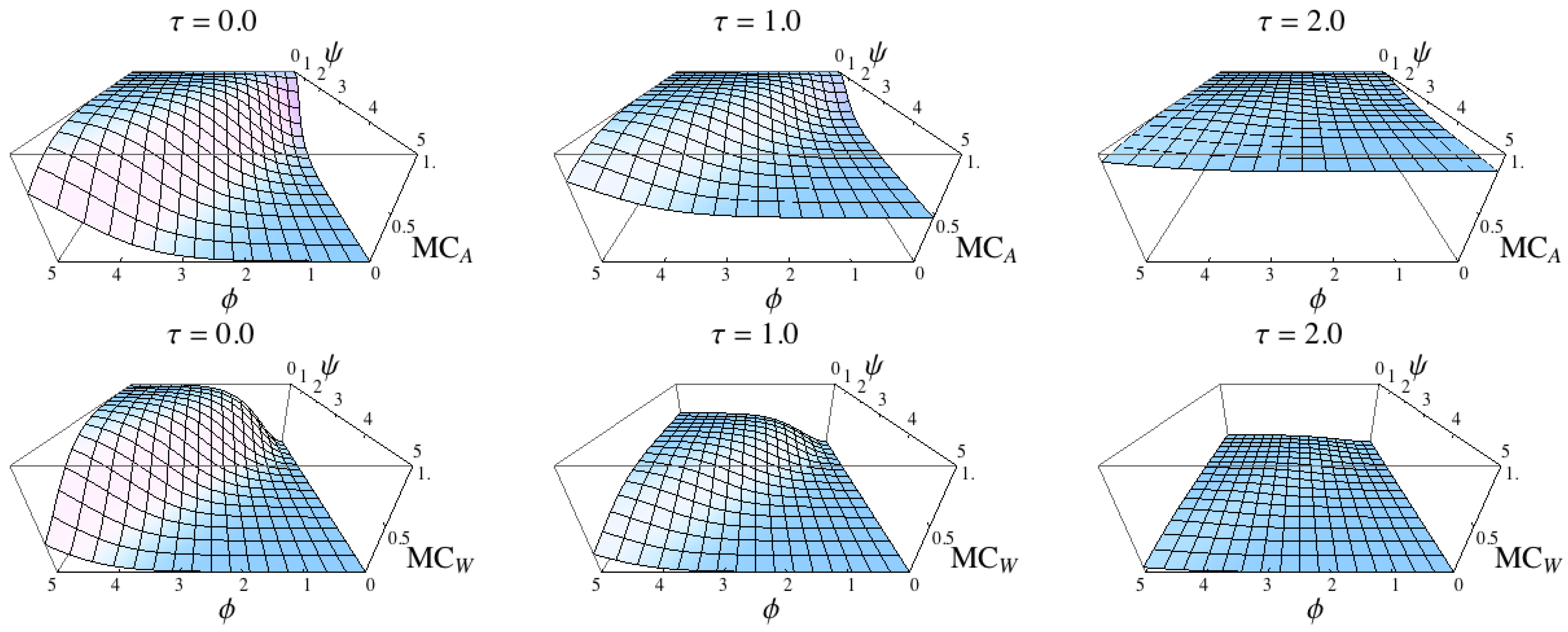
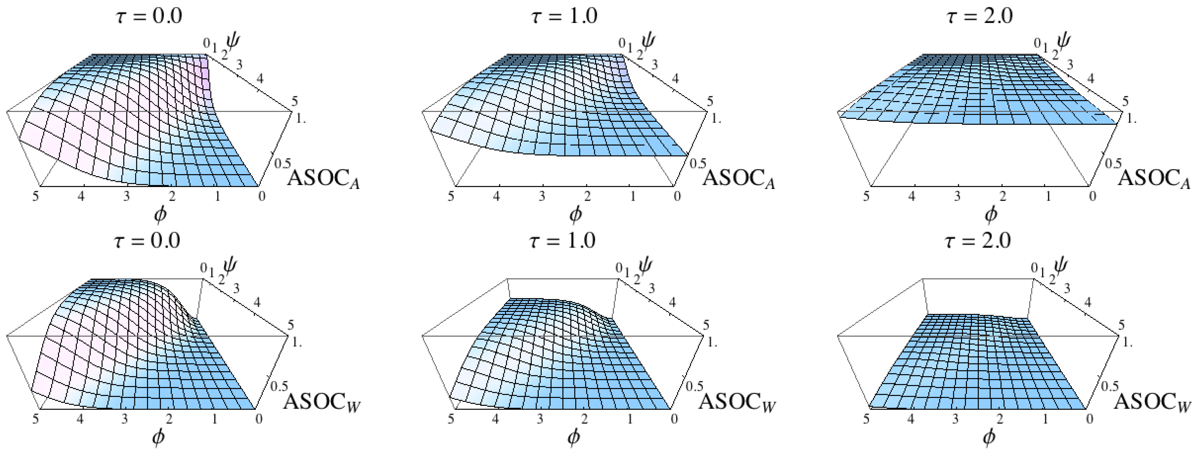
Figure 9.
Numerical results for the measures and and the binary model. The three figures in the first row show the results for with increasingly deterministic policy π (from left to right). The second row shows the results for , also with increasingly deterministic policy. For all plots, the base axes are given by world kernel parameters ψ and φ. The plots confirm the considerations discussed in the text below.
Figure 10.
Comparison of the two measures
and
. The results confirm that the measures are intrinsic adaptations of the measures
and
(see
Figure 9).
Figure 10.
Comparison of the two measures
and
. The results confirm that the measures are intrinsic adaptations of the measures
and
(see
Figure 9).
1st Case: , . This case refers to a world that is only influenced by the last world state, as the world kernel
reduces to a Dirac measure on the current and next world state (see
Figure 8):
The result is a high measured morphological computation for both measures
and
, as
, and hence,
and
are both maximal.
Figure 11.
Comparison of the two measure
and
. The results confirm the measures are intrinsic adoptions of the measures
and
(see
Figure 9).
Figure 11.
Comparison of the two measure
and
. The results confirm the measures are intrinsic adoptions of the measures
and
(see
Figure 9).
2nd Case: , . This case refers to a world that is only influenced by the last action, as the world kernel
reduces to a Dirac measure on the action and next world state (see
Figure 8):
The result is a low measured morphological computation for both measures
and
, as
, and hence,
and
are both minimal.
3rd Case: , . This case refers to a world in which the next world state is independent of the previous world state and the previous action, which is described by
The two measures
and
give different results, because the two quantifications
and
are both zero. Consequently, the two measures lead to
and
.
4th Case: , . This case is a mixture of all previous cases, as the world behaves according to
The fourth case is similar to the third case if the world state W is not equivalent to the action A, because in this case the next world state is independent of both. We saw from the third case that this leads to and . If the action A and the world state W are equal, the first measure reduces the amount of morphological computation, whereas the second measure increases the amount of morphological computation, leading to and .
To complete the analysis of the model before the numerical results are discussed, the assumption of a random policy is dropped. We now assume a fully deterministic policy (
). In this case, the policy reduces to a Dirac measure on the world and action state, as the sensor state is a copy of the world (
), and therefore,
. It also follows that
. For the two measures, it follows that:
The effect that a deterministic policy leads to different results for both concepts will occur in the following experiments. It will be discussed in detail in the next section (see
Section 5).
The four cases are identical with the four corners of the
φ–
ψ plane in
Figure 9, and the four cases are well-reflected in the plots. The plots also visualise the difference of the two concepts for the last two cases (
,
and
,
in
Figure 9).
Next, this section now applies the four intrinsic measures to the binary model. The results are shown for the variations of the three parameters
in
Figure 10 and
Figure 11.
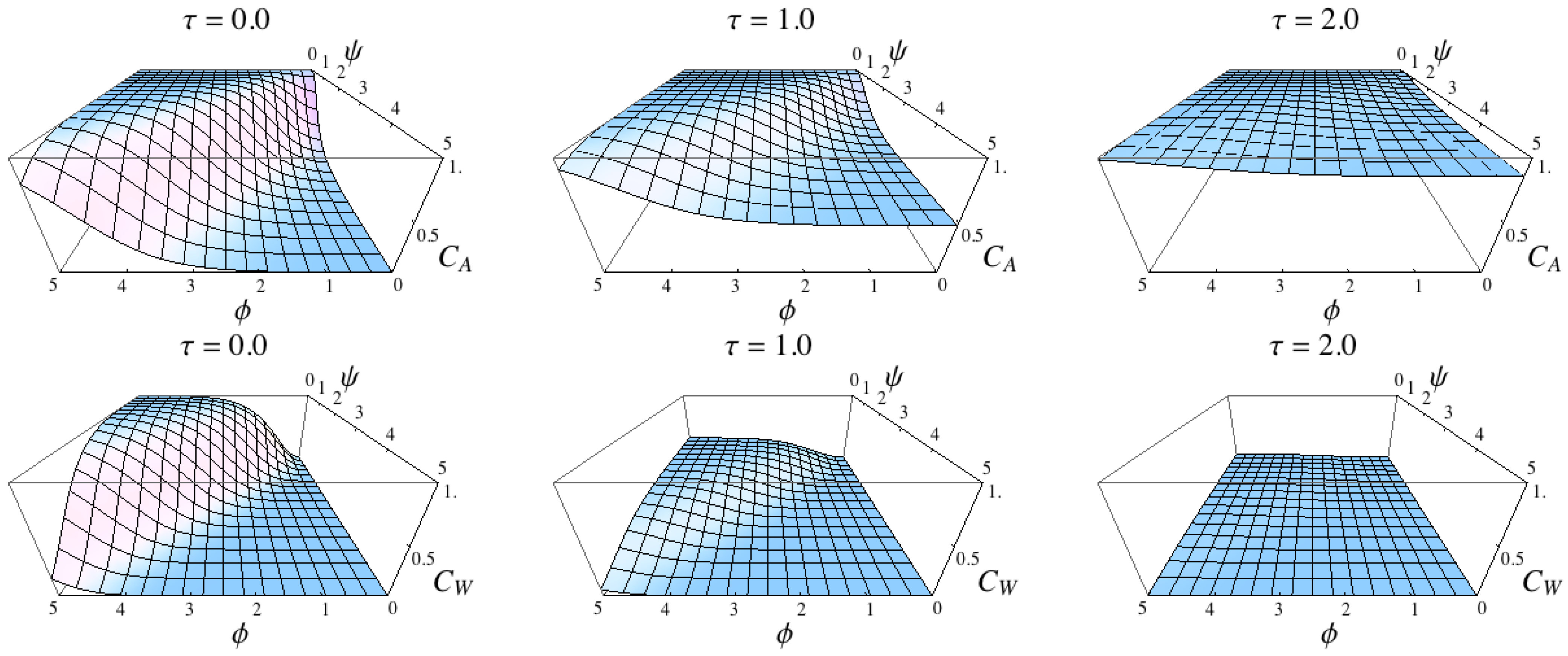
The intrinsic measures require the probability distributions
and
, which can be calculated from the Equations (
20) to (23) in the following way:
The plots reveal that both measures in the first concept and both measures in the second concept show very similar results compared with the formalisation of the concepts (compare
Figure 9 with
Figure 10 and
Figure 9 with
Figure 11). This can be expected because the sensor distribution is equivalent to the world distribution due to Equation (31) and because the sensor kernel was set to be a Dirac measure on the world (
). Nevertheless, the plots show that the intrinsic adaptations of the formalisation of the concepts capture what the concepts specify.
4.2. Rotator
The previous section verified the measures in a very simple yet illustrative binary model of the sensori-motor loop. It was shown that all measures produce the desired output for variations on the transition probabilities of the world and the policy. This section applies the intrinsic measures to an experiment that is inspired by common examples of previously discussed systems that show high and low morphological computation.
The Dynamic Walker [
29] is designed to emulate the natural walking of humans. One characteristic is that only half of the leg movement involved in the walking behaviour is actively controlled by the brain [
30]. It is the stance phase,
i.e., the time during which the foot touches the ground and moves the rest of the body forward, that is fully controlled. The swing phase,
i.e., the time in which the leg swings forward before another stance is initiated, is only partially controlled. One may say that the body lets loose and gravity takes over. This is exactly what the Passive Dynamic Walker highlights, as it only exploits its body and the environment,
i.e., the slope and gravity, to produce a natural walking behaviour.
The world’s most advanced humanoid robot (quoted from [
31]) Asimo is an example of a system that does not show any morphological computation as it is discussed in this work. The trajectory of each part of the morphology is carefully controlled during the stance and swing phase at all times. This is also the reason why the motion of Asimo does not appear natural although it is very smooth.
We are now presenting a simple experiment that allows us to vary the amount of exposed morphological computation between the two examples discussed above. For this purpose we chose a pendulum, which can rotate freely around its anchor point. The task of our controller is to consistently rotate the pendulum clockwise. The Asimo case is approximately given, if the angular velocity of the pendulum is controlled at every instance in time, whereas the Dynamic Walker case is approximated if the angular velocity of the pendulum is only altered for large deviations of the current angular velocity from the target velocity. This will be clearer after the equations have been presented. The pendulum is modelled by the following equation:
where
is the force imposed by the controller (see below),
γ is the friction coefficient,
is the current angle of the pendulum,
m is its point mass that is located from the centre by the length
l. Equation (
36) was numerically solved for
using the NDSolve method of Mathematica 8.0 [
15]. The actions
were modified only for
, and kept constant while Equation (
36) was solved. This refers to a behaviour update frequency of 100 Hz. The controller is defined by the following set of equations:
The function of the controller is explained along the three equations, Equation (
37) to Equation (39). The Equation (
37) adds uniformly distributed noise
to the sensed angular velocity
, which is then presented as sensor value
to the controller. It was discussed in the previous section that a deterministic reactive system prevents the possibility to distinguish between the information flow of
and
as
A becomes a deterministic function of
W, and hence
A and
W are equivalent with respect to our measures. Therefore, noise is added to the sensors such that
is not deterministically dependent on
. Equation (38) determines the strength of the response of the controller as a function of the difference of the sensor value
and the target angular velocity
(see first term in Equation 38). This function is only executed if the difference of the sensor value to the goal is larger than a threshold value
β. Hence, to ensure sensitivity, the threshold value is subtracted from the absolute value of the response (see second term in Equation 38). The third term in Equation (38) ensures a minimal response strength, and hence, a minimal effect of the action
on the next sensor value
.
All parameters shown in Equations (
36)–(
39) were evaluated systematically. The most distinctive results were found for the following values, which is why they were chosen for presentation here:
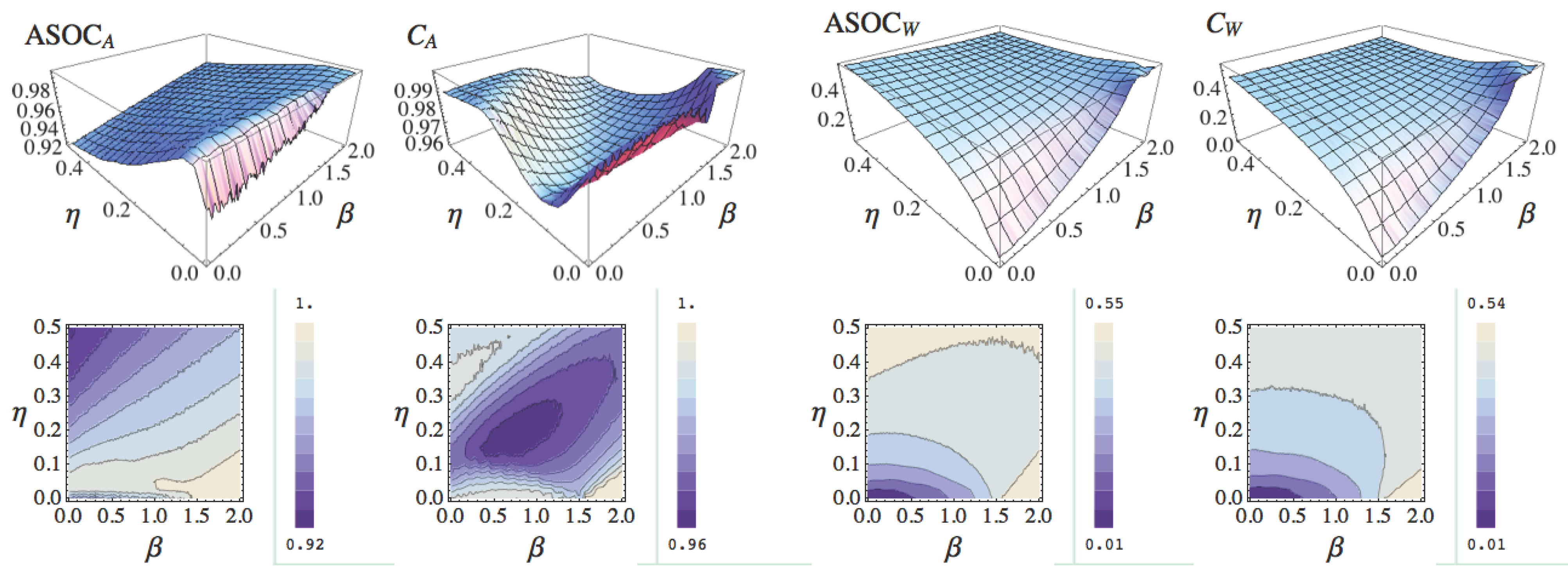
The results are presented in two figures (see
Figure 12 and
Figure 13).
Figure 12 shows three-dimensional plots in which the plane is defined by the noise factor
η and the threshold
β, and for which the height
z is given by the measurements of the denoted measure.
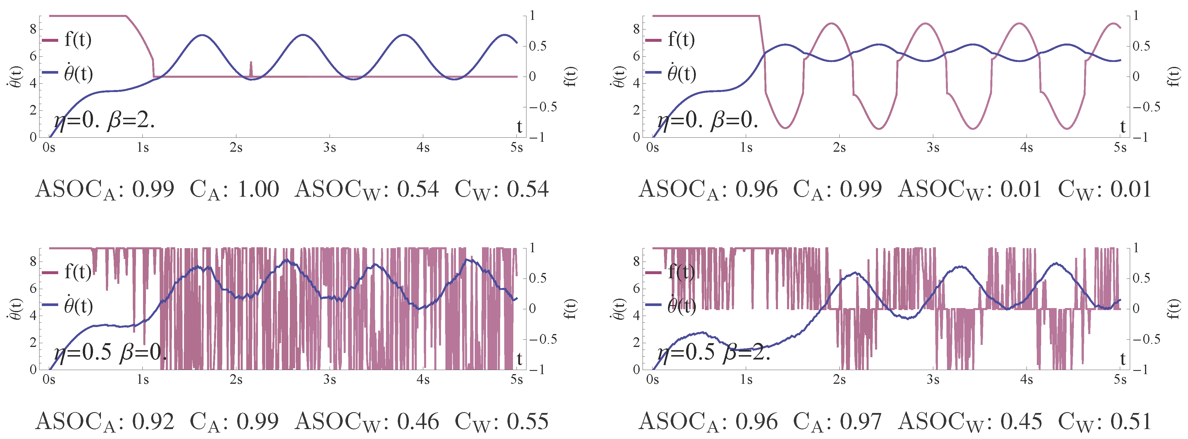
Figure 13 shows the transients of the sensor values
(see Equation
37) and the normalised action
(see Equations 38 and 39) for the four extremal points of the plots in
Figure 12. Therefore, the five plots in
Figure 13 show the transients for the configurations
. The discussion of the results in the following paragraphs refers to these two figures and follows the ordering of the transient plots in
Figure 13. All results were obtained by sampling the world model
, policy
and sensor distribution
from the data stream of 5000 behaviour updates (see Equation
36). The sampling was performed according to [
18] (it is additionally also briefly described in
Section A.2 of the appendix). The sensor values were binned in the interval
and the actions were binned in the interval
with 30 bins each.
The first discussed configuration is
. The transients show a clear picture, as no action of the controller is performed other than
after about 2 seconds. Consequently, for this configuration any measure should result in maximal morphological computation leading to a value close or equal to one, as the inertia, and hence, the world
W is the only cause for the observed behaviour. We see that both measures of the first concept (
and
) deliver a value close or equal to 1 (all values in the
Figure 13 are rounded to the second decimal place and are averaged over 100 runs). The two measures of the second concept (
and
) show their maximal values for this configuration at approximately 0.54 (maximal refers to all configurations shown in
Figure 12). This again highlights the differences of the two concepts. The first concept reduces the amount of morphological computation by the measured effect of the action
A on the next world state
, measured through
, whereas the second concept increases the morphological computation by the measured effect of
W on
, captured by
S and
. This explains why both concepts show different maximal values for this configuration.
Figure 12.
Results of the intrinsic measure in the rotating pendulum experiment. From left to right , , , and . The plane in each plot is defined by the noise η and the threshold parameter β. The values are averaged over 10 runs, for and . The results are discussed in the text below.
Figure 12.
Results of the intrinsic measure in the rotating pendulum experiment. From left to right , , , and . The plane in each plot is defined by the noise η and the threshold parameter β. The values are averaged over 10 runs, for and . The results are discussed in the text below.
Figure 13.
Transients. Please see the legend to each plot and read the text below for a discussion. The values were averaged over 100 runs.
Figure 13.
Transients. Please see the legend to each plot and read the text below for a discussion. The values were averaged over 100 runs.
The second discussed configuration is given by . We expect no morphological computation, because a threshold of means that the pendulum is controlled at every time step t, and no noise on the sensor values means that the action is only dependent on the actual angular velocity . We see that in this case both concepts lead to very different results. The second concept matches our intuition better as both measures ( and ) deliver values close to zero. The measures in the first concept result in values close to one, as the action A is deterministically dependent on the world state W, captured by S, and hence the effect of is fully determined by the effect of . Consequently, in the first concept, the current world state W almost fully determines the next world state , which leads to the high values. We want to point out that there is no preference to any one of the two results. Both seem equally valid at the current stage of the discussion. This is strong evidence that both concepts capture important aspects but that a clear picture cannot be presented yet. We will discuss this in detail in the next section.
The other two configurations show that a noisy controller output is filtered by the inertia of the pendulum, resulting in an angular velocity approximating the target velocity. The amount of noise η increases the measured morphological computation as well as the higher threshold value β. Both results are consistent with our expectations.
5. Discussion
Pfeifer and Scheier [
3] state that
one problem with the concept of morphological computation is that while intuitively plausible, it has defied serious quantification efforts. From the experiments presented in the previous section, we can now understand where this problem rises from. In the context of a deterministic world, a deterministic embodiment and a deterministic reactive policy, one cannot distinguish between the effect of the world
W and the effect of the action
A on the next world state
, as the action
A is given by a deterministic function of
W. Hence, the two states can be subsumed to a single state, which results in the obtained difference of the measures in the two concepts (see Equation 30). We will study this with respect to a
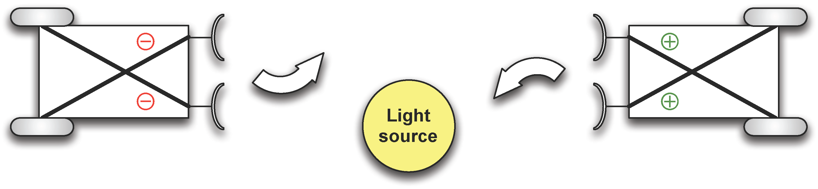
Gedankenexperiment by Braitenberg [
32]. In his book, Braitenberg discusses different vehicles, which show different behaviours due to a very simple sensor-motor coupling. The vehicle 3 is of such kind. It has two sensors that can detect light sources and two actuators with which the system can move and steer. The sensors and motors are cross-coupled (see
Figure 14). Depending on the polarity of the couplings, the vehicle is either attracted or repelled from a light source. For this experiment, the two measures result in
and
. Which one is considered to be correct depends on how the policy is separated from the body. One may argue that the coupling and the coupling strength defines the policy. In this case, one has to conclude that there is low morphological computation, as the next world state is mostly determined by the policy. This favours the measure
. One may also argue that the couplings between the sensors and actuators are of such simplicity, that they can be considered as part of the body, as the sensor signals directly feed to the actuators. In this case, the state of the system is fully determined by the current sensor state, and hence, the world state. This is in favour of the first measure
.
It seems that both concepts capture important aspects of morphological computation but a final answer cannot yet be given here, as the discussion about the Braitenberg vehicle 3 shows.
Another important point must be discussed here. All presented quantifications measure the influence of the world state
W on the next world state
in one way or the other (best seen in
Figure 5). One may argue that measuring morphological computation requires to take the control system into account, as an open-loop control system should show more morphological computation compared with a closed-loop control system, because the morphology becomes more relevant. How closed-loop and open-loop systems relate was first investigated by Touchette and Lloyd [
33], who measured how much information a control system acquires from the environment. That this complementary concept does not capture morphological computation well is shown by the following example. A manufacturing robot working in an industrial assembly line is not associated with high morphological computation, because it is especially constructed and programmed to compensate for any uncontrolled effects resulting from the morphology. The trajectory of the tool is pre-programmed to the extent that any human entering its working space during operation is risking serious injuries. This is because this type of robots are not equipped with sophisticated sensors and mainly controlled in an open-loop paradigm. Morphological computation is the information that the
environment processes as opposed to the information that the
control system acquires [
33] or processes from the environment.
Figure 14.
Braitenberg Vehicle 3. The figure shows two Braitenberg vehicles, each equipped with two light sensors and two actuators. The polarity of the sensor-motor couplings determines the behaviour. The Braitenberg vehicle on the left-hand side is repelled by light, whereas the Braitenberg vehicle on the right-hand side is attracted by light.
We previously discussed the connection of morphological computation to the Information Bottleneck Method. Here we discussed the connection open- and closed-loop control to our measures. Both are dealing with the mutual information of the current world state W and the current action A in different ways. Investigating the connection among the Information Bottleneck Method, Touchette and Lloyd’s approach and morphological computation seems to be a very promising approach to generate new insights about the sensori-motor loop. Unfortunately, it is beyond the scope of this work.
6. Conclusions
This work began with an introduction of morphological computation in the context of embodied artificial intelligence. It was concluded that the complexity of the controller or brain should not be the primary ingredient for a measure of morphological computation. Instead, the influence of the action of an agent and the influence of the last world state need to be compared. Two concepts to measure morphological computation were then discussed and formalised, from which several intrinsic adaptations were derived. The different measures were evaluated in two experiments, which showed the conceptual difficultly in measuring morphological computation. For any fully deterministic reactive system, the influence of the action and the influence of the world are not easily separated, which leads to different results for the two concepts. As this only occurs in this very special case, i.e., when no noise is present in the entire loop, we propose to use the different results as an indication that the observed behaviour may be due to such a deterministic reactive system.
From the derivation of the concepts, it is clear that the world states W and may include not only an individual’s morphology and Umwelt but also those of other agents. Hence, our measures also apply to quantify collective behaviours such as stigmergy, flocking, etc. Discussing this is beyond the scope of this work but subject to future research.
Two concluding remarks will close this work. First, the presented concepts each points to important aspects of morphological computation but are not the final answer. A final measure will have to combine both concepts into one. How this can be done is open to future work. Second, although a definite answer is not yet given, the intrinsic adaptations are good candidates for self-organisation principles. An embodied system should maximise its morphological computation in order to minimise its computational requirements. This may have implications for practical applications in the field of robotics, as the amount of on-board computation and therefore load and energy requirements could be reduced. In first and ongoing experiments we apply the intrinsic measures to the learning of locomotion for a six-legged walking machine in the context of reinforcement learning. The travelled distance is multiplied with the normalised intrinsic measures to give the overall reward. Here, practical advantages of the measures in the second concept seem to be that they start with zero, which means that there is a higher pressure to exploit the morphology, and that they are more sensitive, which was already seen in the rotator experiment presented above.
In conclusion, we state that although not finally answered, the proposed measures already give powerful tools to measure and exploit morphological computation in the context of embodied intelligence.

