1. Introduction
With the promotion of the smart grid concept and the introduction of restructuring into the electric power industry, load forecasting has an even greater importance due to its applications in the planning of demand side management, distributed energy resources, electric vehicles, etc. Many operating decisions rely on accurate short-term load forecasting (STLF), such as generation capacity scheduling, scheduling of fuel and coal purchases, system security analyses, energy transaction planning, etc. It also plays a significant role in the coordination of hydro-thermal systems, generator maintenance scheduling, load flow analysis, etc. The non-linear and stochastic nature of electricity load forecasting is a challenging subject, primarily because of complicated relationships with other factors, such as weather conditions, social activities, seasonal factors, past usage patterns and calendar features. Each of these factors has a significant impact on future load.
Consequently, improving STLF accuracy is crucial for increasing the efficiency of energy systems and reducing operational costs. Complex nonlinear relationships between load and its various influential factors cannot be properly represented by conventional linear models and for that purpose artificial intelligence-based techniques are employed. These methods include: Kalman filters [
1], fuzzy inference [
2], knowledge-based expert systems [
3], artificial neural networks (ANNs) [
4] and support vector machines (SVMs) [
5]. Hybrid approaches are proposed to take advantage of the unique strengths of each method. An adaptive two-stage hybrid network with a self-organized map and support vector machines is presented in [
6]. A hybrid method composed of a wavelet transform, neural network and an evolutionary algorithm is proposed in [
7]. A combined model based on the seasonal ARIMA forecasting model, the seasonal exponential smoothing model and the weighted support vector machines is presented in [
8] with the aim of effectively dealing with the seasonality and nonlinearity shown in the electric load.
In addition to ANNs, which showed a good approximation capability for non-linear functions, SVMs proposed by Vapnik in [
9] are also widely used for load forecasting. However, SVMs are based on the structural risk minimization principle in order to minimize the upper limit of the estimation error, rather than the empirical risk minimization which minimizes the training error used by ANNs. Consequently, by solving the quadric programming (QP) optimization problem, SVMs always manage to achieve the global optimum solution, instead of the possibility of getting stuck in a local optimum like ANN models. This approach, by using nonlinear kernels, leads to a very good generalization performance and sparse solutions. Reformulations of standard SVMs, LS-SVMs defined in [
10], instead of solving the QP problem, which is complex to compute, obtain a solution from a set of linear equations. Therefore, LS-SVMs have a significantly shorter computing time and they are easier to optimize.
In order to provide storage and computational savings and improve the accuracy of the predictions, two different approaches can be applied before training any forecasting model: feature selection and selection of an appropriate subset of instances that are in the training set. Feature selection chooses the most important features, finding an adequate subset of variables in such a way that it is possible to train a more accurate model while reducing the dimensionality of the features space. The selection of instances pulls out instances which do not meet the selection criterion, and thus determines a subset of the initial training data set in such a way that the accuracy of the model increases, but the computational cost and storage requirements are diminished.
Only a few papers have dealt so far with the approach of instance selection for increasing the STLF model accuracy. A method used to forecast electricity prices and load several hours ahead, which used an ANN model with a similar day approach, is presented in [
11]. Therefore, a selection of similar days that represents a trend of load and temperature is performed using the Euclidian norm with weighted factors in order to evaluate the degree of similarity between a forecasted day and previous days. In [
12] a system for power load forecasting using a support vector machine and ant colony optimization is presented. The colony optimization method is employed to process a large amount of data and eliminate redundant information. It is shown that the SVM-learning system performs better when the information preprocessing is based on ant colony optimization. The approach described in [
13] presents a similar day-based wavelet neural network method to forecast tomorrow's load. The key idea is to select a similar day's load as the input load based on the correlation analysis and apply a wavelet to decompose it into a low frequency component and a high frequency component, and then use separate networks to predict the two components of tomorrow's load. The aim of similar day selection was to select the days with the same weekday index, similar weather index and day-of-the-year index to avoid seasonal variations. Only recently has the application of MI for instance selection been proposed in [
14] aiming to remove outliers and noise from highly distorted data sets. The applied algorithm determines the loss of MI with respect to its neighbors in such a way that if a loss of MI is similar to the inputs near the examined instance, then this instance must be included in the training dataset. This approach has proved successful in situations when it is applied to training sets which are artificially distorted by adding noise or outliers.
The work developed in this paper is framed within the instance selection approach with the aim of improving the accuracy of the load forecasting model above all. The MI will be used in order to decide which instances should be included or not in the training data-set, because of its ability to measure the dependence between random variables without prior knowledge of the nature of their underlying relationships. A new methodology for training subset selection is proposed based on the MI computation between initial training set instances and current testing instances. Accordingly, several LS-SVM models based on the proposed methodology have been built for the hourly forecasting of electric load for one day ahead. For each hour of the day for which forecasting is performed, a new training subset is selected, one that fits the current forecasting scenario better. As the experimental results show, in this way significant improvements to the accuracy of forecasting results can be achieved, as well as a great reduction in the training set size.
The rest of the paper is organized as follows:
Section 2 presents the formulation of the MI, describes the method used to compute it and introduces the basic of LS-SVM for regression. In
Section 3, the analysis of the data-set used for methodology testing is given. Then,
Section 4 presents the proposed input selection algorithm and the STLF model. The obtained numerical results are presented and discussed in
Section 5.
Section 6 concludes the paper.
2. Methodology
2.1. Review of Mutual Information
Mutual information is commonly used for measuring dependencies between random variables in a way that does not make any assumptions about the nature of their underlying relationships. Therefore, MI is more powerful in some cases than estimators that only consider the linear relationships between the variables. The MI of two random variables
X and
Y quantifies the information that
X and
Y share. More formally, MI measures how much knowing one variable reduces the uncertainty about the other. The definition of MI is derived from the entropy in information theory. Let us denote
X and
Y as continuous random variables with a joint probability density function
and marginal density functions
and
. The MI between two random variables
X and
Y can be computed as:
The estimation of the joint probability density function (PDF) for a pair (
X, Y) is needed for the computation of MI. The most commonly used methods for PDF estimation are histograms and kernel estimators presented in [
15,
16]. However, they are commonly used with functions of one or two variables because the number of samples needed for the reliable PDF estimation increases exponentially with the number of variables. As a result, the PDF estimator used in this paper is a
k-nearest neighbor (
kNN) based MI estimator, proposed in [
17]. The novelty of this estimator lies in its ability to estimate the MI between two multi-dimensional variables.
Let us consider the set of
N input-output pairs
which are the independent and identically distributed realizations of a random variable
, where
x and
y can be either scalar or vector. For any pair of points
z and
zʹ, the maximum norm is used for the comparison of input-output pairs defined with:
The basic idea is to estimate
I(X, Y) from the average distances in the
X, Y and
Z spaces from
zi to its
k nearest neighbors, averaged over all
zi. Let us denote
the
kth nearest neighbor of
zi. It should be noted that
xk(i) and
yk(i) are the input and output parts of
zk(i) respectively, and thus not necessarily the
kth nearest neighbor of
xi and
yi. Let us define
,
,
. Evidently,
. Subsequently, the number
of points
whose distance from
xi is strictly less than
di are counted, and similarly the number
of points
whose distance from
yi is strictly less than
di are counted. Then,
I(X,Y) can be estimated as presented in:
where
is the digamma function defined as:
and
is gamma function defined by:
Function
satisfies the recursion equation
and
where
is the Euler-Mascheroni constant. The algorithm spends most of the execution time searching for neighbors. When the basic version of
kNN search is implemented, two nested loops are needed through all the points, which gives an algorithm complexity
O(
N2). This paper implements this type of estimator which is one of the two proposed in [
17]. This type of MI estimator depends on the value chosen for
k, which controls the bias-variance tradeoff. As it is recommended in [
18] a mid-range value for
k = 6 will be used.
2.2. A Review of Least Squares Support Vector Machine
Least squares support vector machines, as a reformulation of SVMs, are commonly used for function estimation and for solving non-linear regression problems. The main property of these methods is that they obtain a solution from a set of linear equations instead of solving QP problem, as in SVMs. Therefore, LS-SVMs have a significantly shorter computing time and they are easier to optimize.
Let us consider a given training set
with inputs
and outputs
. The following regression model can be built by using a non-linear mapping function
which maps the input space into a high-dimensional feature space and constructs a linear regression in it. The regression model in primal weight space is expressed as:
where
ω represents the weight vector and
b is a bias term.
LS-SVM formulates the optimization problem in primal space presented with:
subject to equality constrains expressed with:
While
ek represents error variables,
γ is a regularization parameter which gives relative weight to errors and should be optimized by the user. In order to solve the optimization problem defined with (7) and (8), it is necessary to construct a dual problem using the Lagrange function. Once the mathematical calculations have been carried out, described in detail in [
10], the following linear system, presented in (9), was obtained:
In (9), , , are Lagrange multipliers, I is an identity matrix and denotes the kernel matrix. Training the LS-SVM is equivalent to computing the inverse of a full N x N matrix, so when it is implemented straightforwardly its complexity is O(N3), where N is the number of training examples.
Once the system defined in (9) is solved, the solutions for α and
b are obtained. It is shown in [
10] that usually all Lagrange multipliers are non-zero, which means that all training data participate in the solution,
i.e. every data point represents a support vector. Compared with SVM, the LS-SVM solution is not sparse.
The resulting LS-SVM model for function estimation in dual form is represented as:
The dot product is known as a kernel function. Kernel functions that satisfy Mercer's condition enable computation of the dot product in a high-dimensional feature space by using data inputs from original space, without explicitly computing .
A commonly used kernel function in non-linear regression problems, one that is employed in this study, is a radial basis function represented as:
where the kernel parameter
σ2 denotes the square of the variance of the Gaussian function, which should be optimized by the user.
When choosing the RBF kernel function with LS-SVM, the optimal parameter combination (γ, σ) should be established on the training set, in order to obtain the solutions for α and b from (9). The optimal values of these parameters are not known in advance for a given problem, and accordingly must be learned from the training set. In this purpose, a grid search algorithm in combination with k-fold cross validation (k = 10) was used in this study. The procedure goes as follows: the training set is randomly subdivided into k disjoint subsets of approximately equal size and the LS-SVM model is built k times with the current pair (γ,σ). Each time, one of the k subsets is used as the test set and the other k-1 subsets are put together to form a training set. After k iterations, the average model error is calculated for the current pair (γ,σ). The entire process is repeated with an update of the parameters (γ,σ) until the given stopping criterion (e.g. Mean Squared Error) is reached. The parameters (γ,σ) are updated exponentially in the given range using predefined equidistant steps, according to the grid-search procedure. After obtaining the optimal (γ,σ) combination, values for α and b are obtained from (9), and a LS-SVM regression model is formed according to expressions (10) and (11). Also, it can be noticed that in case of LS-SVM, only two additional parameters (γ, σ) need to be optimized, instead of three (γ, σ, ε) as in SVM.
3. Data analysis
Choosing the appropriate features is the first and one of the most important steps in building a forecasting model. In many related works [
5,
19,
20] feature analyses were done, and their impact on the load forecasting model is explained and analyzed. To select the most valuable features, a load curve analysis and statistical analysis of the load pattern are the most commonly used approaches. In this paper, history load data from the Elia Company are used for method evaluation. The data are publicly available and can be downloaded from [
21]. In
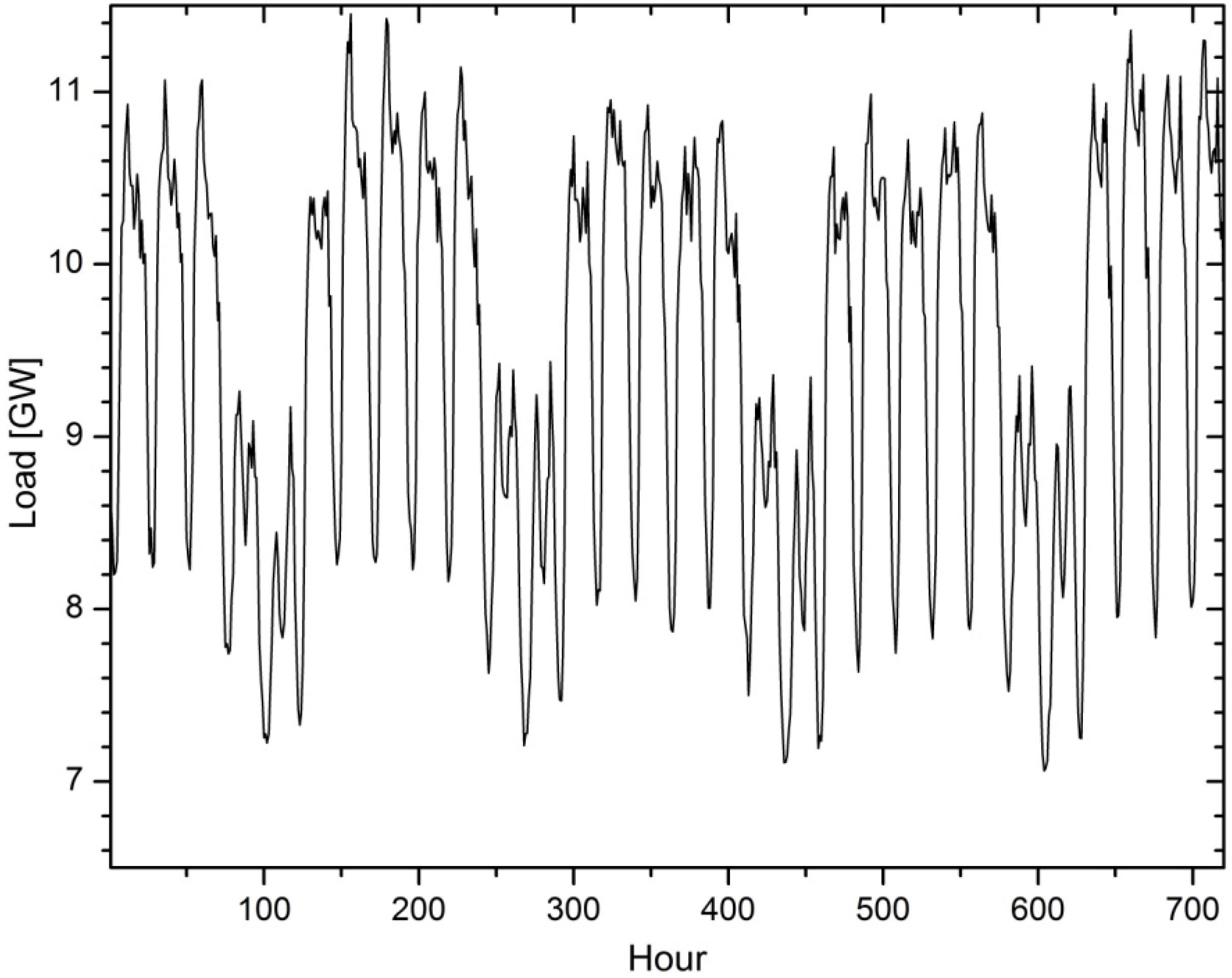
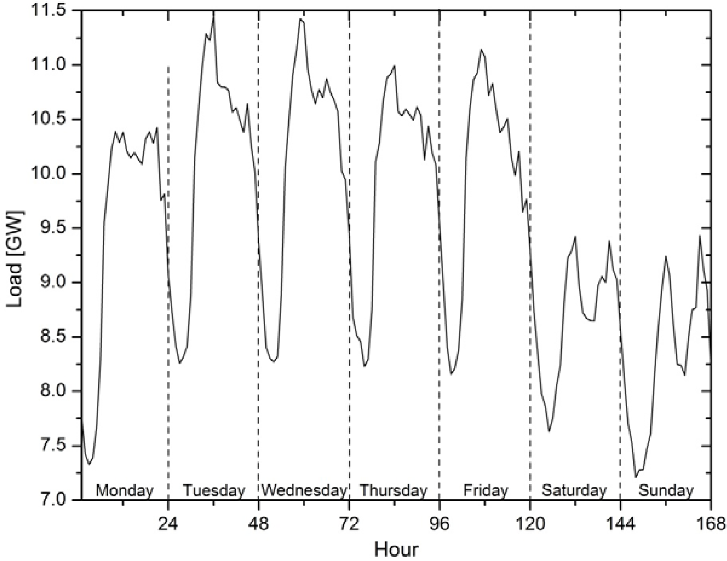
Figure 1, the hourly load curve for one month (September 2010) is shown.
Figure 1.
Hourly load for September 2010.
Figure 1.
Hourly load for September 2010.
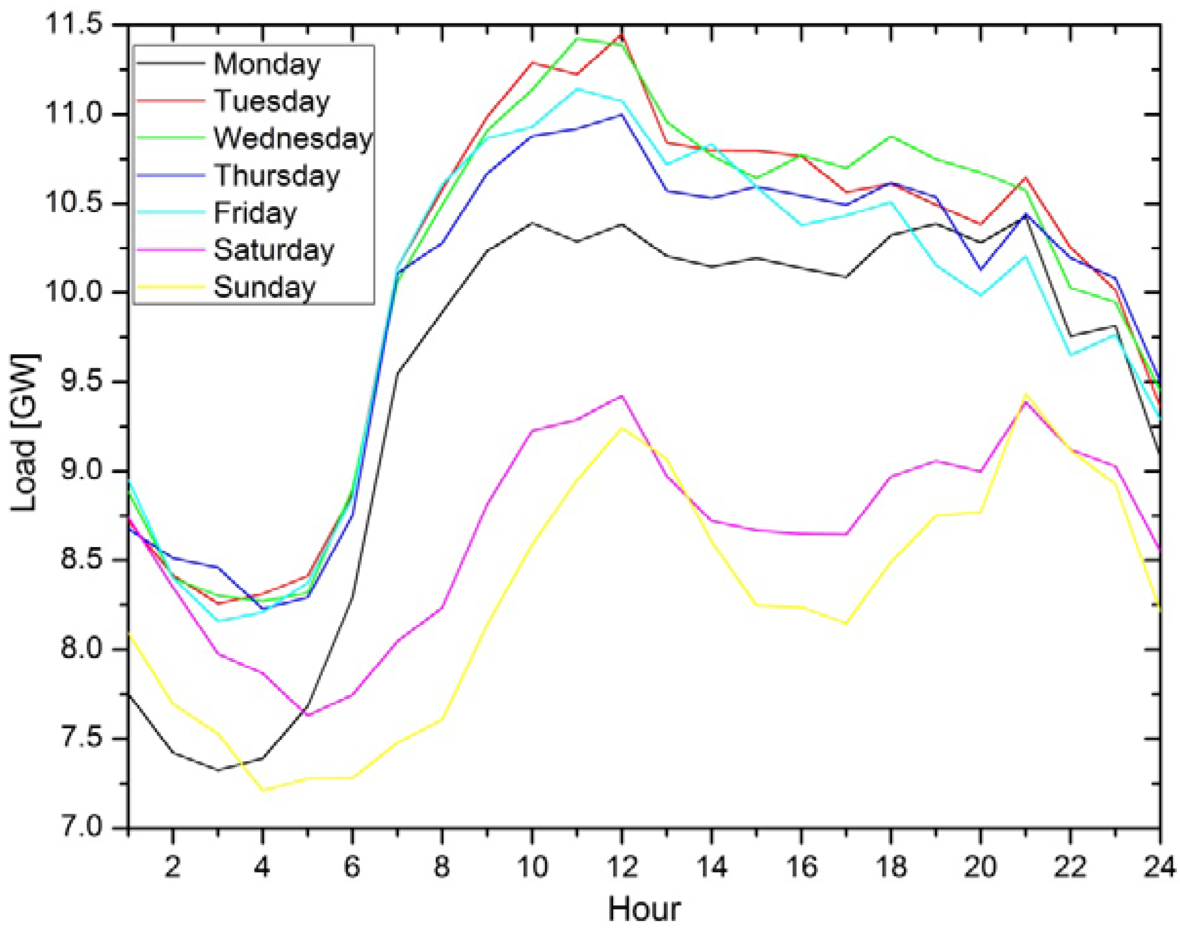
In
Figure 2, the daily load curve during the week is presented. It is obvious that the daily load on work days is greater than the load on weekend days. The reason for this is people's behavior during the week, and this pattern is periodically repeated each week. All this supports using a day of the week for the feature in the model.
Figure 2.
Hourly load during the week.
Figure 2.
Hourly load during the week.
Figure 3 shows the hourly load during the day for each day in one week. This curve is influenced and shaped by people's daily life. The load changes from hour to hour during the day, indirectly following consumer behavior. This brings one more important variable to the feature set, and that is the hour of the day. Also, it can be noticed that the curves have a similar shape but different magnitude from day to day in the week. This also confirms the validity of using the day of the week for the model feature with the aim of mapping this property.
Figure 3.
Hourly load during the day.
Figure 3.
Hourly load during the day.
Past load can also provide useful information for the model about future load fluctuation. Several past hourly loads provide a model with the possibility of recognizing future behavior of the load and giving good load prediction in the next hour. The past load time horizon used in this paper is m=24, i.e., the model uses the last 24 hour loads from the prediction moment.
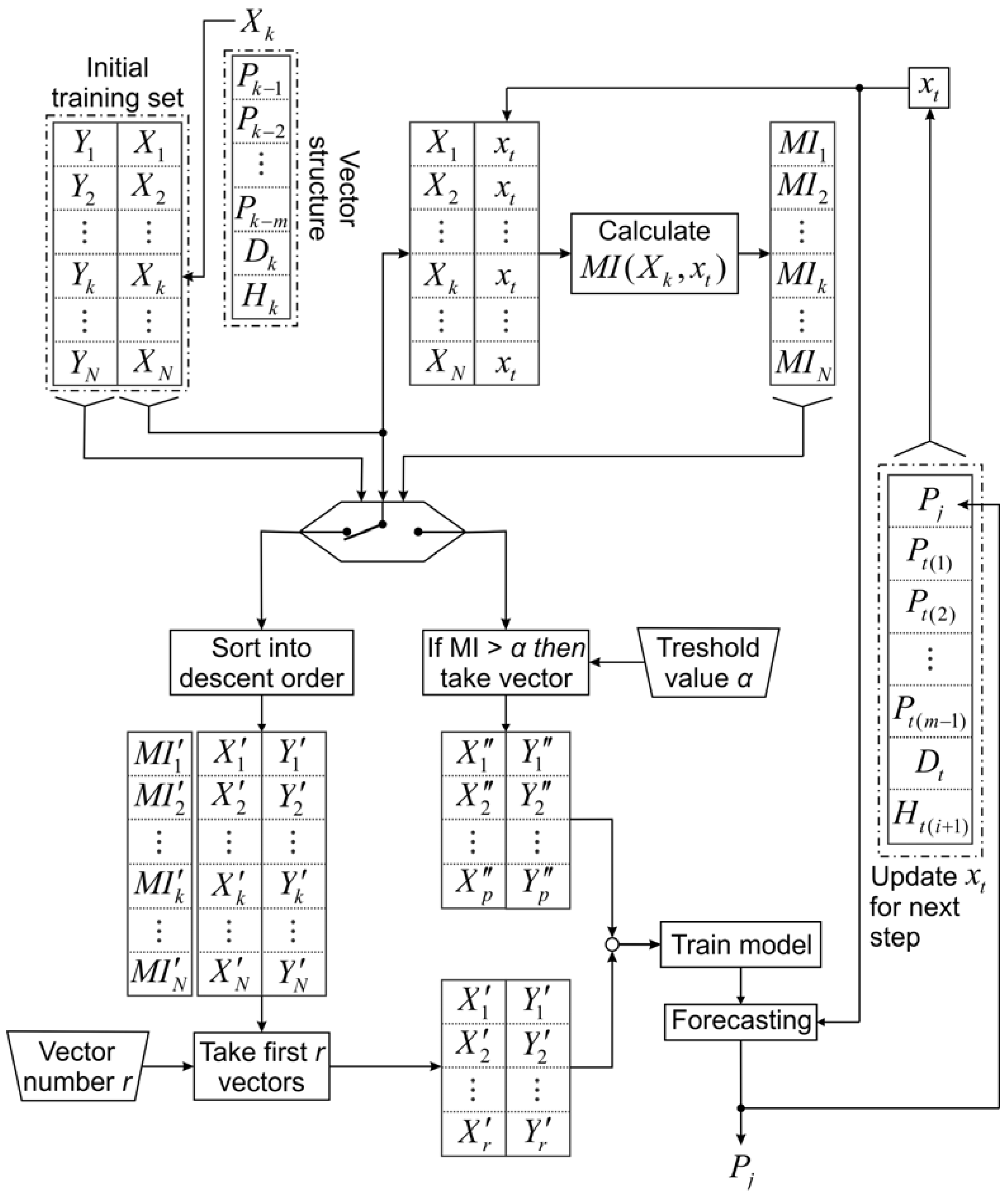
The structure of the input vectors can be seen in
Figure 4. Input vectors consist in total of
m+s features, where
m is the past load time-series features
Pi, i=1,..,24 and
s=2 non-time series features: the hour of the day
Hi,
and the day of the week
Di, where 1 corresponds to Monday, 2 to Tuesday and so on.
4. The Proposed Input Selection Algorithm and Forecasting Model
To achieve better model accuracy, the main goal before model training is to construct a new training set that fits the current forecasting scenario better. The idea behind this approach is to use some measurement criterion to recognize vectors from an initial training set which share the most information with the current forecasting scenario. While linear methods of analysis (like the correlation) can be useful, in general it is also essential to consider nonlinear relations between different variables. Because the mutual information measures arbitrary dependencies between random variables, it is suitable for assessing the “information content”, where methods based on linear relations in some cases may be prone to mistakes.
If
xk is the
kth training instance and
xt is the current forecasting instance, the MI between
xk and
xt is one criterion for measuring the dependence between them. In this way, by choosing instances which share a “greater” amount of MI with
xt, a greater prediction accuracy can be achieved by committing the model with input
xt. The proposed approach for instance selection according to the MI criterion is presented in Algorithm 1 and
Figure 4.
Let us first define the initial training set (X, Y), composed of N training vectors. The first step in the algorithm is the computation of MI between every instance in X and the current forecasting instance xt. Accordingly, the vector of MI values is established, which defines the significance of inputs in X versus xt. Two options are available for the selection of instances: the “MI threshold” or the “number of instances”.
Figure 4.
Architecture of the proposed inputs selection algorithm and forecasting strategy.
Figure 4.
Architecture of the proposed inputs selection algorithm and forecasting strategy.
When choosing the “MI threshold” as an option, parameter α must be provided. The predefined threshold value of α determines the sensitivity of the algorithm, i.e. the minimum degree of similarity allowed between the examined instance and xt, and needs to be set manually. All input vectors that have a greater amount of MI with xt and then α will be added to the new training set.
When the “number of inputs” is chosen as an option, the parameter r must be provided. The value of r defines the total number of instances that will be retained in the training set, and also needs to be set manually. First, the training set is sorted in descending order according to the values in the MI vector. Then the first r input vectors from the sorted initial training set are added into the new training set .
Algorithm 1. Instance selection according to MI.
- (1)
Initialization of the algorithm: from the available data, form the initial training and testing set, and choose one forecasting instance xt from the testing set.
- (2)
Calculate the MI between every vector from the initial training set xk k=1, ..., N and current forecasting instance xt, based on (3), and save these values in vector V(k).
- (3)
Reorder the initial training set in descending order according the values in
V vector. Then, based on
V vector and the resorted initial training set:
- a)
define a total number of vectors that will remain in the training set, denoted with r, or,
- b)
define the lower allowed limit bound for MI between initial training set vector and current forecasting instance xt, denoted with α.
- (4)
If the choice criterion is determined with α, based on vector V choose instances from the initial training set for which V(k) > α, k=1, ..., N holds and put them into a reduced training set .
- (5)
If the choice criterion is determined with r, form the reduced training set based on first r instances from the reordered initial training set.
- (6)
Train the LS-SVM model based on the reduced training set obtained from steps 4. or 5., apply it to current testing instance xt, obtain prediction, and then update xt for the next prediction step. Go to step 2. until predictions for all steps (hours of the current day) have been obtained.
- (7)
Choose another instance from the testing set xt and go to step 2. until predictions for all instances (daily loads by hours) in the training set have been obtained.
5. Experimental Results
For methodology evaluation, the forecasting of hourly loads from September 17 to September 30, 2011, was done for each day. The initial training set was formed by taking into account the calendar and weather congruence within the forecasting period. This is not necessary but it is obvious that using data for the model training from a similar calendar and weather period will give better forecasting accuracy. In this sense, the initial training set consists of the data for the month of September for the three previous years (2008, 2009 and 2010). The initial model is a recursive forecasting model generated with the initial training set. Three groups of models are generated with different training sets which are formed from the initial training set, each using different measurement criterion for input selection with an “MI threshold” or “number of inputs” option. Additionally, two models are generated with an initial training set, one based on simple average fitting and the other based on a recursive forecasting model with direct implementation. These models are denoted with:
- (1)
M0—a model trained with an initial training set that contains 2160 vectors,
- (2)
M1—a group of models trained with sets determined with a kNN MI criterion,
- (3)
M2—a group of models trained with sets determined with a kernel MI criterion,
- (4)
M3—a group of models trained with sets determined with a Pearson correlation coefficient criterion,
- (5)
M4—an average fit model, predictions are the average of the past 3 years of data based on day of the week and hour of the day congruence,
- (6)
M5—and the direct model, recursive forecasting model with direct implementation (without usage of forecasted values in future steps, but with true values instead).
Every model from M1–M3 is actually a group of models generated in each prediction step. To be precise, in each prediction step a new model is formed with the same feature set, but trained with a different training set which is prepared in accordance with the current prediction step. All models have the same structure, i.e. the feature set for every model M0–M5 is the same. Models M0, M4 and M5 are generated with the same initial training set, while models M1–M3 are generated with different training set which are formed from the initial training set in every prediction step, each using different measurement criterion for input selection with “MI threshold” or “number of inputs” selection option.
Error values shown in
Table 1 are in terms of Mean Absolute Percentage Error (MAPE) defined by:
where
and
are the real and the predicted value of the load demand in the
ith hour and
n is the number of hours. As seen from
Table 1, average, maximum and minimum daily MAPEs for the entire test set are given for each model. Models M1-M3 are based on input selection algorithm with the “MI threshold” or “number of inputs” selection option. For these models the results are obtained using both selection options, with “MI threshold” values: 0.5 and 0.6, 0.8 and 0.9, 0.98 and 0.99 for M1, M2 and M3 model respectively, denoted with TH
1 and TH
2. Likewise with “number of inputs” values: 50 and 100 for M1–M3 models, denoted with NI
1 and NI
2. The obtained results from
Table 1 indicate that model M1 has the best average MAPE over the entire test set in NI
1, TH
1 and TH
2 selecting scenarios while model M3 show the best results in the NI
2 scenario. To be precise, this is true if we disregard the results obtained with model M5 which gained the best results in general. However, it should be borne in mind that this model is not real because it uses true values in each prediction step which are not known in real situations.
Table 1.
Average, max and min daily MAPEs of the entire test set [%].
Table 1.
Average, max and min daily MAPEs of the entire test set [%].
| Model | M0 | M1 | M2 | M3 | M4 | M5 |
|---|
| | − | TH1 | TH2 | NI1 | NI2 | TH1 | TH2 | NI1 | NI2 | TH1 | TH2 | NI1 | NI2 | − | − |
| Avr. | 2.83 | 2.03 | 2.14 | 1.91 | 2.11 | 2.3 | 2.21 | 2.13 | 2.27 | 2.31 | 2.14 | 2.29 | 1.96 | 5.24 | 1.42 |
| Max | 4.64 | 4.09 | 4.9 | 3.65 | 4.08 | 5.65 | 4.96 | 5.55 | 5.53 | 3.31 | 5.27 | 5 | 4.28 | 7.95 | 2.72 |
| Min | 1.42 | 0.93 | 0.96 | 1 | 1.01 | 1.16 | 1.22 | 1.1 | 0.93 | 1.05 | 0.92 | 1.21 | 0.82 | 3.51 | 0.89 |
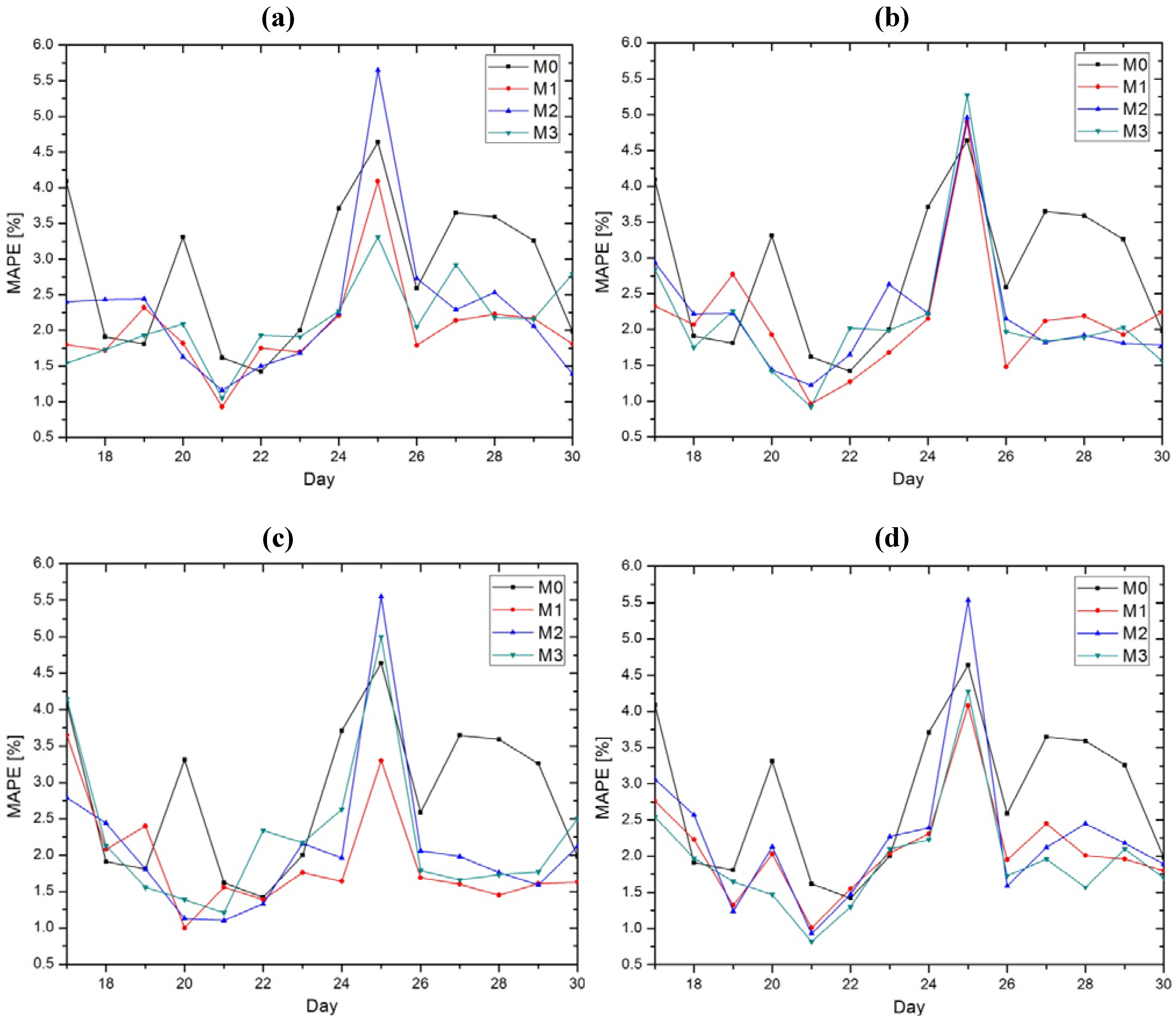
In order to gain a better insight, the average gaily MAPEs obtained by committing models with the test set are shown in
Figure 5. In this figure, a direct comparison in terms of MAPEs between the initial model M0, models with input selection M1–M3 and models without input selection M4 and M5, is given.
Figure 5 a, b, c and d show the results obtained with models M1–M3 using both selection options: the “MI threshold” and “number of inputs” option with two cases in both scenarios like in
Table 1.
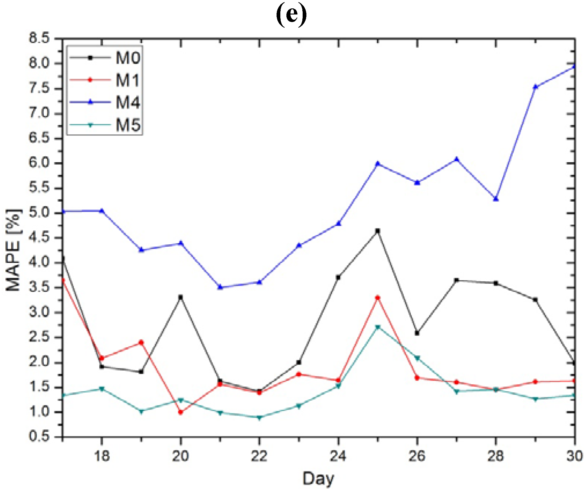
Figure 5e presents the results gained with models without the input selection option (M0, M4, M5) and model M1 for comparisons. In terms of MAPE, from
Table 1 and
Figure 5, it can be noted that the winning model is M1–NI
1 i.e., a model with input selection using
kNN MI estimator and “number of inputs” selection option with 50 input vectors for the training set. With the obtained results, the other models with input selection (M2 and M3) are close to model M1 and all these models with input selection outperform the initial model.
Beside the average daily MAPEs, from
Table 1 it can be noticed that model M1 reduces Max MAPEs in comparison to model M0 in three of the four cases, but also compared to models M2 and M3, which even increases Max MAPEs above 5% in some cases. Model M3 outperforms M1 only in one case in terms of Max MAPE. In respect of Min MAPEs, the situation is rather uniform even between models M1 and M3, which both have two winning entries. Nevertheless, model M1 outperforms models M0 and M2 in terms of Min MAPEs.
Figure 5.
Daily MAPEs for all of the generated models. (a) “MI threshold” selection option with 0.5 for M1, 0.8 for M2 and 0.98 for M3 (TH1), (b) “MI threshold” selection option with 0.6 for M1, 0.9 for M2 and 0.99 for M3 (TH2), (c) “number of inputs” selection option with 50 vectors for M1–M3 (NI1), (d) “number of inputs” selection option with 100 vectors for M1–M3 (NI2), (e) models without input selection with M1 for comparison.
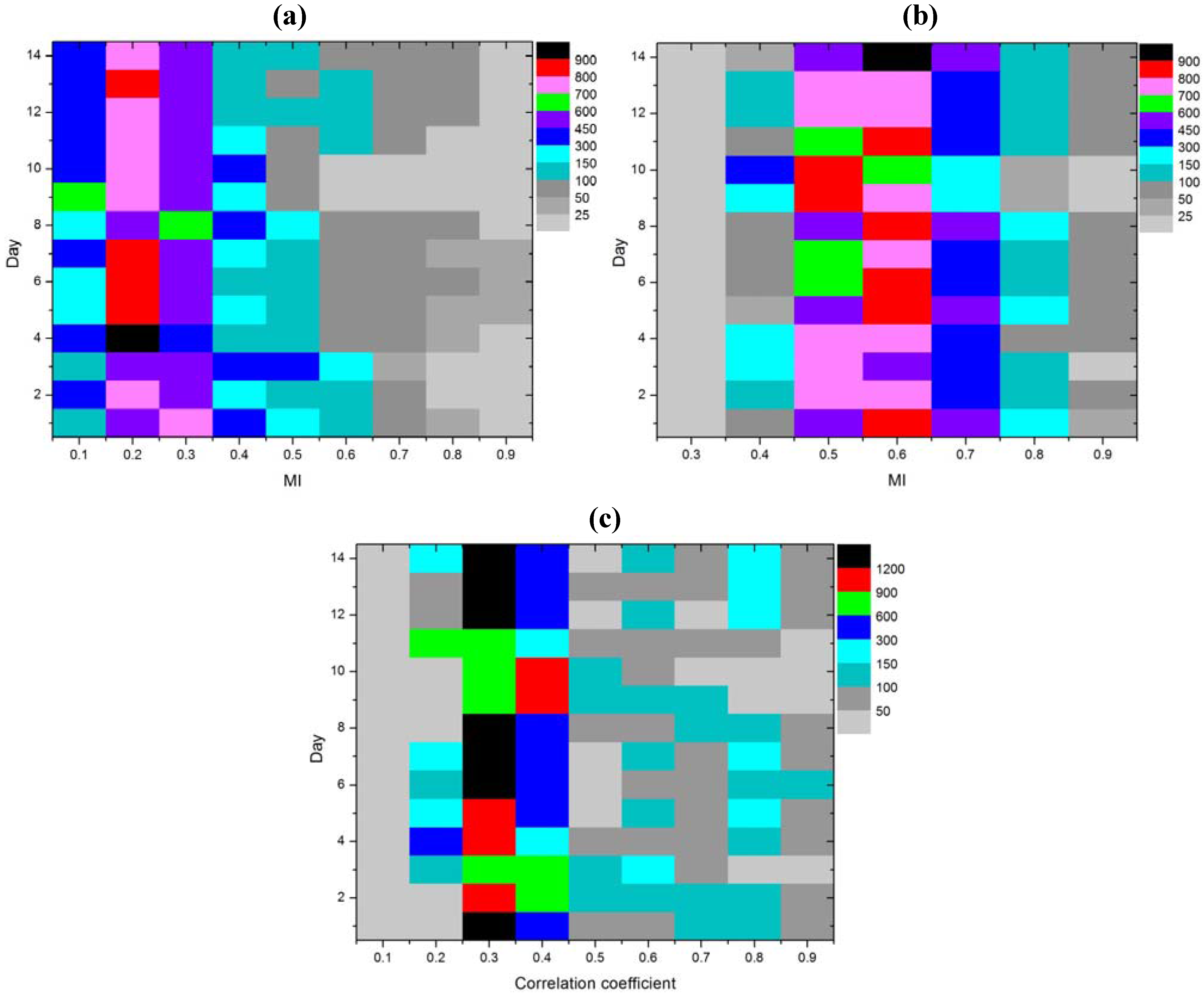
Vector number distribution in the initial training set, determined with a
kNN MI estimator, kernel MI estimator and correlation coefficient, for the first hour of each day, is shown in
Figure 6. On the horizontal axis we find the MI or Person correlation coefficient values, while the vertical axis represents the test day. Each field in
Figure 6 is represented by the appropriate color to match the number of vectors,
i.e., each color signifies a certain number of vectors. Thus, black blocks in the figure denote the number of vectors greater than 900 or 1200 and the opposite gray blocs mark the number of vectors smaller than 25 or 50.
As described in
Section 4, parameter
α determines the “MI threshold” which defines one selection option. In the experiments described in this section, the selected values for model M1 are
α = 0.5 and
α = 0.6 respectively, for model M2 are
α = 0.8 and
α = 0.9 and for model M3 are
α = 0.98 and
α = 0.99. To avoid any confusion, in the case of model M3, the “MI threshold” refers to the value of the Pearson correlation coefficient. As can be seen from
Figure 6, these are the values of MI or the correlation coefficient, for which an appropriate number of vectors to train a model were expected. It is appropriate in the sense that this number of vectors is sufficient for model training and on the other hand is not too large to load the model with unnecessary information. But as it turned out from
Table 1 and
Figure 5, the wining model uses a smaller number of training vectors which implies that the appropriate number of training vectors in this case is somewhere around 50.
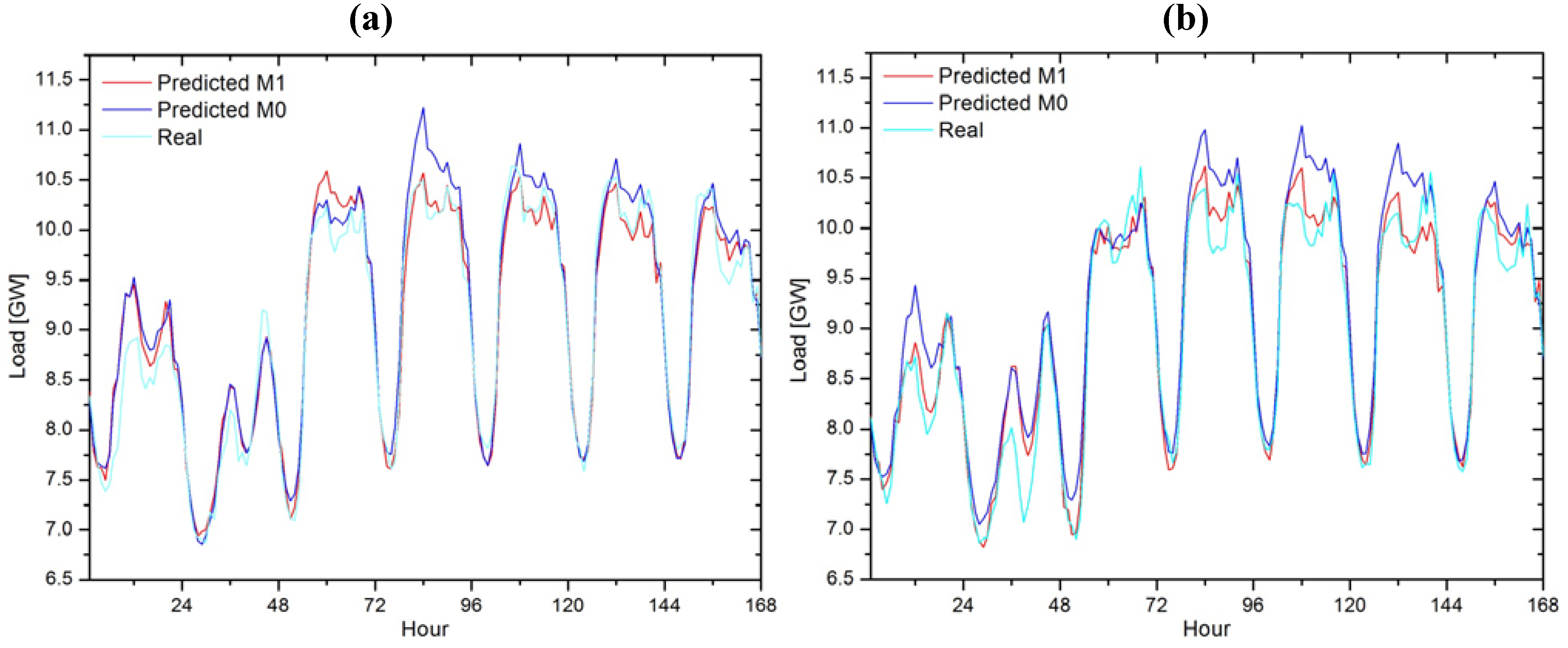
In
Figures 7, real and predicted hourly loads for two weeks in September are given, obtained from models M0 and M1. From these Figures it can be noticed that the predictions for model M1 have improved the shape and trend of the load curve in comparison to model M0. As seen from
Figure 5c, d and
Figure 7, the winning model behavior on day 19 is not like on the other predicted days. On this day, model M1 has a worse MAPE than the initial model, while model M2 has the best MAPE. In this situation the number of training vectors from model M1 is sufficient, but model M2, with a large number of vectors, gains better results.
Figure 6.
Vector number distribution in the initial training for the first hour of each day. (a) by kNN MI. (b) by kernel MI. (c) by correlation coefficient.
Figure 6.
Vector number distribution in the initial training for the first hour of each day. (a) by kNN MI. (b) by kernel MI. (c) by correlation coefficient.
Figure 7.
Real and predicted loads of models M0 and M1. (a) period from September 17 to 23, (b) period from September 24 to 30.
Figure 7.
Real and predicted loads of models M0 and M1. (a) period from September 17 to 23, (b) period from September 24 to 30.
The experiments were conducted on a computer with a Core i5 processor. The computational costs of the used algorithms are shown in
Table 2, where a comparison of the runtime is done in seconds. For each model three times are measured: one-step input selection time is an average runtime of input selection procedure in one forecasting step
i.e. this is the time of the calculation of the MI or Pearson correlation coefficient between one test vector and all the vectors in the initial training set and the selection of a new training set based on the selection criterion; one-step training time is an average runtime of model training on one forecasting step; total time is an average runtime of one day load forecasting
i.e. the total time needed to predict 24 hourly loads. The obtained results show that model M3 outperforms the others in terms of runtime, regardless of whether it is a case of input selection time, training time or total time. In addition, model M1 shows higher runtimes compared to models M2 and M3, as a result of the calculation need for
kNN MI estimation. However, the smaller runtimes of model M1 shows its advantage in comparison to the initial model M0.
Table 2.
Comparison of the runtime [s].
Table 2.
Comparison of the runtime [s].
| Model Time | M1 | M2 | M3 | M0 |
|---|
| One-step input selection time | 3.72 | 1.34 | 1.04 | - |
| One-step training time | 1.13 | 0.78 | 0.91 | 24.41 |
| Total time | 116 | 50.8 | 47 | 584 |
6. Conclusions
In this paper, a new load forecast strategy is proposed. The strategy is based on training set selection using the kNN based mutual information estimator in order to make an objective evaluation of how relevant an input vector is for the training set, i.e. how well it fits into the current prediction step.
Compared to other selection criteria, such as the kernel MI estimator and Pearson correlation coefficient, the kNN based MI estimator achieves better forecasting accuracy in most of the prediction scenarios, despite the fact that it has the longest selection time. As the experiment results present, improvements are especially evident in terms of reduction of average and max MAPEs.
In regard to other widely used methods that have dealt with input selection for STLF, such as similar day approaches and the clustering of load patterns, the proposed method is more general in terms of its ability to select appropriate inputs without the need for prior knowledge of the relationships between their features. Moreover, the presented method could be applied to various types of time-series prediction problems in addition to STLF.
As the experimental results have shown, all of the generated models which implement input selection strategy generally performed better than the initial model, despite the chosen input selection criterion, the kNN MI estimator, kernel MI estimator or Pearson correlation coefficient in combination with “number of inputs” or the “MI threshold” selection options. It has been shown that the quality of the training set is more significant than the size, that the models trained with sets of vectors which share a large amount of information with the forecasting input achieved greater accuracy than the models trained with a much larger set, chosen to fit the forecasting period.
Although the complexity of the calculations in the algorithms is quite robust, they bring significant improvements to load forecasting accuracy and could lead to an even more significant reduction in the time needed for models formation.
Furthermore, the development of a methodology for finding the optimum balance between the quality of the prediction and the size of the training sets for every prediction step can be the subject matter of future research.


