Nonstandard Approach to Gravity for the Dark Sector of the Universe

Abstract

We summarize the present state of research on the darkon fluid as a model for the dark sector of the Universe. Nonrelativistic massless particles are introduced as a realization of the Galilei group in an enlarged phase space. The additional degrees of freedom allow for a nonstandard, minimal coupling to gravity respecting Einstein’s equivalence principle. Extended to a self-gravitating fluid the Poisson equation for the gravitational potential contains a dynamically generated effective gravitational mass density of either sign. The equations of motion (EOMs) contain no free parameters and are invariant w.r.t. Milne gauge transformations. Fixing the gauge eliminates the unphysical degrees of freedom. The resulting Lagrangian possesses no free particle limit. The particles it describes, darkons, exist only as fluid particles of a self-gravitating fluid. This darkon fluid realizes the zero-mass Galilean algebra extended by dilations with dynamical exponent $z=\frac{5}{3}$. We reduce the EOMs to Friedmann-like equations and derive conserved quantities and a unique Hamiltonian dynamics by implementing dilation symmetry. By the Casimir of the Poisson-bracket (PB)-algebra we foliate the phase space and construct a Lagrangian in reduced phase space. We solve the Friedmann-like equations with the transition redshift and the value of the Casimir as integration constants. We obtain a deceleration phase for the early Universe and an acceleration phase for the late Universe in agreement with observations. Steady state equations in the spherically symmetric case may model a galactic halo. Numerical solutions of a nonlinear differential equation for the gravitational potential lead to predictions for the dark matter (DM) part of the rotation curves (RCs) of galaxies in qualitative agreement with observational data. We also present a general covariant generalization of the model.

1. Introduction

Understanding the dark sector of the Universe is one of the greatest challenges of today’s theoretical physics. The main question is whether the underlying astrophysical observations (missing gravitation in galactic systems resp. the accelerated expansion of the Universe) can be understood by means of known physical concepts, e.g., General Relativity (GR), or whether some kind of “new” physics is needed. Indeed, cosmic acceleration could be an apparent effect due to the averaging over large scale inhomogeneities in the Universe, but a reliable quantification of such an effect is not yet available (see the recent review [1]). On the other hand, there exists an overwhelming evidence for the existence of gravitational effects on all cosmological scales (termed “dark matter” (DM)), which cannot be explained by the gravitation of standard matter in the framework of GR (see the review [2]).

The current picture of cosmological structure formation assumes for DM some pressure less dust containing massive, perhaps weakly interacting cold particles (CDM). The present standard cosmological model (ΛCDM-model) uses besides CDM a positive cosmological constant Λ as the cause for the accelerated expansion of the Universe (see recent reviews on dark energy (DE), e.g., [3,4,5]). But, “favoured by a number of observations” [3], the ΛCDM-model suffers at least from the following insufficiencies:

• Interpreted as the energy density of the vacuum, the experimental value of Λ turns out to be a factor of about ${10}^{54}$ too small (see the recent estimate in [6]).
• None of the proposed CDM-constituents has been observed (cp. [7]).
• Rotation curves (RCs) of DM-dominated galaxies behave in their inner part in sharp contrast to the CDM-based simulations (known as the core-cusp problem [8]).

In a very recent paper, P. Kroupa [9] lists a large set of extragalactic observations that falsify the ΛCDM-model.

In this paper we will neither comment on the huge number of phenomenological models for a dynamical DE (see [3,4,5]), which all rest on at least one unknown function (e.g., a scalar field potential), nor comment on those modified gravity theories which explain DM-effects only (e.g., modified Newtonian dynamics (MOND) in its simplest, Milgromian form [10]). But we know of at least two kinds of modified gravity models which explain both, DE and DM i.e., the whole dark sector of the Universe:

• For MOND-models see Section 9 of the very recent review [11]. But all these models are very phenomenological in that they are based on one unknown “MOND function”.
• Modified theory of gravity (MOG) by Moffat [12] in which, besides the Einstein–Hilbert and matter actions, a massive vector field is introduced whose mass, coupling constant to matter and gravitational constant are promoted to scalar fields. The self-interaction potentials of these four fields are not fixed a priori and play the role of DE [13]. This model can explain galactic phenomena as e.g., RCs [14] as well as the accelerated expansion of the Universe and other cosmological observations [13].

In summary, all present attempts to explain quantitatively the new cosmological observations (e.g., late time cosmic acceleration) as well as the galactic RCs and other galactic phenomena contain either some new parameters or even free functions. If we assume that the cosmic acceleration is a real effect and not an apparent one (see above) then, obviously, we need some new (i.e., unconventional) physics which, however, should be based on known fundamental physical principles (e.g., symmetry).

In this paper we review some ongoing research on a model which is a first building block for a new theory describing the dark sector of the Universe. This model, introduced in [15] and further developed in [16,17], contains no new parameters in its Lagrangian and is based on well-known physical principles (Galilei symmetry and Einstein’s equivalence principle). The only free parameters appearing in our model are some integration constants (see Section 6 and Section 7). The basic idea it uses involves nonrelativistic massless particles. The use of such particles may appear very strange at a first sight as it seems to contradict Special Relativity according to which massless particles must move with the velocity of light. However, as we have shown before, we can introduce nonrelativistic massless particles if we enlarge the dimension of phase space; i.e., such particles are not described by position and momentum only. The additional degrees of freedom allow for a nonstandard, minimal coupling of these “exotic” particles [15] to gravity in accordance with Einstein’s equivalence principle. This coupling, for a self-gravitating fluid, leads to a dynamically generated effective gravitational mass density of either sign which is the source of the corresponding gravitational field. This fact leads to the possibility of using such a model as a first building block of a new theory describing the dark sector. In our approach we formulate the equivalence principle (local equivalence between gravitation and acceleration) as usual as an invariance of the dynamics w.r.t. arbitrary time-dependent translations (Milne gauge transformations). By fixing the gauge we can reduce the dimension of phase space and remove the unphysical variables. The Lagrangian of the resultant model does not possess a free particle limit and hence the particles it describes, called darkons, exist only as fluid particles of a self-gravitating fluid. This darkon fluid presents a dynamical realization of the zero-mass Galilean algebra extended by anisotropic dilations with the dynamical exponent $z=\frac{5}{3}$. This dilation symmetry emerges in a natural way from the minimal gravitational coupling. The cosmological EOMs are derived, as usual, from the darkon fluid EOMs by restricting the form of their solutions through the cosmological principle. However, the corresponding Hamiltonian cannot be derived from the darkon fluid Hamiltonian. So we have to derive a Hamiltonian and the corresponding Poisson-brackets (PBs) from the EOMs, a procedure which, as is well known, is not unique. So we construct, using the constants of motion, a Hamiltonian which has the correct scaling dimension and obtain the unique PBs by implementing the dilation symmetry. Moreover, our procedure allows us to construct a Lagrangian having foliated the phase space by means of the Casimir of the PB-algebra. We solve the cosmological EOMs and obtain, by fixing two integration constants by their values determined from experimental data, a prediction for the Hubble parameter $H(z)$ (z is the redshift) in general agreement with the existing data.

Furthermore, we demonstrate that our model not only gives a proper description of the late time cosmic acceleration but it also predicts galactic halos and, qualitatively correct, the corresponding flat rotation curves (RCs). To do this we derive for the spherically symmetric steady state case a nonlinear ordinary differential equation for the gravitational potential which is then solved numerically.

Almost all cosmological models are based on General Relativity (GR) or on some of its modifications which, however, preserve general covariance. The appearance of anisotropic dilations in our model seems, at first sight, to forbid a generalization of our model to a general covariant theory. But the dilation symmetry with $z=\frac{5}{3}$ is an emergent symmetry and not an input of our model. So we are able to propose a generalization of our model showing general covariance without imposing any form of scale symmetry.

One of the aims of the present paper is to show in detail the main ideas of our model. A comparison with observational data (Hubble parameter resp. galactic rotation curves) serves only as an illustration that it might be meaningful to develop the present model to a proper theory of gravitation for the dark sector of the Universe. For this reason we do not produce any least square fits for the undetermined integration constants appearing in the cosmological context.

The paper is organized as follows: In Section 2 we introduce Galilean massless particles and their coupling to gravity. In Section 3 we describe the generalization of this particle picture to a self-gravitating fluid, fix the gauge and so obtain the darkon fluid. Then, instead of the Poisson equation, we get a transport equation for the gravitational field. In Section 4 we describe the Hamiltonian dynamics of the darkon fluid to have a basis for quantization. Space-time symmetries of our model are discussed in Section 5. The darkon fluid cosmology is presented in Section 6. Starting with the cosmological principle we derive Friedmann-like equations, discuss the corresponding Hamiltonian dynamics and compare our predictions with the existing data for the Hubble diagram. In Section 7 we consider steady state equations in the spherically symmetric case and derive a nonlinear, ordinary differential equation (ODE) for the gravitational potential. Numerical solutions of this ODE lead to predictions for the behaviour of the DM-part of galactic RCs. In Section 8 we outline how to determine a correction to Newton’s gravitational law due to the cosmic expansion. Finally, in Section 9 we present a general covariant generalisation of our model. We close with some conclusions and give an outlook for future work.

2. Galilean Massless Particles and their Nonstandard Coupling to Gravity

As stated earlier, the introduction of nonrelativistic massless particles may appear very strange at first sight. It seems to contradict Special Relativity according to which massless particles must move with the velocity of light. But in Special Relativity, spinless particles are described by the vectors of position and momentum only. In our recent papers [15,16,17] we have shown that we can introduce nonrelativistic massless particles if we enlarge the dimension of the phase space from six to twelve. In subsection 2.1 we will show that this enlargement of phase space is also necessary: The 12-dimensional phase space is the minimal one allowing the dynamical realization of nonrelativistic massless particles.

How to couple gravity if there is no mass? Our nonrelativistic framework forbids the coupling to energy, as then this would be a relativistic effect. So we take Einstein${}^{\prime }$s equivalence principle as a starting point in subsection 2.2. Then, within the Lagrangian framework, the gravitational field will be coupled to one of the new degrees of freedom.

2.1. Galilean Massless Particles

Our first task involves finding a minimal dynamical realization of the unextended ($m=0$) Galilean algebra $G_0$ in three space dimensions.

$G_0$ is given by the Lie-brackets

$$[A_i,L_j]={ϵ}_{ijk}{A}_k,A_i\in (P_i,K_i,L_i)$$

$$[H,K_i]=P_i,[H,P_i]=[H,L_i]=0$$

(1)

$$[P_i,K_j]=0[P_i,P_j]=0,[K_i,K_j]=0$$

where $H,P_i,K_i$ and $L_i$ are the generators of time-resp. space translations, boosts and rotations.

A minimal dynamical realization of Equation (1) involves a construction of the elements of $G_0$ in terms of a minimal number of phase space variables and without the introduction of any free functions or parameters. Then the Lie-brackets in Equation (1) have to be understood as Poisson-brackets (PBs) w.r.t. the PB-algebra of phase space variables.

Let $\overrightarrow{x}(t)$ be a particle trajectory and $\overrightarrow{p}$ the corresponding conjugate momentum satisfying the fundamental PB-relation

$$[x_i,p_j]={\delta }_{ij}$$

(2)

The translation generator $\overrightarrow{P}$ acts on $\overrightarrow{x}$ resp. $\overrightarrow{p}$ as

$$[x_i,P_j]={\delta }_{ij}\text{resp}[p_i,P_j]=0$$

Therefore we get the identification

$$P_i=p_i.$$

(3)

To show that our minimally enlarged phase space contains, besides $\overrightarrow{x}$ and $\overrightarrow{p}$, two additional vectors corresponding to the reduced boost $\overrightarrow{q}$ and the velocity $\overrightarrow{y}$, we proceed in two steps:

• (1) Define a reduced boost vector $\overrightarrow{q}$

  $$q_i\equiv K_i-p_{i}t$$

  (4)
  The boost $\overrightarrow{K}$ acts on $\overrightarrow{x}$ as

  $$[x_i,K_j]={\delta }_{ij}t$$

  (5)
  leading by Equations (2) and (4) to

  $$[x_i,q_j]=0$$

  (6)
  Taking the PB of Equation (4) with $p_j$ it is easily seen by the expressions in Equation (1) that the PB of $p_i$ and $q_j$ vanishes

  $$[p_i,q_j]=0$$

  (7)
  Despite of Equations (6) and (7) $\overrightarrow{q}$ turns out to be nontrivial: Taking the PB of Equation (4) with H gives

  $${\dot{q}}_i=[q_i,H]=-p_i$$

  (8)
  Thus we conclude from Equations (6)–(8) that the $q_i$ are independent dynamical variables which, according to Equations (4) and (1), are commutative

  $$[q_i,q_j]=0$$

  (9)
• (2) Next we introduce the velocity vector

  $$y_i\equiv [x_i,H]$$

  (10)
  which is translationally invariant (take the PB of Equation (10) with $p_j$ and use the Jacobi identity) to get

  $$[y_i,p_j]=0$$

  (11)
  From Equations (10), (1), (2) and (5) we get the action of the boost generator on $y_i$

  $$[y_i,K_j]={\delta }_{ij}$$

  (12)
  Inserting now Equations (4) into (12) leads by Equation (11) to

  $$[y_i,q_j]={\delta }_{ij}$$

  (13)
  We conclude from Equations (13) and by (6), (7) and (9) that $\overrightarrow{y}$ cannot be a function of the other variables $\overrightarrow{x}$, $\overrightarrow{p}$ or $\overrightarrow{q}$.)
  To close the PB-algebra in phase space we choose, in accordance with the principle of a minimal dimension,

  $$[x_i,y_j]=0$$

  (14)
  Note that Equation (14) respects all Jacobi identities.

It remains to construct out of the phase space variables $\overrightarrow{x}$, $\overrightarrow{p}$, $\overrightarrow{q}$, and $\overrightarrow{y}$ the Hamiltonian H and the generator of rotations $\overrightarrow{L}$.

Our foregoing results lead to the EOMs

$${\dot{x}}_i=y_i,{\dot{p}}_i=0\text{and}{\dot{q}}_i=-p_i$$

(15)

but ${\dot{y}}_i$ has not yet been fixed.

The EOMs Equation (15) together with the canonical PBs

$$[x_i,p_j]={\delta }_{ij},[y_i,q_j]={\delta }_{ij}$$

(16)

imply that the Hamiltonian is given by

$$H=p_i{y}_i+f(\overrightarrow{q})$$

The principle of a minimal dynamical realization of $G_0$ forces us to put $f=0$. Thus we see that the Hamiltonian H is given by

$$H=p_i{y}_i$$

(17)

which leads, due to Equation (16), to the EOM for $y_i$, namely

$${\dot{y}}_i=0$$

(18)

The conserved generator of rotations $L_i$ is then given by

$$L_i={ϵ}_{ikl}(x_k{p}_l+y_k{q}_l)$$

(19)

The two parts of $L_i$ act separately on the $(\overrightarrow{x},\overrightarrow{p})$, resp. $(\overrightarrow{y},\overrightarrow{q})$ parts of the phase space.

The Hamiltonian dynamics given by H Equation (17) and the nonvanishing PBs Equation (16) is equivalent to the dynamics derived from the Lagrangian

$$L_0=p_i{\dot{x}}_i+q_i{\dot{y}}_i-p_i{y}_i$$

(20)

Finally we conclude

• A minimal dynamical realization of the unextended Galilei algebra in three dimensional configuration space requires a 12-dimensional phase space spanned by $(\overrightarrow{x},\overrightarrow{p},\overrightarrow{q},\overrightarrow{y})$
• The relation between energy H and the momenta (velocities) is nonstandard,
• Momenta $p_i$ and velocities $y_i$ are dynamically independent,
• The $q_i$ have no counterpart in standard particle mechanics,
• Galilean massless particles move with arbitrary finite velocity.

Dilations

$G_0$ may be enlarged by dilations with arbitrary dynamical exponent z. The corresponding generator has to satisfy the following PB-relations (cp [18] for $z=\frac{N}{2}$)

$$[D,H]=-H,[D,P_i]=-\frac{1}{z}{P}_i$$

(21)

$$[D,K_i]=\left(1-\frac{1}{z}\right)K_i,[D,L_i]=0$$

It can easily be checked that D is given by

$$D=tH-\frac{1}{z}{x}_i{p}_i+\left(1-\frac{1}{z}\right)y_i{q}_i$$

(22)

Below we will show that the value of z becomes fixed by the coupling of our massless particles to gravity.

2.2. Coupling to Gravity

To couple our massless particles to the gravitational field strength $g_i(\overrightarrow{x},t)$ we have to be consistent with Einstein${}^{\prime }$s equivalence principle: Locally, the gravitational field strength is equivalent to an accelerating frame. The only known nonrelativistic EOM for the particle trajectory satisfying this form of the equivalence principle is given by the Newton law:

$${\ddot{x}}_i(t)=g_i(\overrightarrow{x}(t),t)$$

(23)

because Equation (23) is invariant w.r.t. arbitrary time-dependent translations (Milne gauge transformations) [19]

$$x_i\to x_i^{{}^{\prime }}=x_i+a_i(t)$$

(24)

provided that $g_i$ transforms to

$$g_i^{{}^{\prime }}({\overrightarrow{x}}^{{}^{\prime }},t)=g_i(\overrightarrow{x},t)+{\ddot{a}}_i(t)$$

(25)

The EOM Equation (23) is realized if we add to $L_0$ an interaction part (minimal coupling)

$$L_{int}=-q_i{g}_i(\overrightarrow{x},t)$$

(26)

Then the EOM ${\ddot{q}}_i=0$ gets replaced by

$${\ddot{q}}_i=q_k{\partial }_i{g}_k$$

(27)

The total Lagrangian $L=L_0+L_{int}$ now becomes invariant w.r.t. the gauge transformations

$$x_i^{{}^{\prime }}=x_i+a_i(t),,y_i^{{}^{\prime }}=y_i+{\dot{a}}_i(t),p_i^{{}^{\prime }}=p_i,q_i^{{}^{\prime }}=q_i$$

(28)

$$g_i^{{}^{\prime }}({\overrightarrow{x}}^{{}^{\prime }},t)=g_i(\overrightarrow{x},t)+{\ddot{a}}_i(t)$$

This gauge invariance, resp. Einstein${}^{\prime }$s equivalence principle still holds if we add in Equation (26) further terms containing spatial derivatives of $g_i$ i.e., by replacing

$$g_i\to g_i-{\kappa }_1\Delta g_i+\text{higher}\text{order}\text{terms}$$

(29)

where Δ is the Laplacian and $K_1$ is a constant.

3. A Self-Gravitating (darkon) Fluid

3.1. Lagrangian formulation

In the last subsection (2.2) we have introduced a model for the motion of one Galilean massless particle in an external gravitational field $\overrightarrow{g}(\overrightarrow{x},t)$.

Now we want to generalize this model in two respects:

• (1) Instead of one particle we consider a continuum (fluid) labelled by comoving coordinates $\overrightarrow{\xi }\in {\mathbb{R}}^3$ (Lagrangian formulation of fluid dynamics, cp. [20]).
• (2) We treat the gravitational field $\overrightarrow{g}$ as a dynamical variable in order to get a self-gravitating fluid.

To realize the first point we substitute in the EOMs Equations (23) and (27)

$$x_i(t)\to x_i(\overrightarrow{\xi },t)\text{and}{q}_i(t)\to q_i(\overrightarrow{\xi },t)$$

(30)

To realize the second point we add to our previous Lagrangian $L_0+L_{int}$ a kinetic part $L_{field}$ for the gravitational field. We choose as usual

$$L_{field}=-\frac{1}{8\pi G}\int d^{3}x{(g_i(\overrightarrow{x},t))}^2$$

(31)

where G is Newton’s gravitational constant.

Then our Lagrangian, formulated in terms of $(x_i,{\dot{x}}_i),(q_i,{\dot{q}}_i)$ and $\overrightarrow{g}$, becomes

$$L=-n_0\int d^3\xi \left({\dot{q}}_i(\overrightarrow{\xi },t){\dot{x}}_i(\overrightarrow{\xi },t)+q_i(\overrightarrow{\xi },t)g_i(\overrightarrow{x}(\overrightarrow{\xi },t),t)\right)+L_{field}$$

(32)

where $n_0$ is the (constant) particle density in $\overrightarrow{\xi }$-space.

Varying $q_i$ , resp., $x_i$ leads to the continuum generalization of the previous EOMs Equations (23) and (27)

$${\ddot{x}}_i(\overrightarrow{\xi },t)=g_i(\overrightarrow{x}(\overrightarrow{\xi },t),t)$$

(33)

and

$${\ddot{q}}_i(\overrightarrow{\xi },t)=q_k(\overrightarrow{\xi },t)\frac{\partial }{\partial x_i}{g}_k(\overrightarrow{x}(\overrightarrow{\xi },t),t)$$

(34)

Now we have two possibilities to go further:

In the first case we take $g_i=-{\partial }_i\varphi$ and vary ϕ getting

$$\Delta \varphi =4\pi G{\partial }_k(n{q}_k)$$

(35)

with

$$n(\overrightarrow{x},t)=n_0{J}^{-1}{|}_{\overrightarrow{\xi }=\overrightarrow{\xi }(\overrightarrow{x},t)}\text{(particle}\text{density)}$$

(36)

and

$$J=det\left(\frac{\partial x_i(\overrightarrow{\xi },t)}{\partial {\xi }_k}\right)\text{(Jacobian)}$$

(37)

where $\overrightarrow{\xi }(\overrightarrow{x},t)$ denotes the function inverse to $\overrightarrow{x}(\overrightarrow{\xi },t)$.

The right hand side of the Poisson Equation (35) describes a dynamically generated effective gravitational mass density which may be of either sign with

• + sign leading to an attractive gravitation,
• - sign leading to a repulsive gravitation.

This promotes the self-gravitating fluid to being a possible candidate for the dark sector of the Universe. Note that our EOMs are invariant w.r.t the gauge transformations (see Equations (24) and (25))

$$x_i\to x_i+a_i(t)$$

(38)

when ϕ transforms as

$$\varphi (\overrightarrow{x},t)\to {\varphi }^{{}^{\prime }}({\overrightarrow{x}}^{{}^{\prime }},t)=\varphi (\overrightarrow{x},t)-{\ddot{a}}_i(t)x_i$$

(39)

and $q_i$ and n remain invariant.

In the second case we vary $g_i$ instead of ϕ and this leads to a linear relation between $q_i$ and $g_i$:

$$g_i(\overrightarrow{x},t)=-4\pi Gn(\overrightarrow{x},t)q_i(\overrightarrow{\xi }(\overrightarrow{x},t),t)$$

(40)

Note that the expression for $g_i$ can be rewritten as

$$q_i(\overrightarrow{\xi },t)=-\frac{1}{4\pi G}\left(\frac{g_i}{n}\right)(\overrightarrow{x}(\overrightarrow{\xi },t),t)$$

(41)

The expression (41) allows to eliminate, from the EOMs, the unphysical phase space variables $q_i$ in favour of the gravitational field strength $g_i$.

This removes the unphysical degrees of freedom. However, we have to pay a prize for this as now

• the gravitational field strength is not automatically given by the gradient of a potential,
• the expression (41) destroys the gauge symmetry i.e., it fixes the gauge.

Remark The gauge symmetry can be restored by considering a curl-free velocity field

$$\overrightarrow{u}=\overrightarrow{\nabla }u$$

and treating u as the variable to be varied [16].

Inserting $q_i$ from Equation (41) into the previous EOMs we get two coupled EOMs for $\overrightarrow{x}(\overrightarrow{\xi },t)$ and $\overrightarrow{g}(\overrightarrow{x}(\overrightarrow{\xi },t),t)$

$$\frac{d^2}{d{t}^2}{x}_i(\overrightarrow{\xi },t)=g_i(\overrightarrow{x}(\overrightarrow{\xi },t),t)$$

(42)

(initial condition $\overrightarrow{x}(\overrightarrow{\xi },0)=\overrightarrow{\xi }$) and

$$\frac{d^2}{d{t}^2}\left(\frac{g_i}{n}\right)=\frac{1}{2n}{\partial }_i{g}_k^2$$

(43)

Furthermore by inserting Equation (41) into the Lagrangian Equation (32) we obtain

$$L=\frac{n_0}{4\pi G}\int d^3\xi \frac{d}{dt}\left(\frac{g_i(\overrightarrow{x}(\overrightarrow{\xi },t),t)}{n}\right){\dot{x}}_i(\overrightarrow{\xi },t)+\frac{1}{8\pi G}\int d^{3}x{g}_i^2(\overrightarrow{x},t)$$

(44)

where we have used the identity

$$\int d^3\xi J{g}_i^2(\overrightarrow{x}(\overrightarrow{\xi },t),t)=\int d^{3}x{g}_i^2(\overrightarrow{x},t)$$

It can be easily checked that the Euler–Lagrange EOMs following from Equation (44) are identical with Equations (42) and (43).

The EOMs do not contain the gravitational constant G. The Lagrangian contains it only as a common factor. Moreover, our modified Lagrangian Equation (44) does not split into two parts involving a free and an interacting term. Clearly this strange property is a consequence of the phase space reduction due to Equation (41). We know only one other physical system possessing a similar property: the interacting Chaplygin gas if one eliminates the particle density from the Lagrangian (see [21], Section 2.1, item (i)).

3.2. Relabeling Symmetry and the Transport Equation for the Gravitational Field

Any fluid dynamics in the Lagrangian formulation has to be invariant under infinitesimal relabeling transformations (volume preserving diffeomorphisms) (see [20])

$$\overrightarrow{\xi }\to \overrightarrow{\xi }+\overrightarrow{\alpha }(\overrightarrow{\xi }),\text{with}\overrightarrow{\nabla }·\overrightarrow{\alpha }=0$$

(45)

For the corresponding Noether charge Q we obtain from the Lagrangian Equation (44)

$$Q=\int d^3\xi {\alpha }_i(\overrightarrow{\xi })\left(\frac{d}{dt}\left(\frac{g_k}{n}\right)\frac{\partial x_k}{\partial {\xi }_i}-\frac{g_k}{n}\frac{\partial {\dot{x}}_k}{\partial {\xi }_i}\right)$$

(46)

where we have already performed one partial integration. But from the EOMs Equations (42) and (43) it follows that the integrand in Equation (46) is already conserved i.e., that

$${\theta }_i\equiv \frac{\partial {\dot{x}}_k}{\partial {\xi }_i}\frac{g_k}{n}-\frac{\partial x_k}{\partial {\xi }_i}\frac{d}{dt}\left(\frac{g_k}{n}\right)$$

(47)

is a conserved quantity and so is a function of $\overrightarrow{\xi }$ only. By solving Equation (47) for $\frac{d}{dt}\left(\frac{g_k}{n}\right)$ we obtain the once-integrated form of the EOM Equation (43)

$$\frac{d}{dt}\left(\frac{g_i}{n}\right)=\frac{g_k}{n}\frac{\partial {\dot{x}}_k}{\partial x_i}-{\theta }_k(\overrightarrow{\xi })\frac{\partial {\xi }_k}{\partial x_i}$$

(48)

which is a transport equation for the gravitational field (cf. [22] for the standard self-gravitating dust fluid).

3.3. Eulerian Formulation

In the Lagrangian formulation the fluid particles are labelled by comoving coordinates $\overrightarrow{\xi }$. So a Lagrangian observer moves with the particle. On the other hand an Eulerian observer is located at a fixed position $\overrightarrow{x}$ (see [20]). Therefore we obtain the fluid fields in the Eulerian formulation from the ones given in the Lagrangian formulation by the following change of independent variables

$$(\overrightarrow{\xi },t)\to (\overrightarrow{x},t)\text{with}\overrightarrow{x}=\overrightarrow{x}(\overrightarrow{\xi },t)$$

(49)

Correspondingly, we have to transform the time derivatives

$$\frac{d}{dt}\to D_t=\frac{\partial }{\partial t}+u_k(\overrightarrow{x},t)\frac{\partial }{\partial x_k}\text{(convective}\text{derivative)}$$

(50)

with

$$u_k(\overrightarrow{x},t)\equiv \frac{d}{dt}{x}_k(\overrightarrow{\xi },t){|}_{\overrightarrow{\xi }=\overrightarrow{\xi }(\overrightarrow{x},t)}$$

(51)

The EOMs then become:

Euler Equation

$$D_t{u}_i=g_i$$

(52)

Transport Equation for the gravitational field:

$$D_t\left(\frac{g_i}{n}\right)=\frac{g_k}{n}{\partial }_i{u}_k-{\theta }_i$$

(53)

where the auxiliary variable

$${\theta }_i(\overrightarrow{x},t)\equiv \frac{\partial {\xi }_k}{\partial x_i}{\theta }_k(\overrightarrow{\xi }){|}_{\overrightarrow{\xi }=\overrightarrow{\xi }(\overrightarrow{x},t)}$$

obeys the EOM

$$D_t{\theta }_i+{\theta }_k{\partial }_i{u}_k=0$$

(54)

and the particle density n obeys the continuity Equation:

$${\partial }_{t}n+{\partial }_k(n{u}_k)=0$$

(55)

All these equations can be derived from the Lagrangian

$$L=-\frac{1}{4\pi G}\int d^{3}x\left(g_i(D_t{u}_i-\frac{1}{2}{g}_i)+\theta ({\partial }_{t}n+{\partial }_k(n{u}_k))-n\alpha D_t\beta \right)$$

(56)

Here θ, α and β give the Clebsch-parameterization of the vector field ${\theta }_i(\overrightarrow{x},t)$

$${\theta }_i={\partial }_i\theta +\alpha {\partial }_i\beta$$

(57)

They obey the Euler–Lagrange EOMs

$$D_t\theta =D_t\alpha =D_t\beta =0$$

(58)

Operating with $D_t$ on Equation (57) leads then to the EOM Equation (54) for ${\theta }_i$. All the remaining EOMs are Euler–Lagrange EOMs derived from Equation (56).

3.4. Coupling with Baryonic Matter

We describe baryonic matter (B) by a standard self-gravitating fluid coupled to the darkon fluid by the jointly created gravitational field ϕ. Then, within the Lagrangian formulation, we have to add to Equation (32) the following baryonic Lagrangian

$$L_B=m\int d^3\xi \left(\frac{{({\dot{x}}_i^B(\overrightarrow{\xi },t))}^2}{2}-\varphi ({\overrightarrow{x}}^B(\overrightarrow{\xi },t))\right)$$

(59)

where m is the (constant) baryonic mass density in $\overrightarrow{\xi }$ -space.

Varying $x_i^B$ leads to the Newton equation

$${\ddot{x}}_i^B(\overrightarrow{\xi },t)=-{\partial }_i\varphi ({\overrightarrow{x}}^B(\overrightarrow{\xi },t),t)$$

(60)

whereas varying ϕ in the total Lagrangian

$$L=L_D+L_B+L_{field}$$

(61)

where $L_D$ is the darkon fluid Lagrangian (first term in Equation (34)), leads to the Poisson Equation

$$\nabla \varphi =4\pi G\left({\partial }_k(n{q}_k)+{\rho }_B\right)$$

(62)

whose r.h.s. consists of the sum of the darkon fluid source and the usual B-source. The B-mass density ${\rho }_B$ is defined by

$${\rho }_B(\overrightarrow{x},t)=m{J}^{-1}{|}_{\overrightarrow{\xi }=\overrightarrow{\xi }(\overrightarrow{x},t)}$$

(63)

where J is the Jacobian defined by Equation (37). We note that ${\rho }_B$ satisfies the local conservation law (continuity Equation)

$${\partial }_t{\rho }_B+{\partial }_k(u_k^B{\rho }_B)=0$$

(64)

where ${\overrightarrow{u}}^B$ is defined analogously to Equation (51).

Adding baryonic matter leads to the following changes in the foregoing subsections: The gravitational force appearing in $L_D$ is the total one $g_i=-{\partial }_i\varphi$ and so is it in the case of the EOMs Equations (33) and (34). The solution of the Poisson Equation (62) is a superposition of the gravitational potentials created by the B and the D-sources

$$\varphi ={\varphi }_B+{\varphi }_D$$

(65)

with

$$\Delta {\varphi }_B=4\pi G{\rho }_B$$

(66)

and

$${\partial }_k{\varphi }_D=4\pi Gn{q}_k$$

(67)

So Equation (67) is now the substitute for Equation (41) and, therefore, the conserved quantity Equation (47) becomes (note that $L_B$ is separately invariant w.r.t. relabeling transformations Equation (45))

$${\theta }_i=-\frac{\partial {\dot{x}}_k}{\partial {\xi }_i}\frac{{\partial }_k{\varphi }_D}{n}+\frac{\partial x_k}{\partial {\xi }_i}\frac{d}{dt}\left(\frac{{\partial }_k{\varphi }_D}{n}\right)$$

(68)

Then, in the Eulerian formulation, we obtain finally instead of Equation (53) the transport equation

$$D_t\left(\frac{{\partial }_i{\varphi }_D}{n}\right)=\frac{{\partial }_k{\varphi }_D}{n}{\partial }_i{u}_k+{\theta }_i$$

(69)

where ${\theta }_i$ obeys the EOM Equation (54).

4. Hamiltonian Dynamics

The derivation of the Hamiltonian dynamics, ie the formulation of classical dynamics in terms of a Hamiltonian and a PB-algebra, is an indispensable prerequisite for any quantization procedure. We start with the Lagrangian Equation (56) from which we obtain immediately the Hamiltonian

$$H=\frac{1}{4\pi G}\int d^{3}x\left(g_i(u_k{\partial }_k{u}_i-\frac{1}{2}{g}_i)-n{\theta }_i{u}_i\right)$$

(70)

where we have used the identity [21]

$$\theta {\partial }_k(n{u}_k)-n{u}_k\alpha {\partial }_k\beta =-n{\theta }_k{u}_k+{\partial }_k(u_{k}n\theta )$$

(71)

and then neglected the boundary contribution arising from the last term in Equation (71). For the Hamiltonian EOM

$$\dot{A}(\overrightarrow{x},t)=[A(\overrightarrow{x},t),H]$$

(72)

we choose as independent field variables $A\in (n,\theta ,n\alpha ,\beta ,u_i,g_i)$. To read off from Equations (70) and (72) the PBs for the A-fields we next rewrite their EOM as follows:

$$\dot{n}=-{\partial }_k(u_{k}n),\dot{\theta }=-u_k{\partial }_k\theta$$

$${(n\alpha )}^{·}=-{\partial }_k(u_{k}n\alpha ),\dot{\beta }=-u_k{\partial }_k\beta$$

$${\dot{u}}_i=-u_k{\partial }_k{u}_i+g_i\text{and}$$

(73)

$${\dot{g}}_i=g_k{\partial }_i{u}_k-{\partial }_k(u_k{g}_i)-n{\theta }_i$$

where

$${\theta }_i={\partial }_i\theta +\alpha {\partial }_i\beta$$

The EOM (73) have the Hamiltonian form Equation (72) if the fluid fields A obey the following nonvanishing PBs

$$[\theta (\overrightarrow{x},t),n({\overrightarrow{x}}^{{}^{\prime }},t)]=4\pi G\delta (\overrightarrow{x}-{\overrightarrow{x}}^{{}^{\prime }})$$

(74)

$$[\beta (\overrightarrow{x},t),(n\alpha )({\overrightarrow{x}}^{{}^{\prime }},t)]=4\pi G\delta (\overrightarrow{x}-{\overrightarrow{x}}^{{}^{\prime }})$$

(75)

and

$$[g_i(\overrightarrow{x},t),u_j({\overrightarrow{x}}^{{}^{\prime }},t)]=4\pi G{\delta }_{ij}\delta (\overrightarrow{x}-{\overrightarrow{x}}^{{}^{\prime }})$$

(76)

For these PBs all Jacobi identities are trivially fulfilled. It is interesting to note that the PB-algebra Equations (74)–(76) decomposes into three irreducible parts. Each component has a canonical structure which allows quantization by applying Dirac${}^{\prime }$s rule (details will be given in a separate paper)

$${[A,B]}_{PB}\to \frac{1}{i\hslash }[\widehat{A},\widehat{B}]$$

(77)

where $\widehat{A}(\widehat{B})$ denotes the quantum operator corresponding to the classical function $A(B)$ . The PB-algebra Equations (74)–(76) possesses a Casimir (being a quantity whose PBs with all elements of the PB-algebra vanish) defined by

$$C\equiv \int d^{3}x{ϵ}_{ikl}\frac{\partial {\theta }_l(\overrightarrow{x},t)}{\partial x_k}{\theta }_i(\overrightarrow{x},t)$$

(78)

To prove that C is a Casimir we proceed in two steps:

• We choose a particular relabeling transformation Equation (45) with ${\alpha }_i(\overrightarrow{\xi })=-{ϵ}_{ikl}\frac{\partial {\theta }_l(\overrightarrow{\xi })}{\partial {\xi }_k}$. The corresponding Noether charge Equation (46) is then given by

  $$Q=\int d^3\xi {ϵ}_{ikl}\frac{\partial {\theta }_l(\overrightarrow{\xi })}{\partial {\xi }_k}{\theta }_i(\overrightarrow{\xi })$$

  (79)

  But Eulerian variables do not respond to a relabeling of the Lagrange variable $\overrightarrow{\xi }$ [21]. So Q is a Casimir of the PB-algebra Equations (74)–(76).
• It remains to express Q in terms of Eulerian variables. To do this, we get from the definition of ${\theta }_i(\overrightarrow{x},t)$

  $${\theta }_i(\overrightarrow{\xi })={\theta }_k(\overrightarrow{x}(\overrightarrow{\xi },t),t)\frac{\partial x_k}{\partial {\xi }_i}$$

  (80)

  However, using Equation (80) and the identity

  $${ϵ}_{ikl}\frac{\partial x_n}{\partial {\xi }_l}\frac{\partial x_m}{\partial {\xi }_i}=J{ϵ}_{nmj}\frac{\partial {\xi }_k}{\partial x_j}$$

  (81)

  we obtain

  $${ϵ}_{ikl}\frac{\partial {\theta }_l(\overrightarrow{\xi })}{\partial {\xi }_k}{\theta }_i(\overrightarrow{\xi })=J{ϵ}_{mjn}\frac{\partial {\theta }_m(\overrightarrow{x},t)}{\partial x_j}{\theta }_m(\overrightarrow{x},t){|}_{\overrightarrow{x}=\overrightarrow{x}(\overrightarrow{\xi },t)}$$

  Hence we finally have

  $$Q=C$$

  (82)

Of course the Casimir property of C can be shown also directly by bracketing Equation (78) with all fluid fields and using the PB-algebra Equations (74)–(76).

We recall that C vanishes if ${\theta }_i(\overrightarrow{x},t)$ is given by the Clebsch parametrization Equation (57) with non-singular functions $\theta ,\alpha ,\beta$ vanishing at infinity [21].

We note that the vortex helicity

$$H_e\equiv \int d^{3}x\overrightarrow{u}(\overrightarrow{x},t)·\overrightarrow{\omega }(\overrightarrow{x},t)$$

(83)

where

$$\overrightarrow{\omega }\equiv \overrightarrow{\nabla }\times \overrightarrow{u}$$

which is a Casimir in standard fluid dynamics, is not a Casimir in the case of our model. $H_e$ is a conserved quantity if $\overrightarrow{g}$ is the gradient of a potential, but it has a non-trivial PB with $\overrightarrow{g}$, namely:

$$[g_i(\overrightarrow{x},t),H_e]=8\pi G{\omega }_i(\overrightarrow{x},t)$$

(84)

Up to now we have used, within the Hamiltonian framework, those fluid fields which lead to the simplest possible form Equations (74)–(76) for the PB-algebra. But in many applications it is more convenient to introduce instead of the auxiliary field ${\theta }_i$ the momentum field $p_i$

$$4\pi G{p}_i(\overrightarrow{x},t)=D_t\left(\frac{g_i}{n}\right)=\frac{g_k}{n}{\partial }_i{u}_k-{\theta }_i$$

(85)

where we have used the definition of $p_i$ in the Lagrangian formulation

$$p_i(\overrightarrow{\xi },t)\equiv -{\dot{q}}_i(\overrightarrow{\xi },t)=\frac{1}{4\pi G}\frac{d}{dt}\left(\frac{g_i}{n}\right){|}_{\overrightarrow{x}=\overrightarrow{x}(\overrightarrow{\xi },t)}$$

and then changed to the Eulerian formulation. In terms of the momentum density $n{p}_i$ we obtain for our PB-algebra, besides the PB-relation Equation (76),

$$[(n{p}_i)(\overrightarrow{x},t),n({\overrightarrow{x}}^{{}^{\prime }},t)]=-n(\overrightarrow{x},t){\partial }_i\delta (\overrightarrow{x}-{\overrightarrow{x}}^{{}^{\prime }})$$

(86)

$$[(n{p}_i)(\overrightarrow{x},t),u_k({\overrightarrow{x}}^{{}^{\prime }},t)]={\partial }_i{u}_k\delta (\overrightarrow{x}-{\overrightarrow{x}}^{{}^{\prime }})$$

(87)

$$[(n{p}_i)(\overrightarrow{x},t),g_k({\overrightarrow{x}}^{{}^{\prime }},t)]=-g_k(\overrightarrow{x},t){\partial }_i\delta (\overrightarrow{x}-{\overrightarrow{x}}^{{}^{\prime }})$$

(88)

$$[(n{p}_i)(\overrightarrow{x},t),(n{p}_j)({\overrightarrow{x}}^{{}^{\prime }},t)]=-(n{p}_j)(\overrightarrow{x},t){\partial }_i\delta (\overrightarrow{x}-{\overrightarrow{x}}^{{}^{\prime }})+(n{p}_i)({\overrightarrow{x}}^{{}^{\prime }},t){\partial }_j^{\prime }\delta (\overrightarrow{x}-{\overrightarrow{x}}^{{}^{\prime }})$$

(89)

which can be obtained from the transformation formulae

$$n(\overrightarrow{x},t)=\int d^3\xi \delta (\overrightarrow{x}-\overrightarrow{x}(\overrightarrow{\xi },t))$$

(90)

$$(nA)(\overrightarrow{x},t)=\int d^3\xi A(\overrightarrow{\xi },t)\delta (\overrightarrow{x}-\overrightarrow{x}(\overrightarrow{\xi },t)),A\in (p_i,u_i,g_i)$$

(91)

and the canonical PBs in the Lagrange formulation (continuum generalization of Equation (16))

$$[x_i(\overrightarrow{\xi },t),p_j({\overrightarrow{\xi }}^{{}^{\prime }},t)]={\delta }_{ij}\delta (\overrightarrow{\xi }-{\overrightarrow{\xi }}^{{}^{\prime }})$$

(92)

and

$$[{\dot{x}}_i(\overrightarrow{\xi },t),q_j({\overrightarrow{\xi }}^{{}^{\prime }},t)]={\delta }_{ij}\delta (\overrightarrow{\xi }-{\overrightarrow{\xi }}^{{}^{\prime }})$$

(93)

if, in addition, we use the relation Equation (41) for $g_j$.

5. Space-time Symmetries

In this section we will show

• The darkon fluid possesses the unextended (zero mass) Galilei algebra $G_0$ as a symmetry algebra. The corresponding energy-momentum tensor is not symmetric and contains a negative pressure term.
• $G_0$ may be enlarged by dilations with dynamical exponent $z=\frac{5}{3}$. This particular value of z is determined by the minimal coupling to gravity as given by Equation (26).
• Expansions are not a symmetry of the darkon fluid.

5.1. Space-time Translations and the Energy-momentum Tensor

The linear momentum (generator of space translations) is given by

$$P_i=\int d^{3}x(n{p}_i)(\overrightarrow{x},t)$$

(94)

where the momentum density $n{p}_i$ obeys the local conservation law

$${\partial }_t(n{p}_i)=-{\partial }_k(u_{k}n{p}_i)+\frac{1}{8\pi G}{\partial }_i{g}_k^2=-{\partial }_k{T}_{ik}$$

(95)

Thus the momentum tensor

$$T_{ik}=n{p}_i{u}_k+\mathcal{P}{\delta }_{ik}\text{with}\mathcal{P}=-\frac{1}{8\pi G}{g}_k^2$$

(96)

is not symmetric and the pressure $\mathcal{P}$ is negative.

The Hamiltonian Equation (70) (generator of time translations), expressed in terms of the momentum density, takes the form

$$H=\int d^{3}x{T}_{tt}(\overrightarrow{x},t)$$

(97)

with

$$T_{tt}=n{u}_i{p}_i-\frac{1}{8\pi G}{g}_i^2$$

(98)

The energy density $T_{tt}$, of course, obeys the local conservation law

$${\partial }_t{T}_{tt}=-{\partial }_k{T}_{tk}$$

(99)

with

$$T_{tk}=u_k\left(T_{tt}+\mathcal{P}\right)$$

If we identify, as usual, the space-time component of the energy-momentum tensor with the momentum density

$$T_{it}=n{p}_i$$

(100)

we may conclude, that the energy-momentum tensor $T_{\alpha ,\beta }$ with $\alpha ,\beta \in (t,k)$ obeys the standard conservation law

$${\partial }_t{T}_{\beta ,t}+{\partial }_k{T}_{\beta ,k}=0$$

(101)

But, because $T_{\alpha \beta }$ is not symmetric, we note that

$${\partial }_t{T}_{t\beta }+{\partial }_k{T}_{k\beta }\ne 0$$

(102)

We remark that such a nonsymmetric energy-momentum tensor was introduced for the first time in 1947 by Weyssenhoff and Raabe [23].

5.2. Zero mass Galilean Symmetry

Galilean boosts are generated by

$$K_i=t{P}_i-\frac{1}{4\pi G}\int d^{3}x{g}_i$$

(103)

which is a conserved quantity because the EOM for the gravitational field $g_i$ is given, due to Equations (73) and (85), by

$${\dot{g}}_i=n{p}_i-{\partial }_k(u_k{g}_i)$$

(104)

The PB of the boost generator $K_i$ and the momentum $P_j$ vanishes

$$[K_i,P_j]=0$$

(105)

as is easily see from the fact that $P_i$ is the generator of space translations

$$[P_i,A(\overrightarrow{x},t)]={\partial }_{i}A(\overrightarrow{x},t)\text{for}\text{any}A.$$

(106)

The vanishing of the right hand side of Equation (105) tells us that the total mass of the darkon fluid is zero.

5.3. Angular Momentum

The continuum generalization of expression Equation (19) for the one-particle angular momentum is given by

$$L_i={ϵ}_{ikl}{n}_0\int d^3\xi (x_k(\overrightarrow{\xi },t)p_l(\overrightarrow{\xi },t)+{\dot{x}}_k(\overrightarrow{\xi },t)q_l(\overrightarrow{\xi },t))$$

(107)

By using the identity Equation (41) and by passing to the Eulerian variables we obtain

$$L_i={ϵ}_{ikl}\int d^{3}x\left(x_{k}n{p}_l-\frac{1}{4\pi G}{u}_k{g}_l\right).$$

(108)

5.4. Anisotropic Scaling

Anisotropic scaling, characterized by a dynamical exponent $z\ne 1$, implies that the time and space variables transform differently w.r.t. dilations

$$t\to t^{*}=\lambda t,\overrightarrow{x}\to {\overrightarrow{x}}^{*}={\lambda }^{\frac{1}{z}}\overrightarrow{x},\text{with}\lambda >0$$

(109)

In Section 2.1 we have shown that the dynamics of free massless particles allows for an implementation of dilations with an arbitrary z. To see what happens in the case of a darkon fluid we consider a continuum generalization of Equation (22) of the generator of dilations D

$$D=tH-\frac{1}{z}\int d^{3}xn{p}_i{x}_i-\frac{(1-\frac{1}{z})}{4\pi G}\int d^{3}x{u}_i{g}_i$$

(110)

where in the last term we have used the relation Equation (41) between the field $\overrightarrow{q}$ and the gravitational field $\overrightarrow{g}$. Taking now the time derivative of D Equation (110) and by using the EOMs Equation (73) we obtain

$$\frac{d}{dt}D=\frac{1}{8\pi G}\left(-3+\frac{5}{z}\right)\int d^{3}x{g}_i^2$$

(111)

Thus D is conserved if z takes the value $z=\frac{5}{3}$. It may easily be checked that with $z=\frac{5}{3}$ all PBs between D and the elements of $G_0$ are in agreement with the PB-relations Equation (21).

The dilations are implemented by the following transformation of the fluid fields A

$$A(\overrightarrow{x},t)\to A^{*}(\overrightarrow{x},t)={\lambda }^{\frac{z_A}{z}}A({\overrightarrow{x}}^{*},t^{*})$$

(112)

where $z_A$ denotes the scale dimension of A. . For an infinitesimal dilation we get

$$[A(\overrightarrow{x},t),D]=\left(t{\partial }_t+\frac{1}{z}(x_k{\partial }_k+z_A)\right)A(\overrightarrow{x},t)$$

(113)

which leads, due to the explicit form of D Equation (110) and the PBs Equations (76), (86)–(88), to the following values for the $z_A$:

$$z_n=3,z_{{\theta }_i}=1,z_{g_i}=\frac{7}{3},z_{u_i}=\frac{2}{3}$$

(114)

and therefore, due to Equation (85), $z_{p_i}=1.$

Let us finally prove that our EOMs are not invariant with respect to expansions. We prove this by demonstrating the contradiction. So consider the expansions:

$$t\to t^{*}=\Omega (t)t,\overrightarrow{x}\to {\overrightarrow{x}}^{*}=\Omega {(t)}^{\frac{2}{z}}\overrightarrow{x}\text{with}\Omega (t)=\frac{1}{1-\kappa t}$$

(115)

Suppose that we would be able to implement such expansions. Then there would exist a generator K of expansions, which obeys, in combination with H and D, an $O(2,1)$ algebra. On the other hand, as is well known [18], the PB-algebra between the elements of $G_0$ and the $O(2,1)$ algebra would not close for $z\ne 2$. The PB between K and the generator of boosts $K_i$ would then imply the existence of a conserved generator of accelerations $F_i$

$$[K,K_i]=\left(1-\frac{2}{z}\right)F_i$$

(116)

But we know from the discussion given in Section 3 that the relation Equation (41) between the field $\overrightarrow{q}$ and the gravitational field $\overrightarrow{g}$ destroys the invariance of our EOMs w.r.t. arbitrary time dependent translations (gauge transformations), in particular w.r.t. to constant accelerations. This contradicts the initial supposition of the existence of expansions as a symmetry of the EOMs.

Note that the coupling of our darkon fluid to baryonic matter (see 3.4) will break dilation symmetry.

6. Darkon Fluid Cosmology

We consider the darkon fluid as a model for the dark sector of the Universe. Hence we look for solutions of the fluid EOMs satisfying the cosmological principle (the Universe is supposed to be isotropic and homogeneous on large scales). The relevant cosmological EOMs are listed in subsection 6.1. In subsection 6.2 we derive and discuss the corresponding Hamiltonian dynamics. We start with the three cosmological EOMs in 1st-order form, derive the two constants of motion and construct out of them that Hamiltonian which has the correct scaling dimension. Unique expressions for the corresponding PBs are obtained if we consider explicitly the implementation of dilation symmetry. For that purpose it is convenient to introduce new independent variables with either scale dimension zero or one. The PB-algebra possesses one Casimir which can be used to obtain a foliation of the three-dimensional phase space into an infinite number of two-dimensional phase spaces. Within the two-dimensional phase space we get a completely integrable system. We are able to construct a corresponding Lagrangian.

Due to the appearance of a constraint it is not possible to quantize the arising Hamiltonian by applying the Dirac quantization rule. An alternative way seems to be the affine quantization (see [24]).

In subsection 6.3 we solve the cosmological EOMs with the cosmological redshift z as the independent variable. By choosing some integration constants to be positive our model shows qualitatively the transition from a deceleration to an acceleration phase of the Universe. Fixing two integration constants by observational values we obtain a prediction for the cosmological history in general agreement with the existing data of the Hubble parameter.

6.1. Cosmological EOMs

The realization of the cosmological principle within the Lagrangian formulation leads to the following structure for the field variables

$$x_i(\overrightarrow{\xi },t)=a(t){\xi }_i$$

(117)

$$n(\overrightarrow{x},t)=n(t)$$

(118)

where $a(t)$ is the cosmological scale factor, and

$$g_i(\overrightarrow{x},t)=\frac{n(t)}{n_0}g(a(t))x_i,n_0=n(0)$$

(119)

The split of the r.h.s. of Equation (119) into two factors and defining g as a function of $a(t)$ are a matter of convenience. If we next put all this into the original EOMs we obtain the following cosmological EOMs

• From the definition of n (see Equation (36)) we get

  $$n(t)=\frac{n_0}{a^3(t)}$$

  (120)
• From the EOM Equation (42) and using Equation (120) we get

  $$\ddot{a}(t)=\frac{g(a)}{a^2(t)}$$

  (121)

  which is a Friedmann-like equation.
• From the EOM for $g_i$ Equation (43) and the definition of ${\theta }_i$ (see Equation (47)) we get

  $$\dot{g}(a(t))=\frac{K_1}{a^2(t)},K_1=\text{const.}$$

  (122)

  where $K_1$ is related to ${\theta }_i$ by

$${\theta }_i(\overrightarrow{\xi })=-\frac{K_1}{n_0}{\xi }_i$$

(123)

We note that possible derivative terms in the gravitational coupling Equation (29) give no contribution to the cosmological EOMs. Taking into account, additionally, baryonic matter (see 3.4) will not change the cosmological EOMs. In such a case $g(a)$ would be changed by an additive constant (see [15]).

6.2. Hamiltonian Dynamics

The cosmological EOMs Equations (121) and (122), when written in 1st-order form, take the form

$$\dot{a}=b,\dot{b}=\frac{g}{a^2},\dot{g}=\frac{K_1}{a^2}$$

(124)

So we have to consider a dynamical system in a three-dimensional space. This finite dimensional space, called usually mini-superspace, will be the phase space for our Hamiltonian dynamics. The dynamical system Equation (124) possesses two constants of motion

$$Q_2=b{K}_1-\frac{g^2}{2}$$

(125)

and

$$Q_3=\frac{g^3}{6}+Q_{2}g+\frac{K_1^2}{a}$$

(126)

In order to construct Hamiltonian dynamics for the dynamical system Equation (124) we have to find a Hamiltonian H and the Poisson-brackets (PBs) $[x_{\alpha },x_{\beta }]$ for $x_{\alpha }\in (a,b,g)$ such, that the EOMs Equation (124) become the Hamiltonian EOMs

$${\dot{x}}_{\alpha }=[x_{\alpha },H]\equiv f_{\alpha }$$

(127)

where the PBs are required to fulfill the Jacobi-identities and H has to be a function of the two constants of motion $Q_2$ and $Q_3$ only. To reduce the arbitrariness in the construction of H we note that the EOMs Equation (124) are dilation invariant, i.e., if $x_{\alpha }$ are solutions of Equation (124) then, by the transformation $x_{\alpha }\to x_{\alpha }^{\star }$

$$x_{\alpha }^{\star }(t)={\lambda }^{z_{\alpha }}{x}_{\alpha }(\lambda t),\lambda >0$$

(128)

with $z_a=-\frac{3}{5}$, $z_b=\frac{2}{5}$, $z_g=\frac{1}{5}$ we obtain another set of solutions. For the scaling exponents of the constants of motion we obtain

$$z_{Q_2}=\frac{2}{5},\text{and}{z}_{Q_3}=\frac{3}{5}$$

(129)

Let D be the conserved generator of dilations. Then we get from Equations (127) and (128) that

$$[x_{\alpha },D]=f_{\alpha }t+z_{\alpha }{x}_{\alpha }\equiv {\eta }_{\alpha }$$

(130)

(with no summation over α in the middle term!) leading to

$$D=Ht-f,\text{with}\dot{f}=H$$

(131)

which is equivalent to

$$[H,D]=H$$

(132)

However, this expression tells us that we have $z_H=1.$ Thus neither $Q_2$ nor $Q_3$ but $Q_2{Q}_3$ is a possible candidate for the Hamiltonian H. So we choose

$$H=\frac{Q_2{Q}_3}{K_1^3}$$

(133)

where the factor $K_1^{-3}$ has been inserted in order to get a simple form for H which will be obtained when we rewrite it in terms of some new variables, which will be introduced below. With this H the PBs for the $x_{\alpha }$ have, according to Equation (127), to be chosen such, that

$$[x_{\alpha },x_{\beta }]\frac{\partial H}{\partial x_{\beta }}=f_{\alpha }$$

(134)

holds. But Equation (134) is equivalent to

$$A_{\alpha \beta }{y}_{\beta }=f_{\alpha }$$

(135)

where

$$y_{\beta }\equiv \frac{1}{2}{ϵ}_{\beta \gamma \delta }[x_{\gamma },x_{\delta }]\text{and}{A}_{\beta \alpha }\equiv -{ϵ}_{\beta \alpha \gamma }\frac{\partial H}{\partial x_{\gamma }}$$

(136)

The matrix $A_{\alpha \beta }$ is not invertible (it is anti-symmetric and of odd order). Therefore Equation (135) has no unique solution for the variables $y_{\beta }$. Even if we require in addition, the validity of the Jacobi identities, the solutions for the $y_{\beta }$ will not be unique. To render the PBs unique we must consider also the implementation of the dilation symmetry. First of all Equations (130) and (131) may be rewritten as

$$[f,x_{\alpha }]=z_{\alpha }{x}_{\alpha }$$

(137)

and

$$[f,D]=Ht$$

(138)

From Equation (138) we conclude that $z_f=0$ . Thus f is a function of the dilation invariant variables $x=\frac{a{g}^3}{K_1^2}$ and $y=\frac{b{K}_1}{g^2}$ only. Then from $z_x=z_y=0$ and Equation (137) we obtain

$$0=[f,x]=[y,x]\frac{\partial f}{\partial y}$$

and

$$0=[f,y]=[x,y]\frac{\partial f}{\partial x}$$

which shows that the PB between x and y has to vanish

$$[x,y]=0$$

(139)

As the third variable (of our phase space) besides x and y we choose $w=\frac{g^2}{a{K}_1}$ which has $z_w=1$. Then, due to $z_H=1$ the Hamiltonian H Equation (133) has the structure

$$H=wh(x,y)$$

(140)

with

$$h(x,y)=\left(y-\frac{1}{2}\right)\left(1+x\left(y-\frac{1}{3}\right)\right)$$

(141)

In order to determine the remaining PBs $[x,w]$ and $[y,w]$ we next rewrite the EOMs Equation (124) in terms of the new variables x, y and w

$$\dot{x}=w(xy+3),\dot{y}=-\frac{2w}{x}\left(y-\frac{1}{2}\right)\text{and}\dot{w}=w^2\left(\frac{2}{x}-y\right)$$

(142)

But Equation (142) are required to be EOMs derivable from the Hamiltonian H. So we get with Equation (140)

$$[x,H]=[x,w]h=w(xy+3)\text{and}[y,H]=[y,w]h=-\frac{2w}{x}\left(y-\frac{1}{2}\right)$$

(143)

Solving Equation (143) for the two PBs gives us

$$[x,w]=\frac{w(xy+3)}{h},[y,w]=-\frac{2w(y-\frac{1}{2})}{xh}$$

(144)

It is easy to check that the PBs Equations (139) and (144) satisfy all Jacobi identities.

Expressing now the original variables a, b and g in terms of x, y and w

$$a=K_1^{\frac{1}{5}}{(xw)}^{-\frac{3}{5}}x,b=K_1^{\frac{1}{5}}{(xw)}^{\frac{2}{5}}y,g=K_1^{\frac{3}{5}}{(xw)}^{\frac{1}{5}}$$

(145)

we obtain their PBs

$$[a,b]=H^{-1}\left(\frac{2}{5}{b}^2+\frac{3}{5}\frac{g}{a}\right),[a,g]=H^{-1}\left(\frac{bg}{5}+\frac{3}{5}\frac{K_1}{a}\right)$$

(146)

and

$$[b,g]=-\frac{2}{5}\frac{K_1^3}{a^2{Q}_3}$$

The Equation (146) can be summarized by one equation

$$[x_{\alpha },x_{\beta }]=H^{-1}(f_{\alpha }{z}_{\beta }{x}_{\beta }-f_{\beta }{z}_{\alpha }{x}_{\alpha })$$

(147)

(no summation over α or β.) The PB-algebra Equation (147) is identical with a construction given by Hojman [25] who starts also with some EOMs, a Hamiltonian and a symmetry. But in contrast to [25] our derivation of Equation (147) shows for the particular case of dilation symmetry the uniqueness of the PB-algebra.

6.2.1. One Exact Solution

The EOMs Equation (142) have a simple power law solution of the form

$$x(t)=-6,y(t)=\frac{1}{2},\frac{1}{w(t)}=\frac{5}{6}(t-t_0)$$

(148)

which for $t_0=0$ are dilation invariant. We will later show that Equation (148) governs the behaviour of the cosmological solutions at early times. Furthermore the solution Equation (148) determines a relative minimum of the Hamiltonian Equation (140) at $H=0$.

6.2.2. Reduced Phase Space

In the following we will solve the EOMs Equation (142) for x as a function of y. So we reduce the dimension of phase space from three to two. To do that we can either use standard analytical methods or algebraic methods. The latter shows more clearly the physical nature of this reduction. For this reason we will present both methods.

Analytical method

From the first two EOMs in Equation (142) we obtain immediately an ODE of Bernoulli type for $x(y)$

$$x^{{}^{\prime }}(y)=\frac{x(xy+3)}{1-2y}$$

(149)

where $x^{{}^{\prime }}(y)\equiv \frac{dx(y)}{dy}$ . As usual we use the transformation

$$x(y)\to u(y)\equiv \frac{1}{x(y)}$$

(150)

to obtain a linear ODE for $u(y)$

$$u^{{}^{\prime }}(y)+\frac{3u(y)}{1-2y}+\frac{y}{1-2y}=0$$

(151)

The point $y=\frac{1}{2}$ is a singular point of the DE Equation (151).Therefore we obtain one solution $u_{-}(y)$ for $y<\frac{1}{2}$ and another one $u_{+}(y)$ for $y>\frac{1}{2}$.

$$u_{-}(y)=\frac{1}{3}-y+k_{-}{\left(\frac{1}{2}-y\right)}^{\frac{3}{2}},u_{+}(y)=\frac{1}{3}-y+k_{+}{\left(y-\frac{1}{2}\right)}^{\frac{3}{2}}$$

(152)

with real-valued constants $k_{+}$ and $k_{-}$. Note that the first term in Equation (152) represents a particular solution of the inhomogeneous DE Equation (151) whereas the second one represents the most general solution of the homogeneous part. The two solutions $u_{\pm }$ are not connected to each other by an analytical continuation in y. This implies that the reduced phase space consists of two dynamically disconnected parts with either $y<\frac{1}{2}$ or with $y>\frac{1}{2}$ . We will show later that the validity of the condition

$$y>\frac{1}{2}$$

(153)

is necessary in order to explain the accelerating expansion of the Universe. So we will use $y>\frac{1}{2}$ exclusively in the following.

Algebraic method

The PB-algebra Equations (139) and (144) possesses a Casimir

$$C=Q_3{Q}_2^{-\frac{3}{2}}$$

(154)

where we have used the equivalence between Equation (153) and the condition

$$Q_2>0$$

(155)

To prove the Casimir-property of C we observe first that $z_C=0$. So C can depend only on x and y. By using the definition of the $Q_i$, $i=2,3$ and the transformation formula Equation (145) we obtain

$$C={(y-\frac{1}{2})}^{-\frac{3}{2}}\left(\frac{1}{x}+y-\frac{1}{3}\right)$$

(156)

Therefore, due to Equation (139), the PBs $[x,C]$ and $[y,C]$ both vanish. To show that $[w,C]=0$ too we use Equation (139) again by considering the chain of relations

$$0=[H,C]=[w,C]\frac{\partial H}{\partial w}$$

(157)

But as $\frac{\partial H}{\partial w}\ne 0$ we see that $[w,C]$ must vanish.

This reasoning shows that any function of the independent variables which is a constant of motion and has a vanishing scaling exponent is a Casimir of our PB-algebra. But there exists no other function, functionally independent from Equation (154), which possesses this property. Now we use the fact that the equation

$$C(x,y)=k,k\in {\mathbb{R}}^1$$

(158)

defines, for different values of k, a foliation of the three-dimensional phase space (cp [26]). So we may solve Equation (154) for x at fixed k and obtain

$$x(k,y)=\frac{1}{\frac{1}{3}-y+k{(y-\frac{1}{2})}^{\frac{3}{2}}},y>\frac{1}{2}$$

(159)

in accordance with Equation (152) if we identify $k=k_{+}$.

This way we see that our system is described by a Hamiltonian dynamics on a two-dimensional phase space with variables w and y and the Hamiltonian

$$H=w\left(y-\frac{1}{2}\right)\left(1+x(k,y)\left(y-\frac{1}{3}\right)\right)=kwx(k,y){\left(y-\frac{1}{2}\right)}^{\frac{5}{2}}$$

(160)

where for the last equality we have used Equation (159), and the PB

$$[w,y]=\frac{2w}{k{x}^2(k,y)(y-\frac{1}{2}{)}^{\frac{3}{2}}}$$

(161)

leading together to the following Hamiltonian EOM

$$\dot{y}=-\frac{2w}{x(k,y)}\left(y-\frac{1}{2}\right),\dot{w}=w^2\left(\frac{2}{x(k,y)}-y\right)$$

(162)

The dynamical system Equation (162) is completely integrable. To show this we make use of the existence of a second constant of motion besides the Casimir (see Equations (125) and (126)). In this proof we may use the Hamiltonian H (160). Let us put $H=E$, E=const. Then we can solve Equation (160) for w

$$w(E,k,y)=\frac{E}{kx(k,y){(y-\frac{1}{2})}^{\frac{5}{2}}}$$

(163)

Inserting Equation (163) into the first Equation in (162) we finally obtain $y(t)$ by a quadrature.

Generator of dilations

We can also give an explicit expression for the generator of dilations in two-dimensional phase space. From $\dot{f}=H$ Equation (131) we get $\dot{y}\frac{\partial f}{\partial y}=H$ and so

$$\frac{\partial f}{\partial y}=-\frac{k}{2}{x}^2(k,y){\left(y-\frac{1}{2}\right)}^{\frac{3}{2}}\equiv F(y)$$

(164)

Lagrangian

The EOMs Equation (162) are Euler–Lagrange EOM derived from the Lagrangian

$$L=\dot{y}F(y)logw-H(w,y)$$

(165)

where $H(w,y)$ is given by Equation (160). To prove this it is sufficient to note that

$$\Pi (y,w)\equiv F(y)logw$$

(166)

is the momentum canonically conjugate to y. Indeed, by using Equation (161) we obtain

$$[y,\Pi (y,w)]=1$$

(167)

We can now use Equation (166) to eliminate w from the Hamiltonian Equation (160) to obtain

$$H=kx(k,y){\left(y-\frac{1}{2}\right)}^{\frac{5}{2}}exp\left(\frac{\Pi }{F(y)}\right)$$

(168)

With Equations (167) and (168) we have finally Hamiltonian dynamics in a two-dimensional phase space expressed in terms of canonical variables y and Π.

How to quantize this system?

We would like to quantize the system Equations (167) and (168) with the constraint Equation (153). This cannot be done if we try to follow Dirac${}^{\prime }$s rule of going from the classical PB Equation (167) to the quantum commutator

$$[\widehat{y},\widehat{\Pi }]=i\hslash$$

(169)

The reason for this is that, for self-adjoint operators $\widehat{y}$ and $\widehat{\Pi }$ Equation (169) has, up to unitary equivalence, only one irreducible representation given by $\widehat{\Pi }=\frac{\hslash }{i}\frac{\partial }{\partial y}$ ($-\infty <y<\infty )$ (cp [24]). So the spectrum of $\widehat{y}$ covers the whole real axis. To overcome this difficulty we follow J. Klauder (see [24]) and consider instead of the canonical quantization Equation (169) the affine quantization given by

$$[\widehat{q},\widehat{D}]=i\hslash \widehat{q}$$

with $q\equiv y-\frac{1}{2}$ and

$$\widehat{D}\equiv \frac{1}{2}(\widehat{\Pi }\widehat{q}+\widehat{q}\widehat{\Pi })$$

(170)

and choose the irreducible representation for $q>0$. Details of such a quantization procedure still have to be worked out.

6.3. Solution of the EOMs

Let us first put the two constants of motion $Q_{2,3}$ equal to numbers $K_{2,3}$. Next we solve the defining equation of $K_2$ Equation (125) for $\dot{a}=b$ and obtain

$$\dot{a}=\frac{1}{K_1}\left(K_2+\frac{g^2}{2}\right)$$

(171)

So, with $K_2>0$, equivalent to condition Equation (153), we must have

$$K_1>0$$

(172)

in order to describe an expanding Universe.

Using the definition of $K_3$ Equation (126) we obtain (we consider now g as a function of the redshift z, ${(1+z)}^{-1}\equiv a$), a cubic equation for $g(z)$:

$$\frac{g^3}{6}+K_{2}g=K_3\left(1-\frac{1+z}{1+z_t}\right)$$

(173)

where the transition redshift $z_t$ is defined by

$$\frac{1}{1+z_t}=\frac{K_1^2}{K_3}.$$

(174)

Let us look now at Equation (173) for $K_2>0$ and $K_3>0$ together with the Friedmann-like equation (see Equation (121))

$$\ddot{a}=g(z){(1+z)}^2$$

(175)

For $z>z_t$ we have $g<0$ and so, due to Equation (175) $\ddot{a}<0$. So, for $z>z_t$ we are in the deceleration phase of the early Universe. On the other hand, for $z<z_t$ we have $g>0$ and then, due to Equation (175), $\ddot{a}>0$. So, for $z<z_t$ we are in the acceleration phase of the late Universe. To get these results we have to require that $K_{2,3}>0$.

To see this note that

• From Equation (174) we conclude that $K_3>0$.
• Let $z_t$ be a zero of g. Then differentiating Equation (173) at $z=z_t$ shows that $\frac{K_2}{K_3}{g}^{{}^{\prime }}(z_t)<0$. But the transition from the decelerating to the accelerating phase requires $g^{{}^{\prime }}(z_t)<0$. . Thus we must have $\frac{K_2}{K_3}>0$.

Next, to simplify Equation (173) we introduce

$$\tilde{g}(z)=K_2^{-\frac{1}{2}}g(z)$$

(176)

Then Equation (173) becomes (we recall that $k=K_3{K}_2^{-\frac{3}{2}}$)

$$\frac{{\tilde{g}}^3}{6}+\tilde{g}=k\left(1-\frac{1+z}{1+z_t}\right)$$

(177)

where $\tilde{g}$ now depends on the two parameters $z_t$ and k only.

Using Equation (171) the Hubble parameter $H(z)\equiv \frac{\dot{a}}{a}(z)$ may be expressed in terms of $\tilde{g}$

$$H(z)=\frac{K_2}{K_1}\left(1+\frac{{\tilde{g}}^2(z)}{2}\right)(1+z)$$

(178)

However, it is more convenient to consider instead of $H(z)$ the normalized Hubble parameter

$$h(z)=\frac{H(z)}{H_0}$$

(179)

for which we find

$$h(z)=\frac{(1+z)\left(1+\frac{{\tilde{g}}^2(z)}{2}\right)}{\left(1+\frac{{\tilde{g}}^2(0)}{2}\right)}$$

(180)

So, if we know $H_0$, the cosmological history is determined in our model completely by the two parameters $z_t$ and k.

To obtain k in terms of observable quantities we consider the deceleration parameter

$$q(z)=-\frac{\ddot{a}}{a{H}^2}=\frac{h^{{}^{\prime }}(z)}{h(z)}(1+z)-1$$

(181)

which, when expressed in terms of $\tilde{g}$, $z_t$ and k takes the form:

$$q(z)=-\frac{k(1+z)}{1+z_t}\tilde{g}(z){\left(1+\frac{{\tilde{g}}^2(z)}{2}\right)}^{-2}$$

(182)

Thus the value of k can be determined from the knowledge of the present deceleration parameter $q_0=q(0)$ and of $z_t$.

Remark: The expressions for $\tilde{g}(z)$, $h(z)$ and $q(z)$ in our paper [15] can be obtained from the present ones by the substitutions $\tilde{g}(z)\to -\sqrt{6}\tilde{g}(z)$ and $k\to \sqrt{6}k$. Furthermore, the constants $K_1$ and $n_0$ are related to the constants D and β from [15] by the relations $K_1=-3D\beta$ and $n_0=\frac{3D}{4\pi }.$

Asymptotic results for $z\gg z_t$

From Equation (177) we obtain

$$\tilde{g}(z)\sim -{\left(6k\frac{z}{1+z_t}\right)}^{\frac{1}{3}}$$

(183)

Thus we obtain a power law behaviour for $h(z)$

$$h(z)\propto z^{\frac{5}{3}}$$

(184)

which shows that asymptotically our cosmological solutions are scale invariant. On the other hand the deceleration parameter reaches asymptotically a constant value

$$q(z)\sim \frac{2}{3}.$$

(185)

The asymptotic behaviour Equation (184) differs from the predictions of the ΛCDM-model

$$h_{\Lambda CDM}(z)\sim z^{\frac{3}{2}}$$

(186)

for the matter dominated epoch. But we expect a change of our prediction Equation (184) if we generalise our model to the one that exhibits general covariance (cp. Section 9).

6.4. Distances

We must decide how to relate observational data of distances (e.g., of supernovae) to the Hubble parameter $H(z)$. In standard FLRW cosmology we obtain, in terms of comoving coordinates for a flat Universe and for a radial light ray (see Section 1.2 in [27]) the coordinate distance

$$\xi (z)=c{\int }_0^z\frac{d{z}^{\prime }}{H(z^{\prime })}$$

(187)

In any relativistic theory of gravitation which possesses a metric the limit of an isotropic, homogeneous and flat Universe is described by the FLRW metric given in comoving coordinates by

$$d{s}^2=a^2(t){(d\overrightarrow{\xi })}^2-c^2{(dt)}^2$$

(188)

Then Equation (187) arises from the requirement that light propagates along a null geodesic

$$ds=0$$

(189)

Note that our darkon fluid model is neither a relativistic nor a metric theory. However, it may be understood as a limiting case of such a theory as shown in Section 9. On the other hand, in a nonrelativistic theory we do not have an expanding space but only moving particles in a static space. But both points of view lead to the same observable effects as has been already noted by Milne in 1934 [19]. We need only to assume “that, relative to a particular observer O the speed of light is a constant c independent of the light source and that the classical formula for the Doppler effect is valid” (McCrea, page 351 in [28]; see also Section 5.2 in [29]). So both points of view allow us to use the expression (187) for the coordinate distance in our model.

The dimensionless coordinate distance ${\xi }_0$, defined by

$${\xi }_0(z)\equiv \frac{H_0}{c}\xi (z)={\int }_0^z\frac{d{z}^{{}^{\prime }}}{h(z^{{}^{\prime }})}$$

(190)

may easily be computed in terms of the two parameters $z_t$ and k by using Equations (180) with (177) leading to (cp. Appendix A in [15])

$${\xi }_0(z)=6\left(1+\frac{{\tilde{g}}^2(0)}{2}\right)\sum _{i=1}^3{a}_{i}log(x-x_i){|}_{\tilde{g}(0)}^{\tilde{g}(z)}$$

(191)

where

$$a_i\equiv {((x_i-x_{i+1})(x_i-x_{i-1}))}^{-1}$$

(192)

$i=1,2,3$ and cyclic permutations and the $x_i$ are the roots of the cubic equation:

$$x^3+6(x-k)=0$$

(193)

given by

$$x_1=v_{+}+v_{-},x_2=-\frac{v_{+}+v_{-}}{2}+\frac{v_{+}-v_{-}}{2}i\sqrt{3},x_3=x_2^{\star }$$

with

$$v_{\pm }\equiv {(3k\pm {(8+{(3k)}^2)}^{\frac{1}{2}})}^{\frac{1}{3}}$$

In terms of ${\xi }_0$ we obtain, as usual, the dimensionless luminosity distance $D_L(z)$

$$D_L(z)\equiv (1+z){\xi }_0(z)$$

(194)

the related distance modulus $\mu (z)$

$$\mu (z)\equiv 5{log}_{10}{D}_L(z)-5log{H}_0{|}_{100km{s}^{-1}Mp{c}^{-1}}+42.38$$

(195)

and the angular diameter distance $D_A(z)$

$$D_A(z)=D_L(z){(1+z)}^{-2}$$

(196)

6.5. Predictions versus Observations

In subsection 6.3 we have shown already that our model explains qualitatively the transition from a deceleration phase of the early Universe to an acceleration phase of the late Universe if we choose the constants $K_i(i=1,2,3)$ to be positive. In this subsection we will show that

• the quantitative predictions for the Hubble parameter $H(z)$ are in a general agreement with the observational data,
• the distance moduli for GRBs seem to show a peak at large z for the deceleration parameter q(z) in agreement with our predictions,
• our unified model for the dark sector is unable to predict the present dark matter contribution ${\Omega }_{m0}$ and, therefore, it can neither explain the BAO data nor the data on the CMB-shift parameter by using the present models for them.

At present we do not know what the changes for the prediction of the Hubble parameter Equation (180) would look like had we generalized our model to a general covariant theory presented in Section 9. Therefore we have not performed, so far, any “least squares fits” to the data.

6.5.1. Hubble Parameter

In Figure 1 we compare the best out of three predictions of our model for $h(z)$ given in [15] with observed Hubble parameters which we adopt from table 1 of [30]. In addition we show the ΛCDM-fit to these data taken from [31]

In [15] we used $z_t=0.71$ and $q_0=-0.57$ taken from a ΛCDM- fit to some data given in [32]. Let us point out that these values for $z_t$ resp. $q_0$ are in agreement with very recent model independent constraints on cosmological parameters [33,34,35]. For our prediction we have fixed the normalization in Figure 1 by choosing $H_0=70.5$km $s^{-1}$ Mpc${}^{-1}$ in accordance with the value used very recently in [34]. The corresponding values for the three constants $K_i$ turn out to be

$$K_1=2.361\times {10}^5{(km{s}^{-1}Mp{c}^{-1})}^3=8.033\times {10}^{-54}{s}^{-3}$$

$$K_2=1.263\times {10}^7{(km{s}^{-1}Mp{c}^{-1})}^4=1.392\times {10}^{-71}{s}^{-4}$$

$$K_3=9.530\times {10}^{10}{(km{s}^{-1}Mp{c}^{-1})}^6=1.103\times {10}^{-106}{s}^{-6}$$

leading to $k=2.123$.

6.5.2. Remarks on Distance Moduli Data

The most recent supernovae (SN Ia) distance moduli data are those of the Union 2.1 compilation [36]. But we do not see any necessity to give a detailed comparison of these data with the predictions of our model (see eq. (195)) because it has been claimed very recently by O. Farooq et al. [30] that the recent 21 Hubble parameter versus redshift data points (see Figure 1) give constraints on DE models which are almost as restrictive as those from the Union 2.1 compilation. In addition to the SN Ia data we have for larger z values up to $z=8.1$ distance moduli data from Gamma-Ray Bursts (GRBs) at hand (see table II in [37]]). Using such data one obtains the tentative result that the deceleration parameter $q(z)$ shows a maximum roughly at $z\sim 1.6$ [39] in qualitative agreement with the predictions from our model (see Figure 2 in [15]).

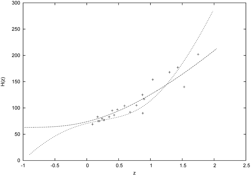
Figure 1. Comparison of experimental data from [38,40,41] for $H(z)$ measured in units of km s${}^{-1}$ Mpc${}^{-1}$ with our predictions for $z_t=0.71$, $q_0=-0.57$ and $H_0=70.5$ (dotted line) and a ΛCDM fit for $H_0=73.8$ and ${\Omega }_{m,0}=0.27$ taken from [31] (dashed line).

6.5.3. Remarks on BAOs and the CMB-shift Parameter

Baryon acoustic oscillations in the early Universe are imprinted as peaks in the late time matter power spectrum (cp. [42]). But the physical interpretation, mainly of the first peak position, depends heavily on the present baryonic and dark matter contents ${\Omega }_{b0}$ resp. ${\Omega }_{m0}$ of the Universe (see Figure 4 in [42]. This issue is usually ignored in the data analyses performed in the literature [43]. But our model, as a unified model for the dark sector of the Universe, is unable to predict ${\Omega }_{m0}$ (for more details cp. Section 6.6) and therefore we cannot at present analyse these peaks. The same argument holds for the CMB-shift parameter (cp. [44]). This issue has been discussed already in our recent paper [15].

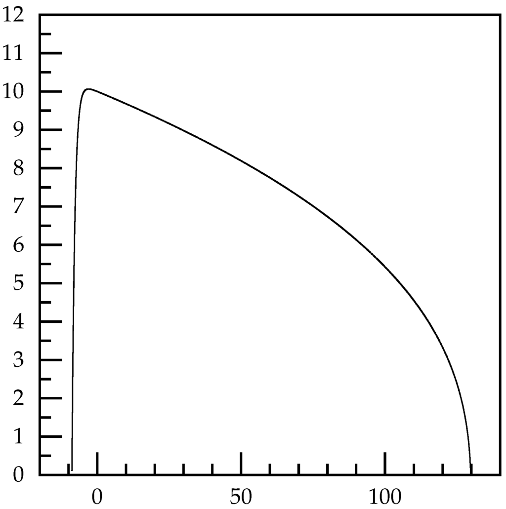
Figure 2. Numerical solution of Equation (232) for $a=10$ and $b=-0.03$.

6.6. Comparison with Alternative Models for Dark Energy

In the following we will sketch how to perform a comparison of our model with alternative models of the dark energy. Any details will be left for the future.

The Friedmann equations, derived from GR including a cosmological “constant” Λ, are for a flat Universe (see e.g., [27])

$$H^2=\frac{8\pi G\rho }{3}+\frac{\Lambda }{3}$$

(197)

$$\frac{\ddot{a}}{a}=-\frac{4\pi G}{3}(\rho +3p)+\frac{\Lambda }{3}$$

(198)

where ρ is the total energy density of the Universe (sum of the matter (M) and dynamical dark energy ($DE$) if we neglect radiation) and, if we assume that matter is described by pressure less dust, p is the (supposed negative) pressure of $DE$

$$\rho ={\rho }_M+{\rho }_{DE},p=p_{DE}<0$$

(199)

Let us now assume that the first Friedmann Equation (197) holds. Then the second Equation (198) can be replaced, as is well known, by the continuity equation

$$\frac{d}{dt}\left(\frac{\Lambda }{8\pi G}+\rho \right)+3H(\rho +p)=0$$

(200)

Note that if we allow a weak time-dependence of Newton’s gravitational constant G the last Equation (200) would have to be generalised (see [45,46]). However, this case will not be discussed here, instead we refer the reader to [46] and the literature cited therein.

At this stage it is important to contrast here two possibilities for the description of the “dark energy” [45]:

• Some kind of fluid described by an equation of state (EoS) $W(z)$

  $$W(z)=\frac{p}{{\rho }_{DE}}$$

  (201)
• A (possibly) time-dependent Λ with a fixed EoS

  $${\rho }_{\Lambda }\equiv \frac{\Lambda }{8\pi G}=-p_{\Lambda }$$

  (202)

Now our Friedmann-like equations are (see Equations (175) and (178))

$$\frac{\ddot{a}}{a}=K_2^{\frac{1}{2}}\tilde{g}(z){(1+z)}^3$$

(203)

and

$$H^2={\left(\frac{K_2}{K_1}\right)}^2{\left(1+\frac{{\tilde{g}}^2(z)}{2}\right)}^2{(1+z)}^2$$

(204)

Comparing the corresponding right hand sides with Equations (197),(198) we obtain two equations for the effective functions ρ, ${\rho }_{\Lambda }$ and p

$$\rho +{\rho }_{\Lambda }=\frac{3H^2}{8\pi G}=\frac{3}{8\pi G}{\left(\frac{K_2}{K_1}\right)}^2{\left(1+\frac{{\tilde{g}}^2(z)}{2}\right)}^2{(1+z)}^2$$

(205)

$$p-{\rho }_{\Lambda }=-\frac{1}{8\pi G}{\left(\frac{K_2}{K_1}\right)}^2{\left(1+\frac{{\tilde{g}}^2(z)}{2}\right)}^2{(1+z)}^2-\frac{1}{4\pi G}{K}_2^{\frac{1}{2}}\tilde{g}(z){(1+z)}^3$$

(206)

In the first scenario we have to put ${\rho }_{\Lambda }=0$ and arrive at two equations for the three functions ${\rho }_M$, ${\rho }_{DE}$ and p. If we suppose that we have no interaction between $CDM$ and $DE$ we have, in addition, local conservation of ${\rho }_M$

$${\dot{\rho }}_M+3H{\rho }_M=0$$

(207)

with the solution

$${\rho }_M={\rho }_{M,0}{(1+z)}^3$$

(208)

From Equations (205), (206) and (208) we easily get an equation for the effective EoS which, however, contains as a free parameter the present value of the energy density of matter ($CDM$ + baryonic matter), ${\rho }_{M,0}$, which is not determined in our unified model for the dark sector of the Universe, i.e., ${\rho }_{M,0}$ is a free parameter in our model (for a very detailed discussion of this issue see [47]). Therefore our model, as any other unified dark fluid model, is not able to predict an EoS for $DE$. However, on the other hand, we can define an EoS $W_D$ for the darkon fluid as a whole

$$W_D=\frac{p}{\rho }=-\frac{1}{3}-\frac{2K_2^{\frac{1}{2}}\tilde{g}(z)(1+z)}{3{\left(\frac{K_2}{K_1}\right)}^2{\left(1+\frac{{\tilde{g}}^2(z)}{2}\right)}^2}$$

(209)

Whether $W_D$ for some z-region shows a phantom-like behaviour ($w_D<-1$) will be left for future considerations.

In the second scenario we have to put ${\rho }_{DE}=p=0$ which corresponds to model II in [46]. We decompose ${\rho }_M$ into its $DM$ and B parts

$${\rho }_M={\rho }_{DM}+{\rho }_B$$

(210)

and take into account the local conservation of ${\rho }_B$ which leads, in the cosmological limit, to (cp. Equation (208))

$${\rho }_B={\rho }_{B,0}{(1+z)}^3$$

(211)

Note that ${\rho }_{B,0}$, in contradistinction to ${\rho }_{M,0}$, is directly observable. Then Equations (205), (206) lead to predictions for ${\rho }_{DM}$ and ${\rho }_{\Lambda }$ for a given set of constants $K_i$ ($i=1,2,3$). More details and their comparison with the results communicated in [46] will be left for the future.

7. Modeling Dark Matter Halos by a Steady State Darkon Fluid

We start with the darkon fluid EOMs in the Eulerian formulation as given in Section 3. By taking their time-independent form (steady state equations) we will derive a nonlinear ordinary differential equation (ODE) for the gravitational potential in the spherically symmetric case. The solutions of this ODE may serve as a model for the dark matter (DM) halos of galaxies. In particular we consider DM-dominated galaxies in which case the halo dominates the galactic gravitational potential and therefore determines the rotational velocity of stars (rotation curves (RCs)).

In subsection 7.1 we derive the nonlinear ODE for the gravitational potential in the spherically symmetric case and the behaviour of their solutions for large distances from the centre of the halo. Then, in subsection 7.2, we present the results of the numerical solutions of this ODE and compare them with the main characteristics of the observational data for the RCs of DM-dominated galaxies.

7.1. Equation for the Gravitational Potential

From the darkon fluid EOMs Equation (73) we obtain immediately the following steady state equations:

Steady state equation for the gravitational field

$$u_k{\partial }_k\left(\frac{g_i}{n}\right)=\frac{g_k}{n}{\partial }_i{u}_k-{\theta }_i$$

(212)

where the auxiliary field ${\theta }_i$ is given by the solution of

$$u_k{\partial }_k{\theta }_i+{\theta }_k{\partial }_i{u}_k=0$$

(213)

Euler equation:

$$u_k{\partial }_k{u}_i=g_i$$

(214)

Continuity equation:

$${\partial }_k(u_{k}n)=0$$

(215)

Next we consider the halos as spherically symmetric objects. Then the vector fields appearing in Equations (212)–(215) take the following form:

$$u_k(\overrightarrow{x})=\frac{x_k}{r}u(r),g_k(\overrightarrow{x})=-\frac{x_k}{r}{\varphi }^{{}^{\prime }}(r)$$

(216)

$${\theta }_k(\overrightarrow{x})=\frac{x_k}{r}\theta (r)$$

where ϕ is the gravitational potential. By using Equation (216) in the steady state equations we obtain from Equation (212)

$$u^2{\left(\frac{{\varphi }^{{}^{\prime }}}{un}\right)}^{{}^{\prime }}=\theta$$

(217)

where θ, obtained by the integration of Equation (213), is given by

$$\theta (r)=-\frac{1}{2}\frac{\gamma }{\alpha u(r)}$$

(218)

For convenience we have chosen to write the integration constant as $-\frac{\gamma }{2\alpha }$. Euler’s Equation (214) leads to the Bernoulli eq.

$$\frac{1}{2}{u}^2=-\varphi$$

(219)

and the solution of the continuity equation gives

$$un=\frac{\alpha }{r^2}$$

(220)

where α is an integration constant.

As in the Lagrangian formulation the vector field $\overrightarrow{\theta }$ is a conserved quantity, we may wonder whether it is possible to connect the integration constants α and γ appearing here and $K_1$ appearing in the cosmological context (see Equation (123)).

We find, in our case,

$${\theta }_k(\overrightarrow{\xi })=-\frac{1}{2}{\xi }_k|\overrightarrow{\xi }|\frac{n_0\gamma }{{\alpha }^2}$$

(221)

This expression has a different $\overrightarrow{\xi }$ dependence from that of the r.h.s. of Equation (123). So, unfortunately, there is no relation between α and γ on one hand and $K_1$ on the other.

We note that the solution (220) produces a singularity at the origin on the r.h.s. of the continuity Equation (215). This singularity might be interpreted as the central black hole of the galaxy (see [47] for the existence of a central black hole in LSB-galaxies). But a black hole describes a sink for any kind of matter. So we get $\alpha <0$ and therefore

$$u<0$$

(222)

Inserting all these expressions into Equation (217) we obtain a ODE

$$\frac{1}{r^2}{(r^2{\varphi }^{{}^{\prime }})}^{{}^{\prime }}=\frac{\gamma }{2r^2}{(-2\varphi )}^{-\frac{3}{2}}$$

(223)

which may be understood as the Poisson equation for a self-consistently determined effective DM mass density ρ

$$4\pi G\rho (r)=\frac{\gamma }{2r^2}{(-2\varphi )}^{-\frac{3}{2}}$$

(224)

Next we switch over to a dimensionless potential ϕ by the substitution

$$\varphi \to {\gamma }^{\frac{2}{5}}\varphi$$

(225)

From the foregoing equations we easily conclude that γ has the dimension $m^5{s}^{-5}$ as it should be.

So, altogether, we end up with a nonlinear, non-autonomous ODE for ϕ

$${(r^2{\varphi }^{{}^{\prime }})}^{{}^{\prime }}=\frac{1}{2}{(-2\varphi )}^{-\frac{3}{2}}$$

(226)

in which ϕ is nonpositive and satisfies the natural boundary conditions

$$\varphi (\infty )=0\text{and}\varphi (1)=-\frac{\eta }{2},\eta >0$$

(227)

We note that the ODE Equation (226) and the first boundary condition ($\varphi (\infty )=0$) are invariant w.r.t. to the scale transformation

$$\varphi (r)\to \tilde{\varphi }(r)\equiv \varphi (\lambda r),\lambda >0$$

(228)

Thus the second boundary condition is necessary to make the solution unique.

To simplify Equation (226) we introduce, instead of ϕ, the function $\psi =-2r\varphi$ which then has to satisfy the ODE

$${\psi }^{{}^{\prime \prime }}=-r^{\frac{1}{2}}{\psi }^{-\frac{3}{2}}(r)$$

(229)

whose positive solutions have to be determined.

Remark: Equation (229) resembles the Thomas–Fermi equation which arises in the self-consistent determination of the potential within a neutral atom. But there are two important differences between these two problems. Besides the negative sign in Equation (229), the function on its r.h.s. is reciprocal to the one appearing in the Thomas–Fermi equation.

To determine the required solutions of Equation (229) let us consider first Equation (229) with the boundary conditions

$$\psi (1)=\eta ,\eta >0\text{and}{\psi }^{{}^{\prime }}=\beta$$

(230)

In this case we can use the following lemma, which is a particular case of a more general theorem derived by S. Taliaferro (see theorem 2.1 in [48])

Lemma [48]. Let $\psi (r)$ be a positive solution of Equation (229) satisfying Equation (230) for fixed $\eta >0$ and an arbitrary real number β. Then there exists $r_2$, satisfying $1<r_2<\infty$ such that ${lim}_{r\to r_2}\psi (r)=0$ and $\psi (r)$ cannot be continued past $r_2$ as a twice continuously differentiable solution of Equation (229).

To use this lemma to the study of properties of required solutions of Equation (226) it is advantageous to perform first the transformation

$$r\to x\equiv logr,\psi (r)\to \phi (x)\equiv e^{-x}\psi (e^x)$$

(231)

Then Equation (229) with the boundary conditions Equation (230) gets transformed into the following autonomous ODE

$${\phi }^{{}^{\prime \prime }}(x)+{\phi }^{{}^{\prime }}(x)=-{\phi }^{-\frac{3}{2}}(x)$$

(232)

with the boundary conditions

$$\phi (0)=a,a>0\text{and}{\phi }^{{}^{\prime }}(0)=b,b\in R^1$$

(233)

where a and b are dimensionless numbers.

By Equation (231) the lemma may be translated to the following statement about φ: For fixed a and arbitrary b we have ${lim}_{x\to x_2}\phi (x)=0$, where $x_2\equiv log{r}_2$, and φ cannot be continued past $x_2$. Equations (232) and (233) are together equivalent to the integral equation

$$\phi (x)=a+b\left(1-e^{-x}\right)-{\int }_0^{x}ds\left(1-e^{s-x}\right){\phi }^{-\frac{3}{2}}(s)$$

(234)

Using the relation

$$\varphi (r)=-\frac{1}{2}\phi (logr)$$

(235)

Equation (234) may be rewritten as an integral equation for $\varphi (r)$:

$$\begin{gathered} \varphi (r)=-\frac{1}{2r}{\int }_0^{r}ds{(-2\varphi (s))}^{-\frac{3}{2}}-\frac{1}{2}{\int }_r^{\infty }\frac{ds}{s}{(-2\varphi (s))}^{-\frac{3}{2}} \\ +\frac{1}{2}\left(-a-b+{\int }_1^{\infty }\frac{ds}{s}{(-2\varphi (s))}^{-\frac{3}{2}}\right) \\ +\frac{1}{2r}\left(b+{\int }_0^{1}ds{(-2\varphi (s))}^{-\frac{3}{2}}\right) \end{gathered}$$

which is cast in such a form that the first line contains the usual integral of the Poisson equation, the second line a constant and the third one a term being proportional to $\frac{1}{r}$.

But the latter is in conflict with the original ODE Equation (226). The reason is that the transformation Equation (235) becomes singular at $r=0$. Therefore the coefficient of $\frac{1}{r}$ has to vanish which fixes the value of b at

$$b=b_c\equiv -{\int }_0^{1}ds{(-2\varphi (s))}^{-\frac{3}{2}}=-{\int }_{-\infty }^{0}ds{e}^s{\phi }^{-\frac{3}{2}}(s)$$

(237)

But the lemma given above holds for any b, and so in particular also for $b=b_c$. Thus, due to the relation Equation (235), it holds also for $\varphi (r)$ ie. ${lim}_{r\to r_2}\varphi (r)=0$ and so $\varphi (r)$ cannot be continued past $r_2$.

Next we return to looking at solutions φ of Equation (232). We know from the results given above that

• we have to find a positive solution φ at least for $0<x<x_2$ with $\phi (x_2)=0$.
• we have to vary b until it reaches a value $b_c$ which corresponds to

  $$b_c=-{\int }_{-\infty }^{0}ds{e}^s{\phi }^{-\frac{3}{2}}(s)$$

  (238)

  leading to

  $${\phi }^{{}^{\prime }}\le -e^{-x}{\int }_{-\infty }^{x}ds{e}^{s-x}{\phi }^{-\frac{3}{2}}(s)<0\text{for}\text{all}b\le b_c$$

  (239)

To relate the solutions of Equation (232) to the RCs $v(r)$ of a DM-dominated galaxy we recall that $v(r)$ is determined from the equality of the centripetal acceleration and the gravitational force acting on a star in circular motion [49]

$$\frac{v^2(r)}{r}={\gamma }^{\frac{2}{5}}{\varphi }^{{}^{\prime }}(r)$$

(240)

where the factor ${\gamma }^{\frac{2}{5}}$ arises due to the dimensionlessness of ϕ after the substitution Equation (225). Then, using (235) we can determine v in terms of the derivative of φ

$$v^2(r)=-\frac{1}{2}{\gamma }^{\frac{2}{5}}{\phi }^{{}^{\prime }}{(x)|}_{x=logr}$$

(241)

7.2. Predictions versus Observations

To begin with we would like to discuss how to fix, at least in principle, scales for distances and velocities. Due to the dilation symmetry of our model (see Equation (228)) we have no intrinsic scale for distances. A scale for velocities may be chosen by fixing the value of the dimensionfull constant γ. However, γ, being an integration constant, is an extrinsic parameter. So our model does not possess any intrinsic scale for distances or for velocities. To get intrinsic scales we must introduce dilation symmetry breaking terms into the Lagrangian. We can do this either by taking into account the coupling to baryonic matter and/or by adding within the gravitational coupling Equation (26) higher order derivative terms as indicated in Equation (29).

So, for the present form of our model, we get the required scales by fixing two extrinsic parameters. For velocities we have to fix γ. For distances we have to fix the scale parameter λ in Equation (228) or, equivalently, put $x=0$ in Equation (233) which fixes $r=R$ where R is the chosen unit of length. Thus, to fit observational data for the RCs of any given galaxy, we would have to perform a best fit for γ, R and the dimensionless “initial” value a in Equation (233). However, as we view the present model only as a first building block for a new theory (cp. Section 9) we think it is premature to perform any “least square fits” to the data. Thus we have only checked whether there is a general qualitative agreement of the predictions of our model with the data. We have done this by fitting the extrinsic parameters γ and R to one particular galaxy at a fixed value of a. Note that the choice of a fixes $b_c$.

More detailed discussion has been postponed until we have generalised our model to a general covariant one as suggested in Section 9.

We have solved numerically the nonlinear differential Equation (232) for $\phi (x)$ by choosing the initial conditions Equation (233) with $a=10$ and $b\le -0.03$. The main result is the abrupt change of the character of the graphs for $\phi (x)$ at negative x-values at the critical b-value $b_c$ given approximately by

$$b_c=-0.031475314466$$

(242)

For $b>b_c$ the graph of $\phi (x)$ crosses the x-axis at some $x_0<0$ where $x_0$ is an increasing function of b. We believe, although this is numerically hard to verify, that $x_0\to -\infty$ for b decreasing to $b_c$. For $x<x_0$ the solution becomes complex valued. This behaviour is illustrated in Figure 2 ($b=-0.03$) and Figure 3 ($b=b_c$).

On the other hand for $b<b_c$ the graph of $\phi (x)$ starts to rise rapidly at some $x<0$ and goes to infinity. This behaviour is clear from Figure 4 ($b=-0.032$).

Furthermore, from the plot of ${\phi }^{{}^{\prime }}(x)$ for $b=-0.032$ (Figure 5) we see that ${\phi }^{{}^{\prime }}(x)<0$ for all $x\in R^1$.

The behaviour of the graphs of φ and ${\phi }^{{}^{\prime }}$ for $b\ge b_c$ resp. $b<b_c$ as shown in Figure 2, Figure 3, Figure 4 and Figure 5 strongly suggests that the $b_c$ obtained numerically in Equation (242) is, modulo numerical fine tuning, indeed identical to the expression for $b_c$ derived in Section 7.1 as the correct b-value for modeling halos by means of the solution of the boundary value problem Equations (232),(233) for $a=10$.

Hence we have to compare qualitatively the RCs calculated for $b=b_c$ with observational data. For that we plot in Figure 6 and Figure 7 the rotational velocities $v(r)$ determined from Equation (241). In Figure 6 we show the behaviour of $v(r)$ at small radii with the extrinsic parameters ${\gamma }^{\frac{1}{5}}$, resp. R fitted, for fixed $a=10$ to the RC of the dwarf galaxy UGC 8490 (data taken from [50]). Figure 7 shows the global behaviour of $v(r)$ in dimensionless units.

Figure 3. Numerical solution of Equaiton (232) for $a=10$ and $b=b_c$ (thick line) compared with our approximation Equaiton (243) (thin line).

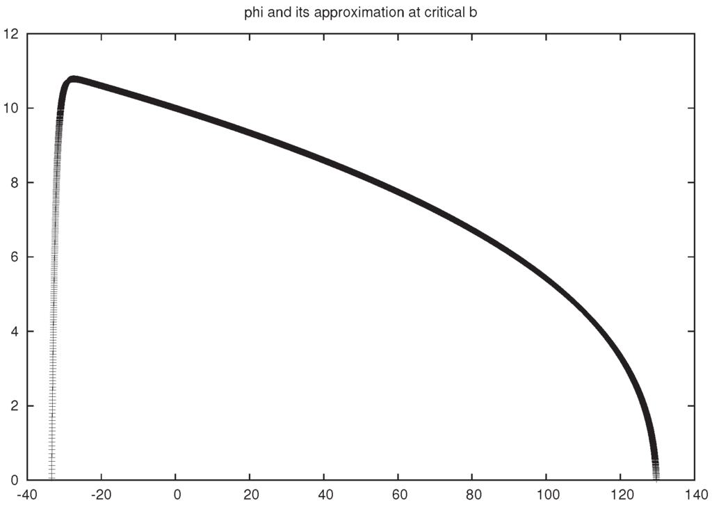
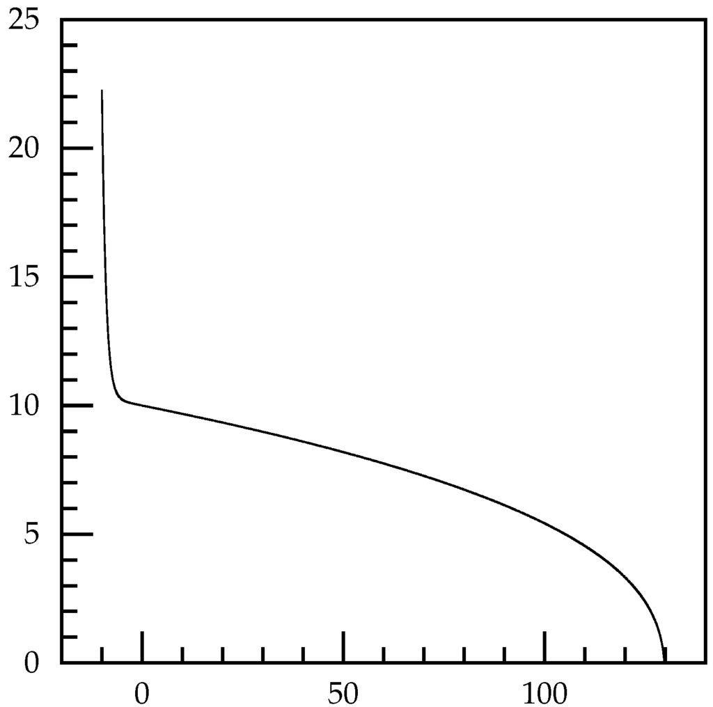
Figure 4. Numerical solution of (232) for $a=10$ and $b=-0.032$.

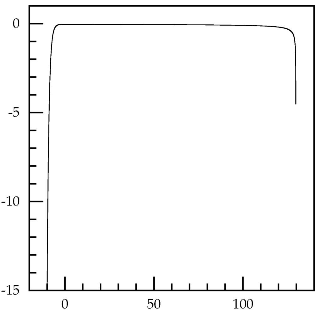
Figure 5. Numerically obtained ${\phi }^{{}^{\prime }}$ for $a=10$ and $b=-0.032$.

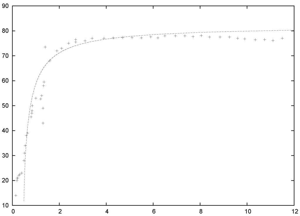
Figure 6. Numerically determined plot of the darkon fluid contribution to the rotational velocity $v(r)$ (in $km{s}^{-1}$) at small radii (in $kpc$) for $b=b_c$, ${\gamma }^{\frac{1}{5}}=615km{s}^{-1}$ and $R=4\times {10}^{11}kpc$. Compared with the RC of UGC 8490 (data from [50]).

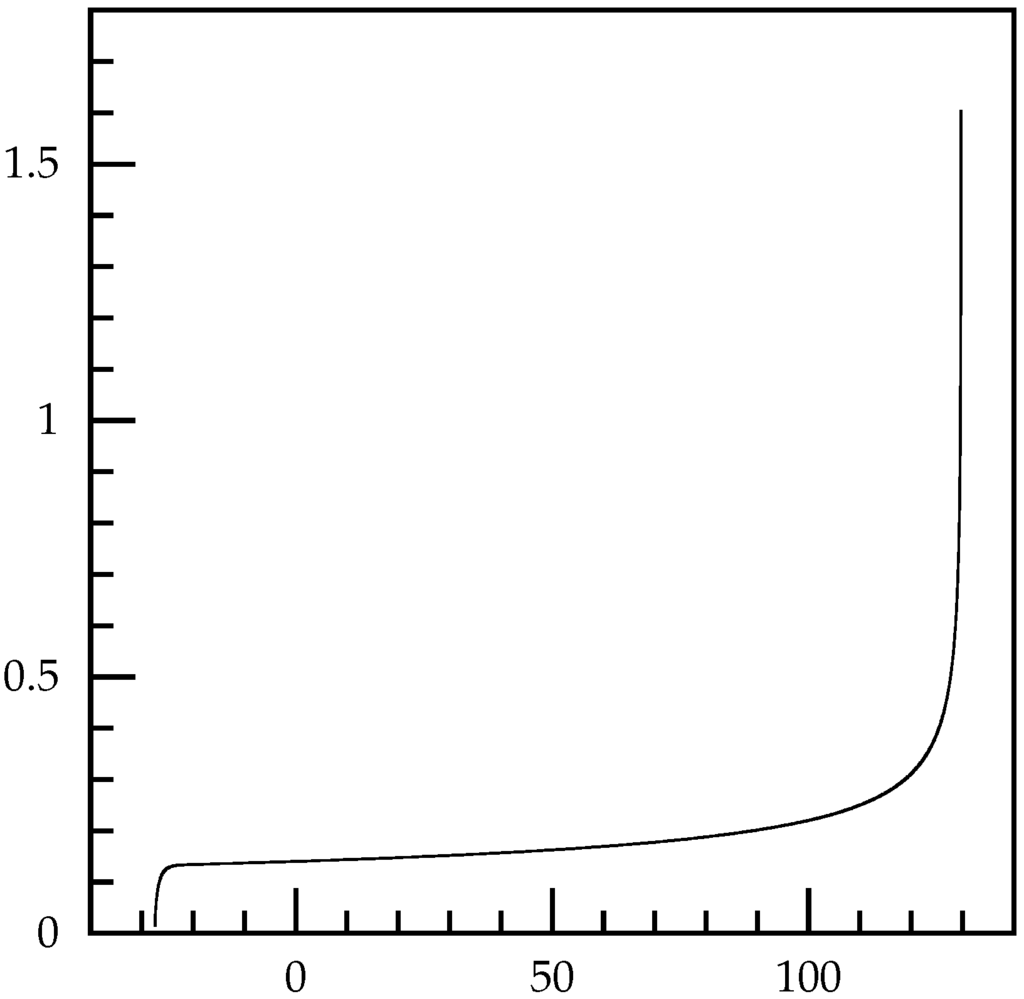
Figure 7. Global behaviour of the rotational velocity $v(r)$ for $b=b_c$ plotted as a function of $x=logr$.

The graphs for the darkon fluid contribution to the RCs given in Figure 6 and Figure 7 show the following qualitative characteristics when compared with observational data on DM haloes (for a very recent review see [51])

• They start at a radius $r_1\sim 0$ and rapidly increase reaching $v(r)\sim 76km{s}^{-1}$ at $r\sim 4kpc.$ (Figure 6).
• Beyond this increase our model predicts a rather flat, but still very slowly increasing behaviour for the RCs until extremely large radii. This is basically in agreement with all observations according to which the RCs of a galaxy stay approximately constant after attaining a maximum at about 5 kpc [52]. This statement is true, in particular, for the DM-dominated galaxies: the LSB-galaxies (cp. the RCs reproduced in [53] and in Figure 3 and Figure 4 of [54]) and dwarf galaxies (cp. [55] and the RCs reproduced in [50]).
  The behaviour of $\phi (x)$ within this flat-like region can be well approximated by (see Figure 3)

  $$\phi (x)\sim f(x)={(2.5)}^{0.4}{(c-x)}^{0.4}$$

  (243)

  where $c\sim 126.5$ has been fixed by $f(0)=10$. Then we obtain $f^{\prime }(0)\sim -0.03162$, which is a good approximation for $b_c$ Equation (242). $f(x)$ is the solution of the ODE

  $$f^{\prime }(x)=-f^{-\frac{3}{2}}(x)$$

  (244)

  and so is an approximate solution of the ODE Equation (232) if ${\phi }^{\prime }\sim$ const.
• They terminate at an extremely large radius roughly given by $r_2\sim e^{130}$ with a diverging RC as $r\to r_2$.
  Of course, this contradicts all observations. But the size of $r_2$ is clearly orders of magnitude larger than the size of the visible part of the Universe: In the FRW model the size $R_0$ of the Universe is given by $R_0=0.5c{t}_0$ [56], where $t_0\sim 13.7$ Gyr is the age of the Universe [49]. Thus we obtain $R_0\sim 2.1$ Gpc. The choice $R=4.{10}^{14}pc$ in Figure 6 gives $r_2\sim {10}^{71}$ pc, which is about 62 orders of magnitude larger than $R_0$.

We conclude that this highly unphysical behaviour of $v(r)$ as $r\to r_2$ is possibly a consequence of considering only an isolated halo. We expect an improvement of this situation if we embed the halo in the time-dependent darkon fluid (to be done by an appropriate generalization of the considerations in Section 8).

8. Influence of the Cosmic Expansion on Binary Systems

In the following we consider two astrophysical objects, one of large mass M (e.g., the sun) and another one of small mass $m\ll M$ (e.g., a planet) embedded in the time dependent darkon fluid which, asymptotically behaves like the cosmological solution (see section 6.2). We would like to assess the change of Newton’s force of attraction between the two bodies due to the presence of the darkon fluid. To be specific we approximate this binary system by a point-like test particle of mass m which moves in the time-dependent gravitational potential created by a point-like mass M and the overall darkon fluid considered in the rest system of the heavy mass M.

Within GR the corresponding problem is to find, as a solution of Einstein’s equation, an interpolation between the Schwarzschild and the FLRW metric. Then the motion of the test particle is the geodesic motion in this metric. A solution to this problem has been given in a very recent paper [57] (see also the recent review [58] and the literature quoted therein, which covers also the history of this problem starting with the paper by Mc Vittie in 1933 [59]). In the Newtonian limit one obtains for the EOM of the test particle (see [57])

$${\ddot{x}}_i=\frac{\ddot{a}}{a}{x}_i-\frac{GM}{r^3}{x}_i$$

(245)

It turns out that the correction to Newton’s law by the present accelerated expansion is completely negligible within the solar system (see section III A in [58]).

In the following we will sketch the ideas how to obtain the correction to Newton’s law for our model.

We start with the EOMs given in 3.4 with a gravitational potential

$$\varphi (r,t)={\varphi }_D(r,t)-\frac{GM}{r}$$

(246)

where ${\varphi }_D$ represents the darkon fluid contribution. Then we obtain, in the spherically symmetric case, the EOMs

$$\dot{w}+{(uw)}^{{}^{\prime }}=0$$

(247)

$$\dot{u}+\frac{1}{2}{(u^2)}^{{}^{\prime }}=-{\varphi }^{{}^{\prime }}$$

(248)

$${(r^2{\varphi }_D^{{}^{\prime }})}^{·}+u{(r^2{\varphi }_D^{{}^{\prime }})}^{{}^{\prime }}=w\theta$$

(249)

$$\dot{\theta }+{(u\theta )}^{{}^{\prime }}=0$$

(250)

where the functions u and θ are given by Equation (216) generalized to the time-dependent case and we have defined $w=r^{2}n$. A dot represents ${\partial }_t$ and a slash ${\partial }_r$. Next we have to solve Equations (247)–(250) with the following boundary conditions:

• for $r\to \infty$ the functions $w,u,{\varphi }_D$ and θ attain their cosmological limits defined in 6.1

  $$w(r,t)=\frac{r^2{n}_0}{a^3(t)},u(r,t)=r\frac{\dot{a}(t)}{a(t)}$$

  (251)

  $${\varphi }_D(r,t)=-\frac{r^2}{2}\frac{g(a(t))}{a^3(t)},\theta (r,t)=-\frac{K_1}{n_0{a}^2(t)}r$$

  They are solutions of Equations (247)–(250) if a and g satisfy the cosmological Equations (121), (122).
• for $r\to 0$ we require that

  $$r{\varphi }_D\to 0$$

  (252)

  leading, if inserted into the EOMs Equations (247)–(250), to the following behavior of u, w, θ and ${\varphi }_D$ for $r\to 0$

  $$u(r,t)\sim \beta r^{-\frac{1}{2}}\text{with}\beta =\pm {(2GM)}^{\frac{1}{2}}$$

  (253)

  $$w(r,t)\sim r^{\frac{1}{2}}{f}_w\left(t-\frac{2}{3\beta }{r}^{\frac{3}{2}}\right)$$

  (254)

  $$\theta (r,t)\sim r^{\frac{1}{2}}{f}_{\theta }\left(t-\frac{2}{3\beta }{r}^{\frac{3}{2}}\right)$$

  (255)

  $$\varphi {{}^{\prime }}_D\sim \frac{2}{5\beta }{r}^{\frac{1}{2}}(f_w{f}_{\theta })\left(t-\frac{2}{3\beta }{r}^{\frac{3}{2}}\right)$$

  (256)

  where the functions $f_w$, $f_{\theta }$ and the sign of β still have to be determined.

If it turns out that it is not be possible to obtain analytic expressions for these functions, one should try to find an approximation involving a two-scale perturbation expansion. The small spatial scale will be given by the size of the binary system and the large one by the cosmic scale. This problem is currently under consideration.

9. Outlook for a General Covariant Theory

The Poincare algebra treats spatial and time variables on the same footing. Then its enlargement by dilations has necessarily a dynamical exponent $z=1$ (cp. [60]). But in our model we have anisotropic scaling with $z=\frac{5}{3}$. Therefore, an enlargement of the Milne gauge group Equation (24) to arbitrary space-time diffeomorphisms (Diff) as the symmetry group for a generalized darkon fluid model seems to be forbidden. But the dilation symmetry with $z=\frac{5}{3}$ was an emergent symmetry and not an input of our model. So we should look for a general covariant generalization of our model without imposing any form of scale symmetry.

To do this we have to first restore the Milne gauge invariance for the Eulerian action Equation (56) by undoing the gauge fixing Equation (41) leading to

$$S=\frac{1}{4\pi G}\int dt{d}^{3}x\left(4\pi Gn{q}_i(D_t{u}^i-g^i)-\theta ({\partial }_{t}n+{\partial }_k(n{u}^k))+n\alpha D_t\beta \right)+S_{field}$$

(257)

with the spatial metric given by ${\eta }_{ij}={\delta }_{ij}$ and $S_{field}$ is determined by the expression (31).

Now we propose the following action as the Diff-generalization of Equation (257)

$$D_{diff}=\frac{1}{4\pi G}\int d^{4}x\sqrt{-g}\left(4\pi Gn{\tilde{q}}_{\nu }{u}^{\lambda }{\Delta }_{\lambda }{u}^{\nu }-\theta {\Delta }_{\lambda }(n{u}^{\lambda })+n\alpha u^{\lambda }{\partial }_{\lambda }\beta \right)+S_{EH}$$

(258)

where we have used the following notation (in units with $c=1$): g is the determinant of the covariant space-time metric $g_{\mu \nu }$ with the invariant line element

$$d{s}^2=g_{\mu \nu }d{x}^{\mu }d{x}^{\nu }$$

(259)

and ${\Delta }_{\lambda }$ denotes the covariant derivative

$${\Delta }_{\lambda }{u}^{\nu }\equiv {\partial }_{\lambda }{u}^{\nu }+{\Gamma }_{\lambda \sigma }^{\nu }{u}^{\sigma }$$

(260)

Here ${\Gamma }_{\lambda \sigma }^{\nu }$ is the corresponding Levi–Civita connection, n is the scalar particle density and $u^{\lambda }$ the four-velocity. θ, α and β are scalar fields. The vector field ${\tilde{q}}_{\mu }$ will be deduced, as given below, from the Milne scalar $q_i$. Finally the last term in Equation (258), which is the Diff-generalisation of the last term in Equation (257), is the Einstein–Hilbert action given by

$$S_{EH}=-\frac{1}{16\pi G}\int d^{4}x\sqrt{-g}R$$

(261)

where R is the Ricci-scalar.

To understand Equation (258) as a Diff-generalization of Equation (257) we consider the limiting case

$$u^0\to 1,g_{\mu \nu }\to {\eta }_{\mu \nu }({\eta }_{\mu \nu }\equiv \text{diag}(-1,1,1,1,))$$

(262)

$${\Gamma }_{\lambda \sigma }^{\nu }\to 0\text{except}{\Gamma }_{00}^i\to -g^i$$

which are the leading terms known from the Newtonian weak field limit of General Relativity (GR) $g_{\mu \nu }={\eta }_{\mu \nu }+h_{\mu \nu },|h_{\mu \nu }|\ll 1$ and an expansion of $h_{\mu \nu }$ in inverse powers of c. Here $g^i$ is the nonrelativistic gravitational field as used in Equation (257).

To construct the vector field ${\tilde{q}}_{\mu }$ we proceed in two steps:

• By means of a Lorentz transformation we promote the Milne scalar $q_i$ ($i=1,2,3)$ to $q_{\underline{\alpha }}$ ($\underline{\alpha }$ = 0,1,2,3), which is a scalar field w.r.t. Diff but a contravariant space-like vector field, labeled by $\underline{\alpha }$, in tangent space.
• By means of tetrads $E_{\mu }^{\underline{\alpha }}$ (known from teleparallel gravity, cp. [61]) we transform $q_{\underline{\alpha }}$ to the four-vector field ${\tilde{q}}_{\mu }$

  $$q_{\underline{\alpha }}\to {\tilde{q}}_{\mu }\equiv q_{\underline{\alpha }}{E}_{\mu }^{\underline{\alpha }}$$

  (263)

The tetrads $E_{\mu }^{\underline{\alpha }}$ transform like a contravariant vector w.r.t. Diff by changing the Greek index and like a four-vector w.r.t. Lorentz transformations by changing the underlined Greek index. The tetrads are related to the metric tensor by

$$g_{\mu \nu }={\eta }_{\underline{\alpha }\underline{\beta }}{E}_{\mu }^{\underline{\alpha }}{E}_{\nu }^{\underline{\beta }}$$

(264)

So the limit $g_{\mu \nu }\to {\eta }_{\mu \nu }$ corresponds to $E_{\mu }^{\underline{\alpha }}\to {\delta }_{\mu }^{\underline{\alpha }}$ and so to ${\tilde{q}}_{\mu }\to q_{\underline{\mu }}$ . Therefore we obtain, in the limiting case, for the individual terms in Equation (258)

$${\tilde{q}}_{\nu }{u}^{\lambda }{\Delta }_{\lambda }{u}^{\nu }\to q_i(D_t{u}^i-g^i)$$

$${\Delta }_{\lambda }(n{u}^{\lambda })\to {\partial }_{t}n+{\partial }_k(n{u}^k),u^{\lambda }{\partial }_{\lambda }\beta \to D_t\beta$$

(265)

in agreement with Equation (257).

What about possible scaling properties of the action Equation (258)? The generators of Diff do not form a closed algebra together with the generators of anisotropic scaling transformations

$$t\to t^{*}={\lambda }^{z}t,x_i\to x^{*i}=\lambda x^i$$

(266)

A closed algebra can be obtained only if the rigid transformations (266) are replaced by local ones (Weyl transformations). But the Einstein–Hilbert action (261) does not respect the Weyl symmetry (for that we would have to replace Equation (261) by the Weyl action (cp. [62] and the literature cited therein)). So we can only expect, like in Horava gravity [63], to find scale invariant solutions in the ultraviolet or in the infrared regime. Any further consequences of this new ansatz Equation (258) for a general covariant darkon fluid still have to be worked out. In particular we are interested in the cosmological implications. But due to the larger number of gauge fields in the action (instead of the three gravitational fields $g^i$ we have now ten fields of the metric tensor $g_{\mu \nu }$) we will obtain cosmological EOMs other than the ones studied so far. In particular we will obtain a prediction for the Hubble parameter $h(z)$ which would probably be different from Equation (180). Therefore nothing can be said at the moment about the asymptotic behaviour of $h(z)$.

10. Conclusions and Outlook

In the present paper we have reviewed our recent results on the darkon-fluid model which is, as outlined in Section 9, a first building block for a new general covariant theory describing the dark sector of the Universe. The model involves new physics by using nonrelativistic massless particles with a nonstandard coupling to the gravitational field. The model, which contains no free parameters in its Lagrangian, predicts qualitatively correct values of the late time cosmic acceleration as well as the flat behaviour of galactic rotation curves. These successes encourage us to continue our work. We have to work out the astrophysical implications of the covariant theory and have to compare them with the predictions of the present model and with observational data.

So the main open topics of research are:

• Derive the EOMs of the covariant theory.
• Restrict the EOMs to the cosmological regime and compare their predictions with the present model. Perform a best fit to the Hubble parameter resp. distance moduli data.
• Enlarge the covariant model by adding baryonic matter.
• Look for the solutions of the spherically symmetric but time dependent EOMs which attain for large distances their cosmological limits.
• Apply the results to

  –

  modeling of halos,

  –

  solar system tests.

• Quantization of the Hamiltonian dynamics for the darkon fluid as a whole or for the cosmological dynamics.
• Answer the question whether the present model is the nonrelativistic limit of the covariant theory in a strict sense.
• Discuss higher order derivative terms within the covariant theory.

These problems are currently under investigation. We hope to be able to present our results soon.

References

- Buchert, Th.; Räsänen, R. Backreaction in late-time cosmology. 2012; arXiv: 1112.5335v1, [astro-ph.CO]. [Google Scholar]
- Roos, M. Astrophysical and cosmological probes of dark matter. 2012; arXiv: 1208.3662v2, [astro-ph.CO]. [Google Scholar]
- Tsujikawa, S. Dark energy: Investigation and modeling. 2010; arXiv: 1004.1493v1, [astro-ph.CO]. [Google Scholar]
- Li, M.; Li, X.-D.; Wang, S.; Wang, Y. Dark energy. Com. Theor. Phys. 2011, 56, 525–604. [Google Scholar] [CrossRef]
- Bamba, K.; Capozziello, S.; Nojiri, S.; Odintsov, S. Dark energy cosmology: The equivalent description via different theoretical models and cosmography tests. 2012; arXiv: 1205.3421.v3, [gr-qc]. [Google Scholar]
- Martin, J. Everything you always wanted to know about the cosmological constant problem (but were afraid to ask). 2012; arXiv: 1205.3365v1, [astro-ph.CO]. [Google Scholar]
- Garrett, K.; Duda, G. Dark matter: A primer. Adv. Astron. 2011. Article ID 968283. [Google Scholar] [CrossRef]
- De Block, W. The core-cusp problem. Adv. Astron. 2010. Article ID 789293. [Google Scholar] [CrossRef]
- Kroupa, P. The dark matter crisis: falsification of the current standard model of cosmology. 2012; arXiv: 1204.2546v2, [astro-ph.CO]. [Google Scholar]
- Milgrom, M. A modification of the Newtonian dynamics as an alternative to the hidden mass hypothesis. Astrophys. J. 1983, 270, 365–370. [Google Scholar] [CrossRef]
- Famaey, B.; McGaugh, S. Modified newtonian dynamics: A review. 2011; arXiv: 1112.3960v2, [astro-ph.CO]. [Google Scholar]
- Moffat, J. Scalar-tensor-vector gravity theory. J. Cosmol. Astropart. Phys. 2006, 004, 1–18. [Google Scholar] [CrossRef]
- Moffat, J.; Toth, V. Modified Gravity: Cosmology without dark matter or Einstein’s cosmological constant. 2012; arXiv: 0710.0364v7, [astro-ph]. [Google Scholar]
- Brownstein, J.; Moffat, J. Galaxy rotation curves without nonbaryonic dark matter. Astrophys. J. 2006, 636, 721–741. [Google Scholar] [CrossRef]
- Stichel, P.; Zakrzewski, W. Can cosmic acceleration be caused by exotic massless particles? Phys. Rev. D. 2009, 80, 083513. [Google Scholar] [CrossRef]
- Stichel, P.; Zakrzewski, W. Self-gravitating darkon fluid with anisotropic scaling. Eur. Phys. J. C. 2010, 70, 713–721. [Google Scholar] [CrossRef]
- Stichel, P.; Zakrzewski, W. Darkon fluid—a model for the dark sector of the Universe? Int. J. Geom. Meth. Mod. Phys. 2012, 9, 1261014. [Google Scholar] [CrossRef]
- Negro, J.; del Olmo, M.; Rodriguez-Marco, A. Nonrelativistic conformal groups. J. Math. Phys. 1997, 38, 3786–3809. [Google Scholar] [CrossRef]
- Milne, E. Newtonian expanding Universe. Quart. J. Math. (Oxford Ser.) 1934, 5, 64, (reprinted in Gen. Rel. Grav. 2000, 32 1939–1948). [Google Scholar] [CrossRef]
- Bennett, A. Lagrangian Fluid Dynamics; Cambridge University Press: Cambridge, UK, 2006. [Google Scholar]
- Jackiw, R.; Nair, V.; Pi, S.; Polychronakos, A. Perfect fluid theory and its extensions. J. Phys. A. 2004, 37, R327–R432. [Google Scholar] [CrossRef]
- Buchert, T. An exact Lagrangian integral for the Newtonian gravitational field strength. Phys. Lett. A. 2006, 354, 8–14. [Google Scholar] [CrossRef]
- Weyssenhoff, J.; Raabe, A. Relativisitic dynamics of spin-fluids and spin-particles. Acta Phys. Pol. 1947, IX, 7–18. [Google Scholar]
- Klauder, J. Enhanced quantum procedures that resolve difficult problems. 2012; arXiv: 1206.4017, [hep-th]. [Google Scholar]
- Hojman, S. The construction of a Poisson structure out of a symmetry and a conservation law of a dynamical system. J. Phys. A 1996, 29, 667–674. [Google Scholar] [CrossRef]
- Herrera, M.; Hojman, S. Non-standard Construction of Hamiltonian Structure and of the Hamilton-Jacobi equation. 2000; arXiv: math-ph/0008019. [Google Scholar]
- Weinberg, S. Cosmology; Oxford University Press: New York, NY, USA, 2008. [Google Scholar]
- McCrea, W. Cosmology. Rep. Progr. Phys. 1953, 16, 321–363. [Google Scholar] [CrossRef]
- Liddle, A. An Introduction to Modern Cosmology; Wiley: Chichester, GB, USA, 2003. [Google Scholar]
- Faroog, O.; Mania, D.; Ratra, B. Hubble parameter measurement constraints on dark energy. 2012; arXiv: 1211.4253, [astro-ph.CO]. [Google Scholar]
- Moresco, M.; Verde, L.; Pozetti, L.; Jimenez, R.; Cimatti, A. New constraints on cosmological parameters and neutrino properties using the expansion rate of the Universe to z ∼ 1.75. 2012; arXiv: 1201.6658, [astro-ph.CO]. [Google Scholar]
- Guimaraes, A.; Cunha, J.; Lima, J. Bayesian analysis and constraints on kinematic models from union SNIa. J. Cosmol. Astropart. Phys. 2009, 10, 0910. [Google Scholar] [CrossRef]
- Giostri, R.; Vargas dos Santos, M.; Waga, I.; Reis, R.; Calvao, M.; Lago, B. From cosmic deceleration to acceleration: new constraints from SNIa and BAO/CMB. 2012; arXiv: 1203.3213, [astro-ph.CO]. [Google Scholar]
- Seikel, M.; Yahya, S.; Maartens, R.; Clarkson, C. Using H(z) data as a probe of the concordance model. 2012; arXiv: 1205.3431, [astro-ph.CO]. [Google Scholar]
- Shafieloo, A.; Kim, A.; Linder, E. Gaussian process cosmography. 2012; arXiv: 1204.2272, [astro-ph.CO]. [Google Scholar]
- Suzuki, N.; Rubin, D.; Lidman, C.; Aldering, G.; Amanullah, R.; Barbary, K.; Barrientos, L.; Botyanski, J.; Brodwin, M.; Connolly, N.; et al. The hubble space telescope cluster supernova survey: V. improving the dark energy constraints above z > 1 and building an early-type-hosted supernova sample. Astrophys. J. 2012, 746, 85. [Google Scholar] [CrossRef]
- Wei, H. Observational constraints on cosmological models with the updated long gamma-ray bursts. J. Cosmol. Astropart. Phys. 2010, 1008, 020. [Google Scholar] [CrossRef]
- Liang, N.; Wu, P.; Zhang, S. Constraints on cosmological models and reconstructing the acceleration history of the universe with gamma-ray burst distance indicators. Phys. Rev. D. 2010, 81, 083518. [Google Scholar] [CrossRef]
- Gaztanaga, E.; Cabre, A.; Hui, L. Clustering of Luminous Red Galaxies IV: Baryon Acoustic Peak in the Line of Sight Direction and a Direct Measurement of H(z). Mon. Not. R. Astron. Soc. 2009, 399, 1663. [Google Scholar] [CrossRef]
- Stern, D.; Jimenez, R.; Verde, L.; Kamionkowski, M.; Stanford, S. Cosmic chronometers: Constraining the equation of state of dark energy. I: H(z) measurements. J. Cosmol. Astropart. Phys. 2010, 02, 008. [Google Scholar] [CrossRef]
- Moresco, M.; Cimatti, A.; Jimenez, R.; Pozetti, L.; Zamorani, G.; Bolzonella, M.; Dunlop, J.; Lamareille, F.; Mignoli, M.; Pearce, H.; et al. Improved constraints on the expansion rate of the Universe up to z ∼ 1.1 from the spectroscopic evolution of cosmic chronometers. 2012; arXiv:1201.3609, [astro-ph.CO]. [Google Scholar]
- Montanari, F.; Durrer, R. An analytic approach to baryon acoustic oscillations. Phys. Rev. D. 2011, 84, 023522. [Google Scholar] [CrossRef]
- Xia, J.; Vitagliano, V.; Liberati, S.; Viel, M. Cosmography beyond standard candles and rulers. 2012; arXiv: 1103.0378v3, [astr-ph.CO]. [Google Scholar]
- Kunz, M.; Liddle, A.; Parkinson, D.; Gao, C. Constraining the dark fluid. Phys. Rev. D 2009, 80, 083533. [Google Scholar] [CrossRef]
- Sola, J. Cosmologies with a time dependent vacuum. J. Phys. Conf. Ser. 2011, 283, 012033. [Google Scholar] [CrossRef]
- Fritzsch, H.; Sola, J. Matter non-conservation in the universe and dynamical dark energy. 2012; arXiv:1202.5097, [hep-ph]. [Google Scholar]
- AAmendola, L.; Kunz, M.; Motta, M.; Saltas, I.; Sawicki, I. Observables and unobservables in dark energy cosmologies. 2012; arXiv: 1210.0439, [astro-ph.CO]. [Google Scholar]
- Taliaferro, S. On the positive solutions of y+ϕ(t)y-λ = 0. Nonlin. Anal.-Theor. 1978, 2, 437–446. [Google Scholar] [CrossRef]
- Binney, J.; Tremaine, S. Galactic Dynamics; Princeton University Press: Princeton, NJ, USA, 2008. [Google Scholar]
- O’ Brien, J.; Mannheim, P. Fitting dwarf galaxy rotation curves with conformal gravity. 2011; arXiv: 1107.5229, [astro-ph.CO]. [Google Scholar]
- Taylor, J. Dark Matter halos from the inside out. Adv. Astron. 2011. Article ID 604898. [Google Scholar] [CrossRef]
- Roos, M. The evidence from astronomy, astrophysics and cosmology. 2010; arXiv:1001.0316, [astro-ph.CO]. [Google Scholar]
- Magana, J.; Matos, T.; Robles, V.; Suarez, A. A brief review of the scalar field dark matter model. 2012; arXiv: 1201.6107, [astro-ph.CO]. [Google Scholar]
- Mannheim, P.; O’Brien, J. Fitting galactic rotation curves with conformal gravity and a global quadratic potential. Phys. Rev. 2012, D85, 124020. [Google Scholar] [CrossRef]
- OH, S.-H.; de Blok, W.; Brinks, E.; Walter, F.; Kennicut, R., Jr. Dark and luminous matter in THINGS dwarf galaxies. Astron. J. 2011, 141. article id.193. [Google Scholar] [CrossRef]
- Melia, F. Proper size of the visible universe in FRW metrics with constant spacetime curvature. 2012; arXiv: 1207.1332, [astro-ph.CO]. [Google Scholar]
- Nandra, R.; Lasenby, A.; Hobson, M. The effect of a massive object on an expanding Universe. Mon. Not. R. Astron. Soc. 2012, 422, 2931–2944. [Google Scholar] [CrossRef]
- Carrera, M.; Guilini, D. Influence of global cosmological expansion on local dynamics and kinematics. Rev. Mod. Phys. 2010, 82, 169–208. [Google Scholar] [CrossRef]
- Mc Vittie, G. The mass-particle in an expanding Universe. Mon. Not. R. Astron. Soc. 1933, 93, 325–339. [Google Scholar] [CrossRef]
- Lukierski, J.; Stichel, P.; Zakrzewski, W. Exotic Galilean conformal symmetry and its dynamical realisations. Phys. Lett. 2006, A 357, 1–5. [Google Scholar] [CrossRef]
- Hammond, R. Torsion gravity. Rep. Prog. Phys. 2002, 65, 599–649. [Google Scholar] [CrossRef]
- Mannheim, P. Making the case for conformal gravity. 2011; arXiv: 1101.2186, [hep-th]. [Google Scholar]
- Horava, P. Quantum gravity at a lifshitz point. Phys. Rev. D 2009, 79, 084008. [Google Scholar] [CrossRef]
© 2013 by the authors; licensee MDPI, Basel, Switzerland. This article is an open access article distributed under the terms and conditions of the Creative Commons Attribution license (http://creativecommons.org/licenses/by/3.0/).