Abstract
We derive a two-parameter family of generalized entropies, Spq, and means mpq. To this end, assume that we want to calculate an entropy and a mean for n non-negative real numbers {x1,…,xn}. For comparison, we consider {m1,…,mk} where mi = m for all i = 1,…,k and where m and k are chosen such that the lp and lq norms of {x1,…,xn} and {m1,…,mk} coincide. We formally allow k to be real. Then, we define k, log k, and m to be a generalized cardinality kpq, a generalized entropy Spq, and a generalized mean mpq respectively. We show that this family of entropies includes the Shannon and Rényi entropies and that the family of generalized means includes the power means (such as arithmetic, harmonic, geometric, root-mean-square, maximum, and minimum) as well as novel means of Shannon-like and Rényi-like forms. A thermodynamic interpretation arises from the fact that the lp norm is closely related to the partition function at inverse temperature β = p. Namely, two systems possess the same generalized entropy and generalized mean energy if and only if their partition functions agree at two temperatures, which is also equivalent to the condition that their Helmholtz free energies agree at these two temperatures.
Keywords:
cardinality; dimensionality; entropy; equivalence; free energy; information and thermodynamics; norm; mean; partition function; Shannon and Rényi axioms PACS Codes:
05.70.-a; 02.50.-r
1. Introduction
Two of the most basic concepts of thermodynamics are: (a) the average of measurement outcomes and (b) the uncertainty or entropy about measurement outcomes. Consider, for example, a physical system, A, that is in contact with a heat bath at some fixed temperature, i.e., a canonical ensemble. The measurement of the system’s energy can return any one of its energy eigenstates. What then is (a) the mean energy to expect and (b) how uncertain is the prediction of the measured energy state?
We notice that, in principle, many different notions of energy mean and many different measures of entropy could be employed here. Of course, in thermodynamics, the Boltzmann factor weighted mean as well as the Shannon/von Neumann entropy are of foremost importance. In this paper, we show that also other important notions of average such as the harmonic mean, the geometric mean and the arithmetic mean arise naturally, along with generalized notions of entropy including Rényi entropies [1], all unified in a two-parameter family of notions of means and notions of entropies.
To this end, consider systems (canonical ensembles) in a heat bath. We begin by considering the simplest kind of system, namely the type of system which possesses only one energy level, E. Let us denote its degeneracy by k. Unambiguously, we should assign that system the mean and the entropy . Let us denote these simple one-level systems by the term reference system.
Now, let X be a system with arbitrary discrete energy levels. Our aim is to assign X a mean and an entropy by finding that reference system M which is in some sense equivalent to X. Then we assign X the same value for the mean and entropy as the reference system M.
But how do we decide if a reference system is in some sense equivalent to system X? Given that we want the reference system M and system X to share two properties, namely a mean and an entropy, we expect any such condition for the equivalence of two systems to require two equations to be fulfilled. Further, since the properties of systems are encoded in their partition function , we expect that these two equations can be expressed in terms of the partition functions of the two systems in question.
To this end, let us adopt what may be considered the simplest definition. We choose two temperatures, T1 and T2 and we define that a reference system is (T1, T2)-equivalent to system X if the partition functions of the two systems coincide with each other at these two temperatures. Since the Helmholtz free energy obeys , where is the Boltzmann constant, this is the same as saying that two systems are put in the same equivalence class if their Helmholtz free energies coincide at these two temperatures.
This allows us now to assign any system X a mean and an entropy. We simply find its unique (T1 and T2)-equivalent reference system M. Then the mean and entropy of X are defined to be the mean and the entropy of the reference system M.
Clearly, the so-defined mean and entropy of a system X now actually depend on two temperatures, namely (T1, T2). As we will show below, in the limit when we let the two temperatures become the same temperature, we recover the usual Boltzmann factor-weighted mean, i.e., the usual mean energy, along with the usual Shannon/von Neumann entropy.
For general (T1, T2), we cover more, however. Namely, we naturally obtain a unifying 2-parameter family of notions of mean that includes for example the geometric, the harmonic, the arithmetic and the root-mean-square (RMS) means. And we obtain a unifying 2-parameter family of notions of entropy that, for example, includes the Rényi family of entropies.
To be precise, let us assume that a system X has only discrete energy levels, {Ei}, where i enumerates all the energy levels counting also possible degeneracies. Notice that {Ei} is formally what is called a multiset, because its members are allowed to occur more than once. Similarly, let us also collect the exponentiation of the negative energies in the multiset . Either multiset can be used to describe the same thermodynamic system X. Let denote the inverse temperature, where is the Boltzmann constant. The partition function of system X, i.e., the sum of its Boltzmann factors, then reads:
For later reference, note that the partition function is therefore related to the lp norm of X = {x1,…,xn} for through .
Now the key definition is that we call two physical systems -equivalent if their partition functions coincide at the two inverse temperatures , i.e., systems and are -equivalent if and . To be more explicit, one may also call such systems -partition function equivalent, or also -Helmholtz free energy equivalent, but we will here use the term -equivalent for short.
In particular, for any given system X, let us consider the -equivalent reference system M which possesses just one energy level, with energy E0 and degeneracy k, where we formally allow k to be any positive number. E0 and k are then determined by the two conditions that the partition function of M is to coincide with that of X at the two inverse temperatures and . Then, we define to be the generalized entropy, and to be the generalized mean energy of system with respect to the temperatures .
We will explore the properties of these families of generalized entropies and means in the subsequent sections. First, however, let us consider the special limiting case when the two temperatures coincide (i.e., ). As will be detailed in the subsequent sections of the manuscript, in this limiting case, the two equivalence conditions of partition functions can be shown to reduce to:
which can be shown to be equivalent to:
The conditions (3a) and (3b) physically mean that systems and have the same partition function and average energy, respectively, at the inverse temperature . Notice that this is also the same as saying that the two systems have the same average energy and the same Helmholtz free energy at the inverse temperature . Now by employing either pair of conditions, (2) or (3), we then recover indeed the usual thermodynamic entropy of the system X, which is given in the Shannon form at the inverse temperature by
The proofs of Equations (2)–(4) are straightforward. We will spell them out in detail in the subsequent sections where the setting is abstract mathematical.
Before we begin the mathematical treatment, let us remark that entropy is not only a cornerstone of thermodynamics but it is also crucial in information theory. Due to its universal significance, measures of uncertainty in the form of an entropy have been proposed by physicists and mathematicians for over a century [2]. Our approach here for deriving a generalized family of entropies was originally motivated by basic questions regarding the effective dimensionality of multi-antenna systems (e.g., [3,4,5]). After initial attempts in [6] and later in [5,7], we here give for the first time a comprehensive derivation with the proofs and we also include the family of generalized means.
The manuscript is organized as follows. In Section 2, we introduce the proposed family of entropies and means mathematically, and also show some special cases thereof. The axiomatic formulation is presented in Section 3, followed by the study of resulting properties in Section 4. Proofs are provided in the appendices.
2. Mathematical Definition of Generalized Entropies and Means
Let be a multiset of real non-negative numbers, where denotes the cardinality of X. We assume that X possesses at least one non-zero element. Further, let be arbitrary fixed real numbers obeying . Let be a reference multiset possessing exactly one real positive element , which is of multiplicity . We introduce the following definitions:
- is the number of non-zero elements of X, therefore . To simplify notation, the subscript X is omitted when dealing with one multiset at hand.
- is the multiplicity of the maximum elements of X
- is the multiplicity of the minimum elements of X
Our objective is to determine suitable values for and , possibly non-integer, that can serve as mean and effective cardinality of X, respectively, namely by imposing a suitable criterion for the equivalence of X to a reference multiset M. Having two unknowns ( and ) in M, we need two equivalence conditions. We choose to impose the equivalence of the p-norms and the q-norms:
Here, the p-norm is defined as usual through:
with the proviso that is replaced by 0 if and . We remark that, for , (6) is merely a quasi-norm since the triangle inequality does not hold. Note the singularity .
Solving for and in (5), we obtain:
We call and the norm-induced effective cardinality and generic mean of order for the multiset X, respectively. Let us now express (7) in a logarithmic form and define the entropy as follows:
Notice that and , i.e., both the entropy and mean are symmetrical with respect to the order .
Next, we express and in the limiting case when . For we find:
where the last step is obtained by straightforward manipulations. Similarly, we find for :
where in the second to last step, we used the fact that , and the last step is obtained by straightforward manipulations.
It is worthwhile to mention the following useful relation linking , and , which is readily deduced from (9) and (10):
We remark that in the early phase of this work [5], each author independently suggested either or as two possible distinct notions for the effective cardinality. In [7], it was reported that the average energy and Shannon entropy of a thermodynamic system are obtained by starting from equivalence of partition functions of two systems at two temperatures when the two temperatures coincide as mentioned in the introduction. Clearly, the limiting operation in (9) makes the connection and establishes (7) as the general definition of this norm-induced family of entropies and means.
In fact, for the case of degenerate order, (), the quantities , , and , could have been obtained as well through a differential equivalence of the -norm. To see this, we impose the following two conditions:
After employing and solving for and , we ultimately obtain and as given by (9) and (10). The condition (12) is the mathematical equivalent of the aforementioned physical condition (2) imposed on the two thermodynamic systems, which yielded the Shannon entropy form (4).
From (9), it is obvious that is the Shannon entropy of the distribution , which is called the escort distribution of order [8] of . On the other hand, is a more general expression of the Rényi entropy of order . For a probability distribution , the Rényi entropy of order is given by [9]:
By setting the order in , we obtain from (8):
By comparing (13) and (14), we readily identify as the Rényi entropy of order for a complete statistical distribution given by , where the multiset elements add to 1. Formally:
In the degenerate case (when ), is the Shannon entropy of the latter distribution. For , from (8) can be rearranged as a generalization of (13):
which can be viewed as the Rényi entropy of order for the order escort distribution .
Rényi defined his entropy for . We relax this condition further and allow and to be defined for any real indices such that . Accordingly, we obtain the following properties:
When at least one order is zero, we find the interesting results:
We recognize in (19) as the Hartley entropy [10], which will be shown later to be the maximum value of any entropy. From (20), we obtain a famous family of generic p-means of the non-zero elements of X: particularly are the minimum, harmonic mean, arithmetic mean, root-mean-square mean, and maximum, respectively. In the limiting case , we obtain , which is the geometric mean. In Table 1, we summarize these and other particular cases of means and entropies at specific . The key point is that each uniquely defines an entropy with a corresponding mean , such that each pair of and is coupled in this sense.

Table 1.
Special cases of and . Note that and (Property 4.3).
| Order | name | name | ||
| Boltzmann-Hartley entropy | Generic mean. Specific q values are harmonic (-1), arithmetic (1), root-mean-square (2), maximum (), minimum () | |||
| 0,0 | Boltzmann-Hartley entropy | Geometric mean | ||
| maximum | ||||
| maximum | ||||
| minimum | ||||
| minimum | ||||
| Rényi entropy, order , of the complete distribution | “Rényi-like” mean | |||
| 1,1 | Gibbs-Shannon entropy | “Shannon-like” mean |
A typical plot for , and is shown in log scale in Figure 1, illustrating some of the properties to be discussed hereafter. In particular, we notice:
- has a two-sided singularity at .
- is non-decreasing/non-increasing for negative/positive , respectively, and is guaranteed to be maximized at . This is discussed more generally in Property 4.6.
- ranges from to and is always non-decreasing with respect to . This is discussed more generally in Property 4.6.
- has a specific property of making .
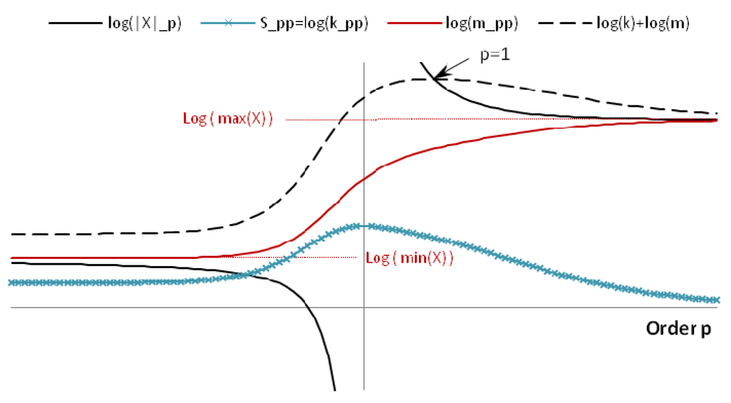
Figure 1.
Typical plot for , and in log scale.
3. An Axiomatic Approach to the Generalized Entropies and Means
In order to simplify the conceptual underpinnings, let us now describe the generalized entropies and means , through two simple axioms.
3.1. Axioms for the Generalized Entropy
Let be fixed real numbers obeying . Consider a map, , which maps multisets of positive real numbers into the real numbers. We call a generalized entropy of order if it obeys the following two axioms:
Entropy Axiom 1:
of a uniform multiset , , with multiplicity , equals , (where the base of the logarithm is arbitrarily chosen), i.e.,
Entropy Axiom 2:
If , the map depends only on the ratio of the multiset’s p and q norms, i.e., is some function, , of this ratio:
If , the map depends only on the ratio of the multiset’s q norm to its derivative, i.e., is some function, , of this ratio:
To see that (22b) arises in the limit from (22a) we notice that, since the logarithm is strictly monotone, (22a) is equivalent to saying that is some function of some finite number times the logarithm of the ratio of norms:
Choosing and taking the limit we obtain (22b) with .
Proposition: The two entropy axioms in (21) and (22) uniquely define and , namely as given in section 2 by (8) and (9).
Proof:
Entropy Axiom 2 implies that for any two multisets and :
Choosing forthe uniform multiset of Axiom 1, and taking the logarithm of both sides yields:
Using that , we now uniquely obtain the formulas for and given in (8) and (9), respectively. We note that the functions and are therefore:
Remarks:
- Even though is treated as an integer representing the multiplicity in Axiom 1, this condition is tacitly relaxed in Axiom 2 to include non-integer values, which we may call the effective cardinality (or effective dimensionality) of order .
- The logarithmic measure of Axiom 1 is directly connected to the celebrated Boltzmann entropy formula , where is the Boltzmann constant and is the number of the microstates in the system. The logarithmic measure is also connected to the so-called “Hartley’s measure” [11,12], which indicates the non-specificity [13] and does not require a probability distribution assumption. In Axiom 1, a multiset of equal positive numbers is all that is required. In fact, Axiom 1 encompasses the additivity and monotonicity axioms [12,13], which are equivalent to the earlier Khinchin’s axioms of additivity, maximality and expansibility [14].
- In Axiom 2, note that the p-norm definition is relaxed to include the values , which would result in the triangle inequality to be violated should the multisets be treated as vectors.
3.2. Axioms for the Generalized Mean
We define the pth moment of the multiset as:
The nomenclature “pth moment” is motivated by the fact that for the density function , where is the Dirac delta function, the pth moment is indeed:
Let be fixed real numbers obeying . Consider a map, , which maps multisets of positive real numbers into the real numbers. We call a generalized mean of order if it obeys the following two axioms:
Mean Axiom 1:
of a uniform multiset , is . Formally:
Mean Axiom 2:
If , the map depends for any multiset X only on the ratio of the multiset’s pth and qth moments, and , i.e., is some function, , of their ratio:
If , the map is a function only of the ratio:
The fact that (30b) is the limit of (30a) follows by the same reasoning as in (23).
Proposition:
The two mean axioms in (29) and (30) uniquely define , namely as given in (7) and (10).
Proof:
Axiom 2 implies for any two multisets and that:
Choosing the multiset to be the uniform multiset from (29) we obtain
We can now use that , to obtain and as given in (7) and (10), respectively. Accordingly the functions and are found to be
We have obtained axiomatizations of the generalized entropies and means which revealed, in particular, that the generalized entropies can be characterized as those entropies that cover the reference multiset case (the multiset of equal elements) and that are functions of only the ratio of the multisets’ and norms. Similarly, the axiomatization also revealed that the generalized means can be characterized as those means which cover the reference multiset case and which are functions of only the ratio of the multisets’ pth and qth moments and . We will now develop an axiomatization that links up with Section 2, yielding simultaneously a unique family of generalized entropies and means.
3.3. Unifying Axioms for Generalized Entropies and Means
We notice that, as is straightforward to verify:
This means that we can describe the generalized entropies and means also through a unifying set of axioms. To this end, let be fixed real numbers obeying . Consider maps and , which map multisets of positive real numbers into the real numbers. We call and generalized entropies and means of order respectively, if they obey the following two axioms:
Unifying Axiom 1:
and applied to a multiset of k equal elements , yield the values and , respectively.
Unifying axiom 2:
Proposition:
The maps and are unique and given by Equations (7)–(10).
Proof:
The proofs are straightforward and proceed similarly to the proofs of the propositions related to the entropy and mean axioms.
4. Properties of and
We list in this section useful properties of , and with proofs in the appendix. The definitions of , and are given by (7)–(10). We also add two plots for an example multiset in Figure 2 and Figure 3 in order to provide some numerical illustration of the properties hereunder.
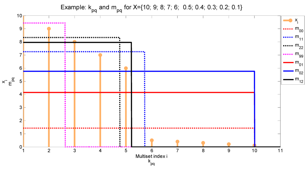
Figure 2.
Numerical example showing the multiset elements versus their index; with their corresponding mean and effective cardinality for different values of .
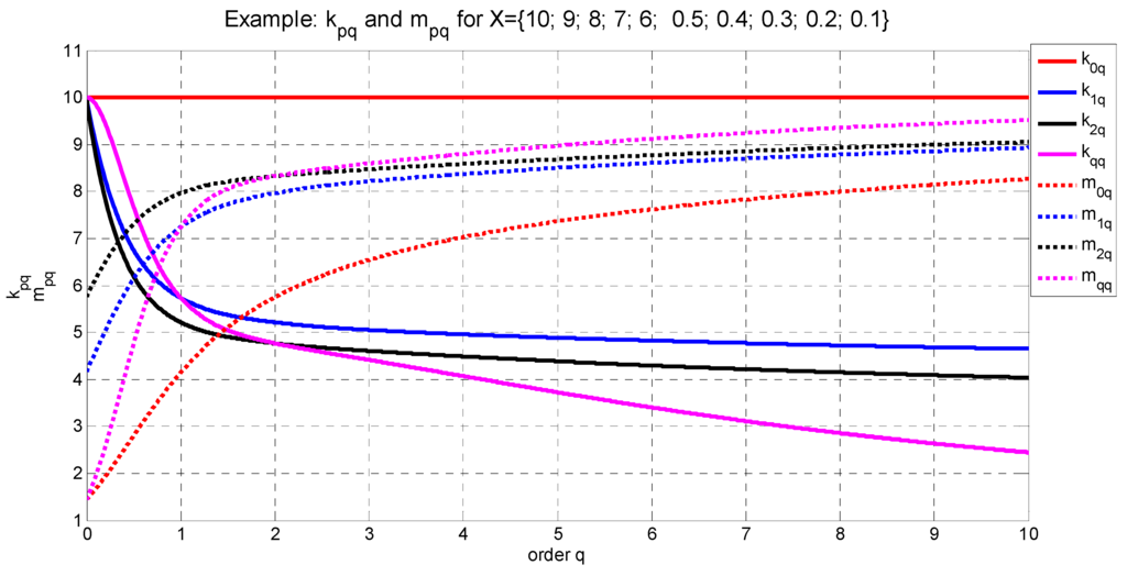
Figure 3.
Numerical example for the multiset showing its mean and effective cardinality plotted versus for fixed values of .
4.1. Scaling
Given a multiset and a constant , we have:
That is the entropy is invariant of the scaling, whereas the mean varies linearly with scaling. The proof is straightforward, based on (7).
4.2. Symmetry with Respect to the Elements of
does not depend on the order of the elements of .
4.3. Symmetry with Respect to the Order
By exchanging and in (8), we readily find that:
4.4. Sign Change of the Order
From (17), for , we obtain:
4.5. Range of
Let be the number of the non-zero elements in . Therefore:
The minimum value occurs when has exactly one non-zero element. For , the maximum value occurs when all the non-zero elements of are equal. When either or is zero, yields the maximum value, , for any distribution of , which is physically intuitive since the zeroth order renders all the non-zero multiset elements to an equal value and thus we reach the equiprobable case leading to maximum entropy. The proof of this property is in Appendix A.3.
4.6. Monotonicity of and with respect to
We have the following results for the monotonicity of and with respect to . The proofs are in Appendix B and Appendix C, respectively:
where equality holds when all the non-zero elementsare equal. Accordingly, for and , by fixing one order (say ), is always non-decreasing with respect to the other order (); whereas is non-decreasing for , non-increasing for , with a maximum value at . The result is true when switching from the symmetry Property 4.3.
Similarly, for the degenerate case , is always non-decreasing with respect to ; whereas is non-decreasing for , non-increasing for , with a maximum value at . In all cases, both the mean and entropy are invariant with respect to the order if and only if all the non-zero elements are equal.
4.7. Range of
From Property 4.6, is non-decreasing with respect to . From Table 1, we know that and . Therefore, , which is an intuitive range for a mean. This is also true in the degenerate case , i.e.,
where, as usual, equality holds when all the non-zero elements are equal.
4.8. Additivity of the Joint Multiset Entropy
For the two probability distribution multisets and , we define the joint multiset . Therefore, we have:
The proof is straightforward by using the fact that along with (7)–(10), Property 4.8 is true for both and for the degenerate case .
4.9. Sub-Additivity of the Effective Cardinality Subject to the Multiset Additive Union Operation
Let denote a multiset additive union operation [15] (page 50), e.g., . Let and be two multisets of non-negative real numbers. Moreover, let and be two positive real scaling factors of the elements of and , respectively. Then:
where the equality holds under the following condition for the value :
This property is a generalization of the effective alphabet size of two disjoint alphabets mixture as discussed in [16] (Problem 2.10). To see this, set and note that for a complete probability distribution. Accordingly, represents the effective alphabet size of corresponding to the entropy . The proof is in Appendix D.
4.10. Effective Rank of a Matrix
Let be the multiset of the singular values of a matrix . Then, . Accordingly, for general , can be viewed as a biased effective rank of corresponding to the order . From Property 4.5, we have . The minimum value occurs when has exactly one non-zero singular value (the rank of is 1). The maximum value, , is reached for any when all the non-zero singular values are equal. The effective rank can be helpful to determine, in a well-defined sense, how to view an ill-conditioned matrix, which is a full-rank from a mathematical perspective, but is effectively behaving as if possessing a lower rank. Such ill-conditioned matrices often arise in problems of oversampling or determining the degrees of freedom, where the singular values, ordered in non-increasing order by definition, exhibit some sort of “knee cut-off”, similar toin Figure 2. A biased effective rank can help to compare matrices when the knee cut-off is not sharp, thus giving more weight to the small or large singular values according to the order in a consistent manner for different matrices. An example thereof is the evaluation of the degrees of freedom of some applications such as multi-antenna systems [3,4,5,6], optical imaging systems [20], or in general any case of similar limitation to space-bandwidth product [21].
4.11. Geometrical Interpretation of and on Log Scale, with Thermodynamics Analogy
For the multiset , after taking the logarithm of both sides of (5), we obtain a simple relation between , and as in (11):
Accordingly, a secant cutting the function at and will have a slope and intercept of and , respectively, as shown in Figure 4. Based on the discussion of Section 1, (46) readily yields the following analogous expressions for a thermodynamics system described by the Boltzmann factors :
In the limiting case, when , the secant in Figure 4 becomes a tangent and we get the Gibbs–Shannon entropy at the inverse temperature . Consequently, (47) can be re-written after introducing the Boltzmann constant and using the absolute temperature as:
where is the Helmholtz free energy of the system.
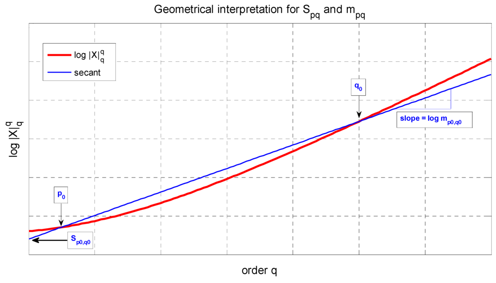
Figure 4.
A secant of versus .
5. Discussion and Conclusions
A two-parameter family of cardinalities, entropies and means has been derived for multisets of non-negative elements. Rather than starting from thermodynamic or information theoretic considerations to derive entropies and means, see e.g., [9,17,18,19], we here defined the generalized entropies and means through simple abstract axioms. There are other families of entropies in the literature (e.g., [23]), which are a generalization of Shannon entropy. The generalized entropy in this manuscript is shown to preserve the additivity (Property 4.8), which is not the case with the generalized entropies based on Tsallis non-additive entropy as in [23].
Our first two axiomatizations treat the generalized entropies and means separately. It revealed that the generalized entropies are exactly those entropies that are functions of only the ratio of the multisets’ and norms. It also revealed that the generalized means are exactly those means that are functions only of the ratio of the multisets’ pth and qth moments, and . Subsequently, our unifying axiomatization characterized the generalized entropies and means together. This showed that if two multisets have exactly the same and norms, then they share the same generalized entropy and mean.
We presented several key features of the new families of generalized entropies and means, for example, that the family of generalized entropies contains and generalizes the Rényi family of entropies, of which the Shannon entropy is a special case, thus including some of the desiderata for entropies [22]. We also showed the monotonicity with respect to , extreme values, symmetry with respect to , and additivity preservation. The effective cardinality measures the distribution uniformity of the multiset elements in the sense of the p- and q-norm equivalence to a reference flat multiset. From an information theory perspective, and represent a two-parameter entropy of order and its corresponding effective alphabet size, respectively, when a probability distribution is constructed after proper normalization of the multiset elements. Furthermore, we recall that knowing the and norms of a multiset is to know the multiset’s pth and qth moments. Our findings here therefore imply that knowledge of a multiset’s pth and qth moments is exactly enough information to deduce the multiset’s (p,q) entropy and (p,q) mean. Further, knowledge of sufficiently many moments of a multiset can be sufficient to reconstruct the multiset. Conversely, it should be interesting to examine how many (p,q)-entropies and/or (p,q)-means are required to completely determine the multiset.
Regarding the thermodynamic interpretation, we noticed that to require that the and norms of multisets coincide is mathematically equivalent to requiring that the two partition functions of two thermodynamic systems coincide at two temperatures. This in turn is equivalent to requiring that the Helmholtz free energy of the two thermodynamic systems coincide at two temperatures. The Helmholtz free energy represents the maximum mechanical work that can be extracted from a thermodynamic system under certain idealized circumstances. This suggests that there perhaps exists a thermodynamic interpretation of the generalized entropies and means in terms of the extractability of mechanical work. In this case, the fact that the generalized entropies and means depend on two rather than one temperature could be related to the fact that the maximum efficiency of a heat engine, obtained in Carnot cycles, is a function of two temperatures. We did show that in the limiting case, when the two temperatures become the same, one recovers the usual Boltzmann factor weighted mean energy as well as the usual Shannon/von Neumann entropy.
Acknowledgments
The authors gratefully acknowledge the research support by the Canada Research Chair, Discovery and Postdoctoral fellowship programs of the Natural Sciences and Engineering Research Council of Canada (NSERC).The first author is grateful for the kind hospitality at the department of Applied Mathematics at the University of Waterloo during the course of this research.
References
- Rényi, A. On the foundations of information theory. Rev. Int. Stat. Inst. 1965, 33, 1–14. [Google Scholar] [CrossRef]
- Beck, C. Generalized information and entropy measures in physics. Contemp. Phys. 2009, 50, 495–510. [Google Scholar] [CrossRef]
- Poon, A.S.Y.; Brodersen, R.W.; Tse, D.N.C. Degrees of freedom in multiple-antenna channels: A signal space approach. IEEE Trans. Inform. Theor. 2005, 51, 523–536. [Google Scholar] [CrossRef]
- Migliore, M.D. On the role of the number of degrees of freedom of the field in MIMO channels. IEEE Trans. Antenn. Propag. 2006, 54, 620–628. [Google Scholar] [CrossRef]
- Elnaggar, M.S. Electromagnetic Dimensionality of Deterministic Multi-Polarization MIMO Systems. Ph.D. Thesis; University of Waterloo: Waterloo, ON, Canada, 2007. Available online: http://uwspace.uwaterloo.ca/handle/10012/3434 (accessed on 18 April 2012).
- Elnaggar, M.S.; Safavi-Naeini, S.; Chaudhuri, S.K. A novel dimensionality metric for multi-antenna systems. In Proceedings of Asia-Pacific Microwave Conference (APMC 2006), Yokohama, Japan, December 2006; pp. 242–245.
- Elnaggar, M.S.; Kempf, A. On a Generic Entropy Measure in Physics and Information. In Proceedings of the 7th International Symposium on Modeling and Optimization in Mobile, Ad Hoc, and Wireless Networks (WiOPT 2009), Seoul, Korea, June 2009.
- Beck, C.; Schlogl, F. Thermodynamics of Chaotic Systems: An Introduction; Cambridge University Press: Cambridge, UK, 1995. [Google Scholar]
- Rényi, A. On measures of entropy and information. In Proceedings of the Fourth Berkeley Symposium on Mathematics, Statistics and Probability, University of California, Berkeley, CA, USA; 1961; Volume 1, pp. 541–561. [Google Scholar]
- Aczél, J.; Forte, B.; Ng, C.T. Why the Shannon and Hartley entropies are ‘natural’. Adv. Appl. Probab. 1974, 6, 131–146. [Google Scholar] [CrossRef]
- Hartley, R.V.L. Transmission of information. Bell Syst. Tech. J. 1928, 7, 535–564. [Google Scholar] [CrossRef]
- Rényi, A. Probability Theory; North-Holland Pub. Co.: Amsterdam, The Netherlands, 1970. [Google Scholar]
- Klir, G.J.; Folger, T.A. Fuzzy Sets, Uncertainty and Information; Prentice Hall: Upper Saddle River, NJ, USA, 1988. [Google Scholar]
- Khinchin, A.I. Mathematical Foundations of Information Theory; Dover: New York, NY, USA, 1957. [Google Scholar]
- Blizard, W.D. Multiset theory. Notre Dame J. Formal Logic 1989, 30, 36–66. [Google Scholar] [CrossRef]
- Cover, T.M.; Thomas, J.A. Elements of Information Theory; John Wiley & Sons: Hoboken, NJ, USA, 1991. [Google Scholar]
- Shannon, C.E. A mathematical theory of communication. Bell Syst. Tech. J. 1948, 27, 379–423, 623–656. [Google Scholar] [CrossRef]
- Ash, R.B. Information Theory; Interscience Publishers: New York, NY, USA, 1965. [Google Scholar]
- Reza, F.M. An Introduction to Information Theory; Dover: New York, NY, USA, 1994. [Google Scholar]
- Gori, F.; Guattari, G. Shannon number and degrees of freedom of an image. Opt. Commun. 1973, 7, 163–165. [Google Scholar] [CrossRef]
- Landau, H.; Pollak, H. Prolate spheroidal wave functions, Fourier analysis and uncertainty: Part III: The dimension of the space of essentially time- and band-limited signals. Bell Syst. Tech. J. 1962, 41, 1295–1336. [Google Scholar] [CrossRef]
- Aczel, J.; Daroczy, Z. On Measures of Information and Their Characterizations; Academic Press: New York, NY, USA, 1975. [Google Scholar]
- Shigeru, F. An axiomatic characterization of a two-parameter extended relative entropy. J. Math. Phys. 2010, 51, 123302. [Google Scholar]
Appendix A. Proof of Property 4.5: Range of
A.1. Non-Increasing with Respect to p
We want to show that is non-increasing with respect to p. This is equivalent to showing that .
Therefore, for p<q. The equality occurs only when , i.e., when includes exactly one non-zero element. Note that there is a singularity for such that and . The property herein applies over the intervals and
A.2. Non-Decreasing Generalized p-Mean with Respect to p
Let be a multiset of strictly positive numbers. For p < q, we want to show that . To this end, we define , where and , i.e., have the same sign. Clearly, and thus is convex. From Jensen’s inequality,
By setting , the proof is complete. Equality holds when all are equal.
A.3. Proof of Property 4.5:
We start by proving that . From Lemma A.1, for p < q, we have . Therefore, , and have the same sign. Since , we get . Following the same steps for p > q yields the same result. Finally, when , we have . In all cases, the equality holds when includes exactly one non-zero element.
Next, we show that . From Lemma A.2, assuming both have the same sign, for p < q, we have . Taking the logarithm yields . For p > q, we obtain the same result.
When , we have:
where was used. In all cases, equality holds when all the non-zero elements of are equal.
Appendix B. Proof of Property 4.6: Monotonicity of
B.1. Non-Degenerate Case
We have . Accordingly:
where we inserted another summation index for the last two terms in the last step. Therefore:
where we have multiplied the last two terms in the second step by . Consequently:
where we have used the fact that . The equality occurs only when for every , implying that each is either zero or some fixed value .
Accordingly, after multiplying the last inequality by , we obtain:
where the equality holds when all the non-zero elements are equal.
Since p and q are assumed to have the same sign (from the condition ), we deduce that, with respect to either p or q (while fixing the other order), is non-decreasing for negative order p,q, non-increasing for positive order p,q, with a maximum value at either (note that ). is invariant to p,q if and only if all the non-zero elements are equal.
B.2. Degenerate Case
From Appendix B.1, if , then . In the limiting case, when and , and knowing from (9) that this limit exists, we readily obtain . In a similar fashion, for negative indices values , we get . In any case, the equality occurs when all the non-zero elements are equal. has a maximum value when . Accordingly:
Appendix C. Proof of Property 4.6: Monotonicity of
C.1. Non-Degenerate Case
We have from (5) . Differentiating with respect to p, we get:
Since (Property 4.5), therefore (5) confirms that as well because the norm is defined to discard any zero elements (6). From Appendix B, . Therefore:
with equality when all the non-zero elements are equal.
C.2. Degenerate Case
From (9), , accordingly:
Moreover, from (9), . Consequently, , where we used the result of Appendix B.2. Therefore, since , we get:
Appendix D. Proof of Property 4.9: Sub-Additivity of the Effective Cardinality
For , we want to show that , where . Our objective is to find a condition in terms of and that maximizes . We have:
By setting and , we obtain the following two conditions:
From (50) and (51), we have:
Accordingly, the required proportionality condition is:
From (49), we have:
Substituting from (50) in (54) yields:
where we employed (52) to obtain the second to last step. Consequently, since and cancel out in the last step, we get:
.
In order to confirm that (53) is indeed a maximizing condition of , consider the following example. Let and with multiplicity and , respectively. From the range of (Property 4.5), we know that only when all the elements are equal, i.e., when . Indeed, (53) confirms this maximizing condition and thus .
By taking the limit when , (53) becomes
and .
© 2012 by the authors; licensee MDPI, Basel, Switzerland. This article is an open access article distributed under the terms and conditions of the Creative Commons Attribution license (http://creativecommons.org/licenses/by/3.0/).