1. Introduction
During the last decades, since the early work by Curzon and Ahlborn was published [
1], most of the studies of Finite-Time Thermodynamics (FTT) have focused on steady-state energetic properties [
2,
3,
4,
5,
6,
7,
8,
9,
10]. However, it is important to notice that any thermal engine is exposed to continuous internal and external perturbations while operating. In order to have a well-designed system, it is important to analyze the effect of noisy perturbations on the stability of the system steady state. This analysis may allow us to guarantee proper dynamical behavior of the system like stability and small relaxation times, or to warn about possible failure in the performance of a thermal engine. In 2001, Santillán
et al. [
11] studied the local stability analysis of an endoreversible Curzon-Ahlborn heat engine operating under maximum power conditions. Later, Guzmán-Vargas
et al. [
12] investigated the effect of the heat transfer laws and the thermal conductances on the local stability of an endoreversible heat engine. Recently, Páez-Hernández
et al. [
13], analyzed the local stability of a non-endoreversible Curzon-Ahlborn engine taking into account the engines implicit time delays operating at maximum power regime. However, the local stability analyses described above have not considered the effect of economical aspects. Within the context of Finite-Time Thermodynamics [
2,
3,
4,
5,
7], the effect of economical aspects was early introduced by De Vos [
14] for the study of a thermo-economic model of a power plant [
15,
16,
17]. Later, and in the same direction, Sahin and Kodal [
18] studied the thermo-economics of an endoreversible heat engine in terms of the maximization of a profit function defined as the quotient of the power output and the annual investment and the full consumption costs. This thermo-economic performance analysis [
16,
17,
19] consists in maximizing a benefit function in terms of the power output and the cost involved in the performance of the power plant [
20,
21,
22,
23,
24]. The aim of this paper is to extend the local stability analysis of the Chambadal-Novikov-Curzon-Ahlborn (CNCA) heat engine model [
1,
15,
25], by considering a Newton heat transfer law as well as to analyze the effect of internal irreversibilities and economical aspects. The paper is organized as follows: In
Section 2, we present the thermo-economical analysis of a non-endoreversible CNCA heat engine. In
Section 3, we describe the local stability analysis method applied to a two-dimensional system. In
Section 4, the local stability analysis of a CNCA heat engine is presented. Finally, in
Section 5, we present our conclusions.
2. Thermo-Economic Analysis of the Steady-State Chambadal-Novikov-Curzon-Ahlborn Heat Engine
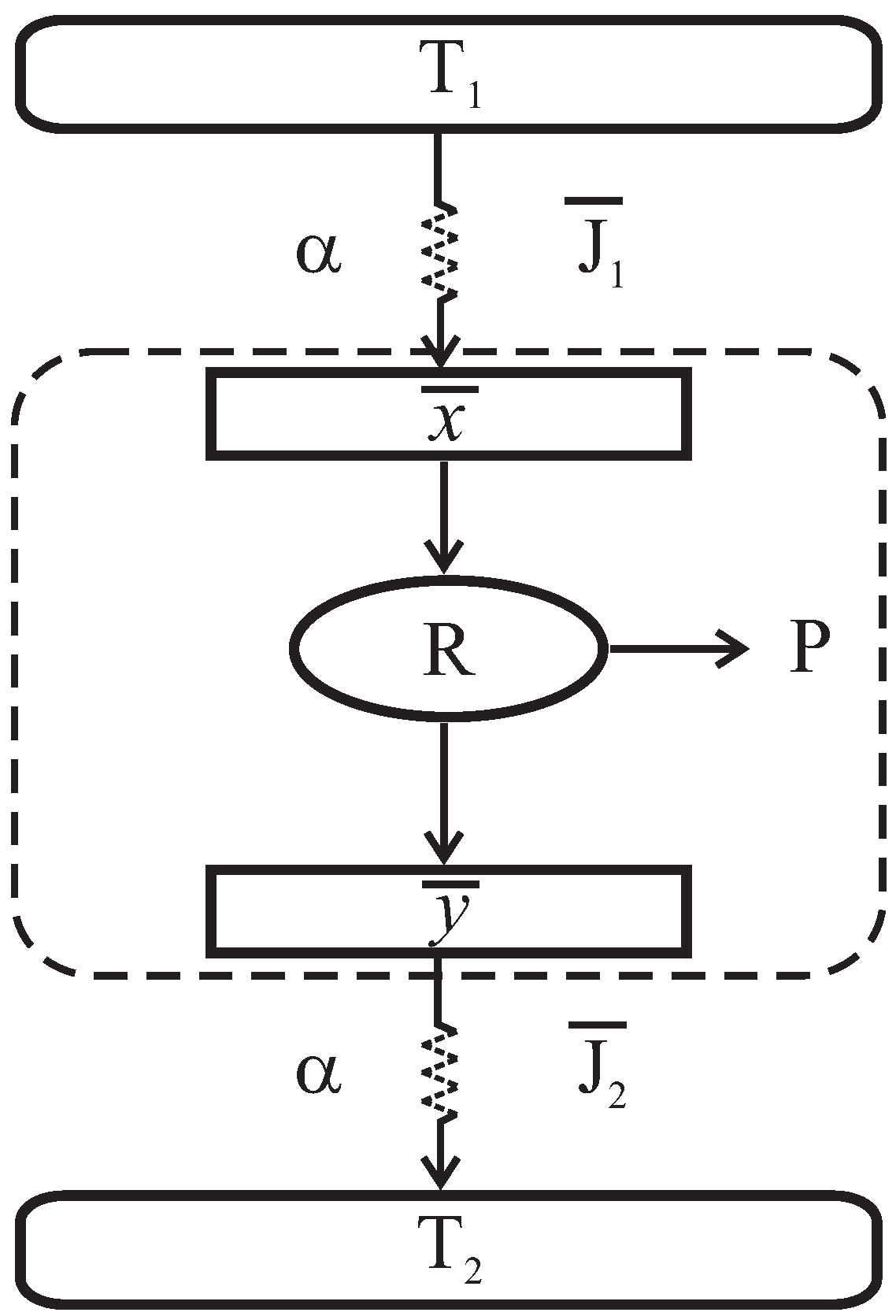
In this section, we review the thermo-economic analysis of a non-endoreversible Novikov-Curzon-Ahlborn heat engine. A schematic diagram of the CNCA engine is shown in
Figure 1. This engine consists in a Carnot-like thermal engine that works in irreversible cycles and exchanges heat with external thermal reservoirs at temperatures
and
(
). In the steady state, the temperatures of the Carnot-like cycle isothermal branches are
and
, here overbars are used to indicate the corresponding steady-state values. The steady-state heat flows between thermal reservoirs and working fluid
and
are also show in
Figure 1.
Figure 1.
Schematic representation of a non-endoreversible Curzon-Ahlborn engine.
Figure 1.
Schematic representation of a non-endoreversible Curzon-Ahlborn engine.
By applying the Clausius theorem and using the fact that the inner Carnot-like engine works in irreversible cycles, we get the following inequality
this expression can be transformed into an equality by introducing a parameter R, leading to
The parameter
R, which in principle is within the interval
(
corresponds to the endoreversible limit), can be seen as a measure of the departure from the endoreversible regime [
26,
27,
28]. If we assume that the heat flows from
to
and from
to
are of the Newton type, then
where
α is the thermal conductance. For simplicity of calculations, we have assumed that the heat exchanges take place in conductors with the same thermal conductance
α. The systems steady-state power output and the efficiency can be defined as
and
By combining Equations (
2), (
4) and (
6), we can write
and
as
where
. De Vos thermo-economical analysis considers a profit function
, which is maximized [
14]. This profit function is given by the quotient of the power output
and the total cost involved in the performance of the power plant
,
In his study, De Vos assumed that the running costs of the plant consist in two parts: a capital cost which is proportional to the investment and, therefore, to the size of the plant and, a fuel cost that is proportional to the fuel consumption and, therefore, to the heat input rate. Assuming that is an appropriate measure for the size of the plant, the running cost of the plant exploitation is defined as [
14]
where the proportionality constants
a and
b have units of
,
and
is the maximum heat that can be extracted from the heat reservoir without supplying work (see
Figure 1). By using Equations (
4), (
6), (
7), (
9) and (
10), the profit function can be written as,
If we calculate the derivative of
with respect to
, we can determine the efficiency that maximizes
by
[
29], and then we obtain
For
the result for the efficiency previously obtained by De Vos is recovered [
14,
30,
31]. Besides, when
, we obtain
, which was previously obtained by Wu and Kiang [
26], and by Arias-Hernández
et al. [
32]. Now, we consider the fractional fuel cost defined by [
14]
that is, the ratio of the fuel cost and the total cost of the plant [
14]. This parameter is related to several energy resources, taking into account energy sources where the investment is the preponderant cost (
) up to energy sources where the fuel is the predominant cost (
). This new parameter allows the efficiency and the power output to be expressed as
and
Equations (
14) and (
15) represent the steady-state efficiency
and power output
respectively. They are functions of
τ,
f and
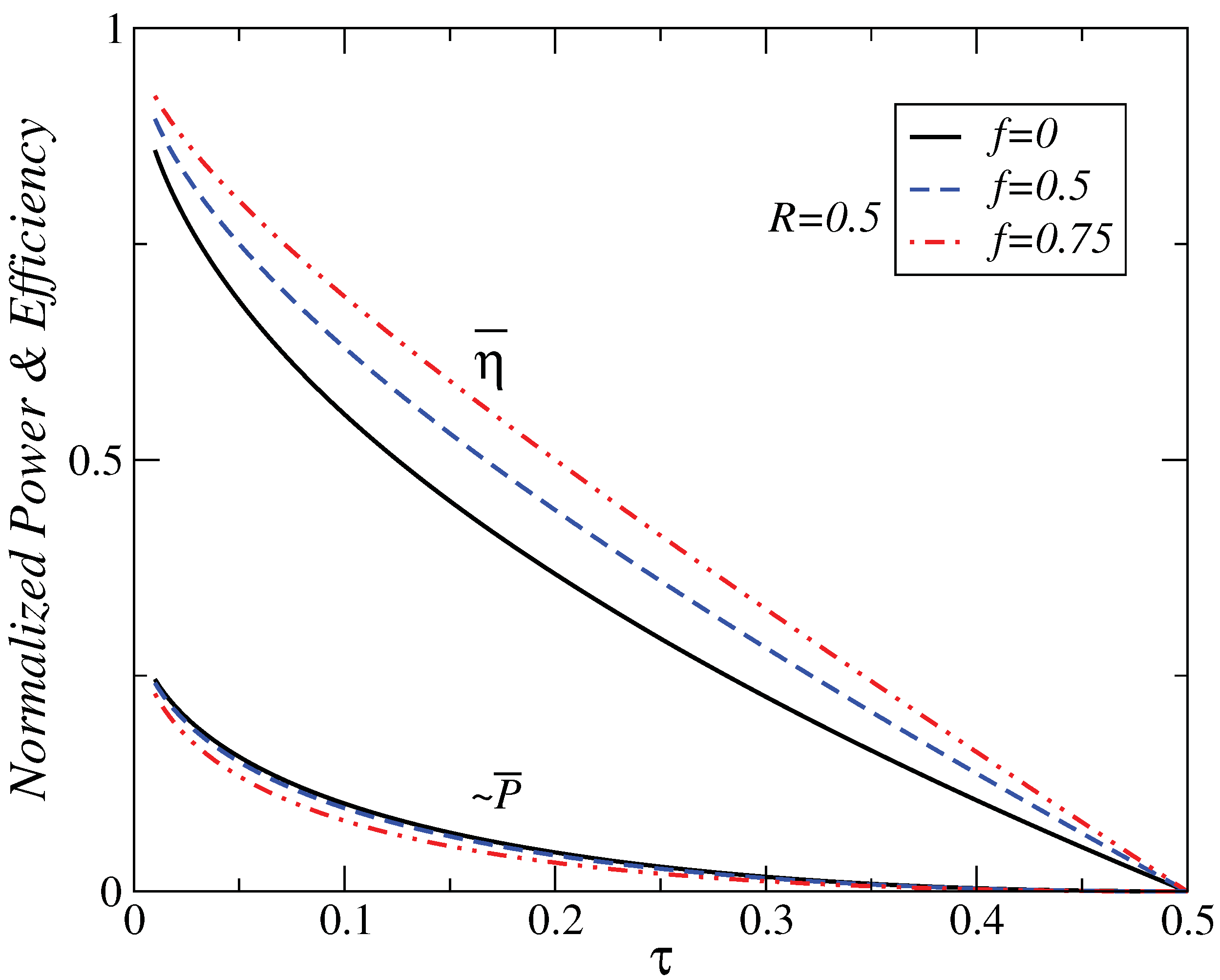
R for a non-endoreversible CNCA engine working under the maximum-profit regime. It is straightforward to show that both
and
are decreasing functions of
τ for every fixed value of
R, as we can see in
Figure 2.
Figure 2.
Plots of normalized power output ( ) and efficiency () versus τ, for different values of the fractional fuel cost.
Figure 2.
Plots of normalized power output ( ) and efficiency () versus τ, for different values of the fractional fuel cost.
3. Linearization and Stability Analysis
In this section we present a brief description of the local stability analysis for a two-dimensional system [
33]. Consider the following dynamical system,
and
Let
be a fixed point such that
and
. Consider a small perturbation around this fixed point and write
and
, where
and
are small perturbations from the corresponding fixed point values. By substituting into Equations (
16) and (
17), expanding
and
in a Taylor series, and using the fact that
and
are small to neglect quadratic terms, the following equations are obtained for the perturbations,
where
;
;
and
. Equation (
18) is a linear system of differential equations. Thus, we assume that the general solution of the system is of the form,
with
and
. Substitution of solution
into Equation (
18) yields to the following eigenvalue equation,
where
A is the matrix given by the first term in the right-hand side of Equation (
18). The eigenvalues of this equation are the roots of the characteristic equation,
If
and
are solutions of Equation (
21), the general solution of the system is
where
and
are arbitrary constants and
and
are the eigenvectors corresponding to
and
, respectively. To determine
and
we use again Equation (
20) for each eigenvalue. Information about the stability of the system can be obtained from the value of the eigenvalues
and
. In general,
and
are complex numbers. If both
and
have negative real parts, the fixed point is stable. Moreover, if both eigenvalues are real and negative, the perturbations decay exponentially [
33]. In this last case, it is possible to identify characteristic time scales for each eigendirection as
and
4. Local Stability Analysis
Following Santillán
et al. [
11], and assuming that the working fluid at the isothermal branches
x and
y are not real heat reservoirs but macroscopic objects with heat capacity
C, the internal temperatures
x and
y (see
Figure 1) change according to the following differential equations
and
where
and
are the heat flows described in
Figure 1. According to the non-endoreversibility hypothesis,
and
are given by
and
On the other hand, we can use Equations (
6) and (
14) to construct an expression which relates the internal variables
and
, to the external temperatures
and
, given by
In a similar way to Equation (
29), by using Equations (
7) and (
14), we can obtain an expression for
The corresponding steady-state values of
and
as function of
and
at maximum-profit function are obtained by substituting Equation (
14) into Equations (
7) and (
8), respectively
and
We can observe from Equations (
29)–(
32) that for the case
and
, the results previously obtained by Santillán
et al. [
11] and Guzmán-Vargas
et al. [
12] are recovered. Finally, by substituting Equations (
29) and (
30) into Equation (
15), the steady-state power output can be expressed as
where
By using the assumption [
11,
12] that out of the steady state but not too far away, the power output of a Curzon-Ahlborn heat engine depends on
x and
y in the same way that it depends on
and
at the steady-state (
), that is, this assumption is applicable only in the vicinity of the steady state, we can write the dynamical equations for
x and
y as follows
and
To analyze the system stability near the steady state, we proceed following the steps described in the previous sections. After solving the corresponding eigenvalue equation, we find that both eigenvalues (
and
) are function of
α,
C,
τ,
f and
R. The final expression and the algebraic details are not shown because they are quite lengthy and can be easily reproduced with the help of a symbolic algebra package. Specifically, our calculations show that both eigenvalues are real and negative, with
, and then
, where
,
correspond to the slow and fast eigendirection, respectively. Thus, the steady state is stable because any perturbation would be decay exponentially. The expressions of the eigenvalues when
are consistent with those previously reported in [
11,
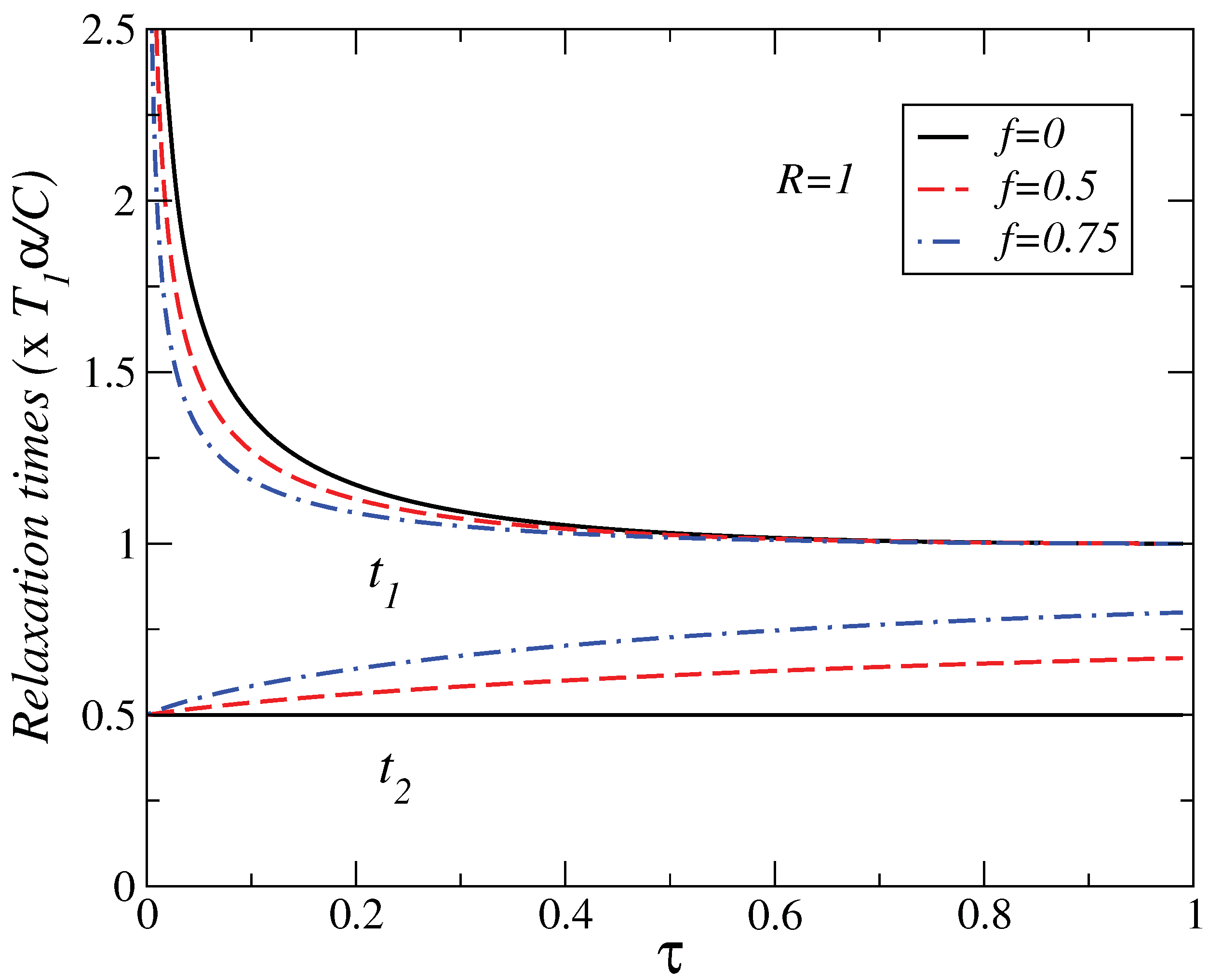
12]. In
Figure 3, the relaxation times are plotted against
τ for different values of fractional fuel cost
f, for a fixed value of
R (
), that is, the endoreversible case. We observe that
is a decreasing function of
τ. This relaxation time decreases as the fuel cost increases, indicating a faster decay along this eigendirection as
.
Figure 3.
Plot of relaxation times versus τ for several values of the fractional fuel cost f in the endoreversible case ().
Figure 3.
Plot of relaxation times versus τ for several values of the fractional fuel cost f in the endoreversible case ().
For
, we observe that this relaxation time remains constant as
τ increases for
. As the fractional fuel cost
f increases,
slightly increases too. We notice that in the limit
, both relaxation times tend to be closer each other, indicating that the stability is preserved for values within the interval
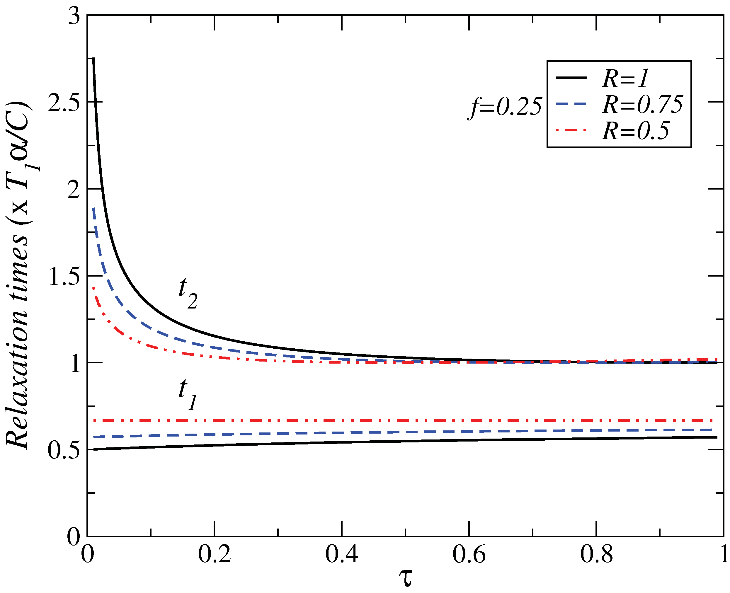
. In
Figure 4 we also show the relaxation times as a function of
τ, for several values of the parameter
R, for a fixed value of the fractional fuel cost
f. As in
Figure 3,
is a decreasing function of
τ. We observe that
remains almost constant and slightly increases when the irreversibility parameter changes. From the findings of
Figure 3 and
Figure 4, we can conclude that the system is stable for
. We remark that as the fractional fuel cost
f increases,
decreases whereas
varies smoothly, for a given value of
R. Likewise, for a given value of
f, as the irreversibility parameter
R decreases,
decreases whereas
increases. Additionally, in
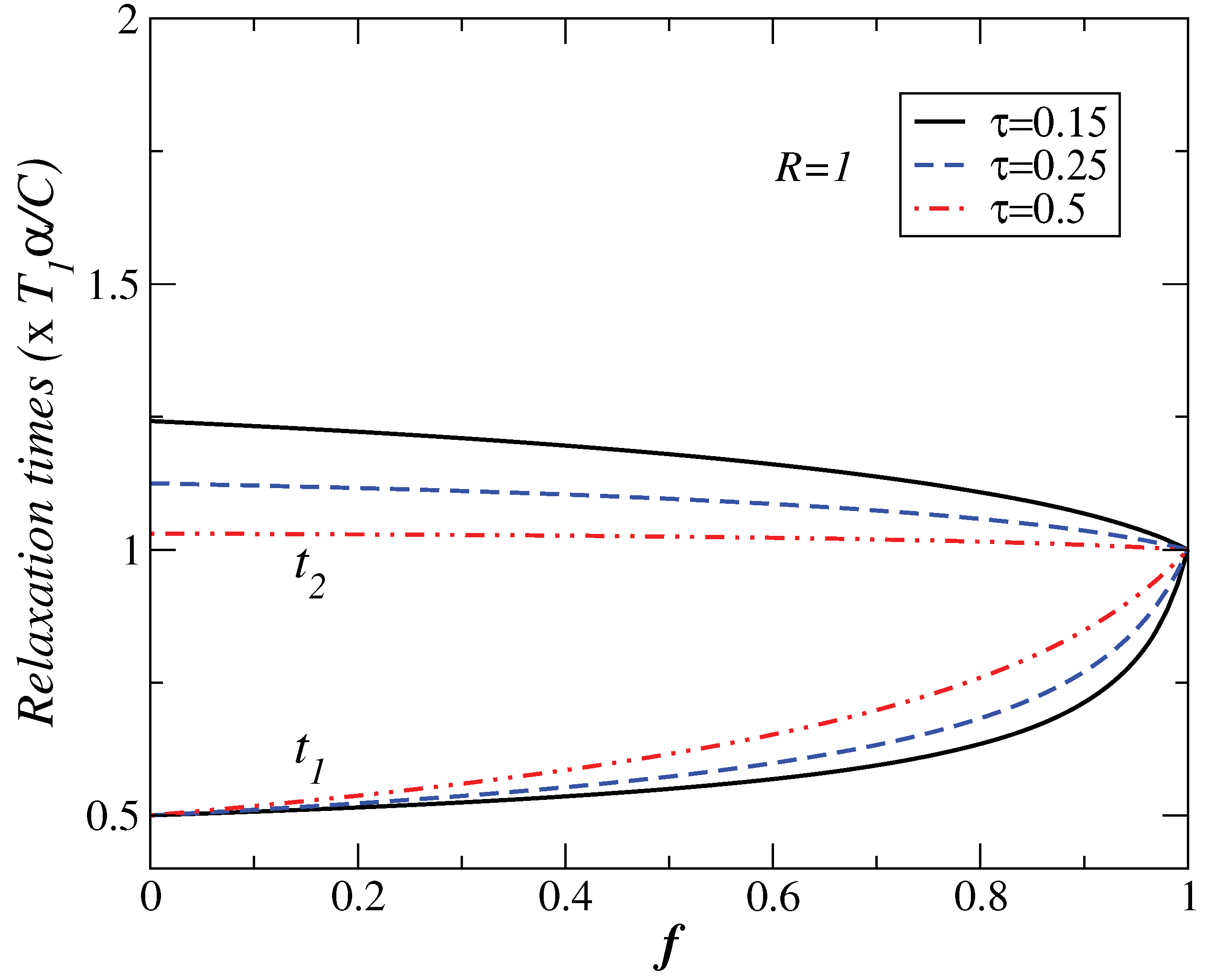
Figure 5 we show the relaxation times
versus fuel fractional cost for several values of
τ. We can see, in this case, how the fast (slow) relaxation time slightly increases (decreases) as
f changes from 0 to 1. It is important to notice that the optimal efficiency smoothly increases as
f moves from 0 to 1, and we have seen that the stability is preserved for variations of
f in the same range. We also remark that the power output and the efficiency depend on
τ for the cases analyzed here, and both energetic quantities are decreasing functions of this parameter, that is, the systems stability moves in the opposite direction to that of the steady state
P and
η as
τ varies.
Figure 4.
Plot of relaxation times versus τ for several values of the endoreversibility parameter R and a value of the fractional fuel cost.
Figure 4.
Plot of relaxation times versus τ for several values of the endoreversibility parameter R and a value of the fractional fuel cost.
Figure 5.
Relaxation times versus f for several values of τ in the endoreversible case.
Figure 5.
Relaxation times versus f for several values of τ in the endoreversible case.
