Review

Using Quantum Computers for Quantum Simulation

1
School of Physics and Astronomy, University of Leeds, Woodhouse Lane, Leeds LS2 9JT, UK
2
National Institute of Informatics, 2-1-2 Hitotsubashi, Chiyoda-ku, Tokyo, 101-8430, Japan
3
NTT Basic Research Laboratories, NTT Corporation, 3-1 Morinosato-Wakamiya, Atsugi-shi, Kanagawa-ken 243-0198, Japan
*
Author to whom correspondence should be addressed.
Entropy 2010, 12(11), 2268-2307; https://doi.org/10.3390/e12112268
Submission received: 2 October 2010 / Revised: 2 November 2010 / Accepted: 10 November 2010 / Published: 15 November 2010
(This article belongs to the Collection Quantum Information)

Abstract

:
Numerical simulation of quantum systems is crucial to further our understanding of natural phenomena. Many systems of key interest and importance, in areas such as superconducting materials and quantum chemistry, are thought to be described by models which we cannot solve with sufficient accuracy, neither analytically nor numerically with classical computers. Using a quantum computer to simulate such quantum systems has been viewed as a key application of quantum computation from the very beginning of the field in the 1980s. Moreover, useful results beyond the reach of classical computation are expected to be accessible with fewer than a hundred qubits, making quantum simulation potentially one of the earliest practical applications of quantum computers. In this paper we survey the theoretical and experimental development of quantum simulation using quantum computers, from the first ideas to the intense research efforts currently underway.

Graphical Abstract

1. Introduction

The role of numerical simulation in science is to work out in detail what our mathematical models of physical systems predict. When the models become too difficult to solve by analytical techniques, or details are required for specific values of parameters, numerical computation can often fill the gap. This is only a practical option if the calculations required can be done efficiently with the resources available. As most computational scientists know well, many calculations we would like to do require more computational power than we have. Running out of computational power is nearly ubiquitous whatever you are working on, but for those working on quantum systems this happens for rather small system sizes. Consequently, there are significant open problems in important areas, such as high temperature superconductivity, where progress is slow because we cannot adequately test our models or use them to make predictions.
Simulating a fully general quantum system on a classical computer is possible only for very small systems, because of the exponential scaling of the Hilbert space with the size of the quantum system. To appreciate just how quickly this takes us beyond reasonable computational resources, consider the classical memory required to store a fully general state | ψ n of n qubits (two-state quantum systems). The Hilbert space for n qubits is spanned by 2 n orthogonal states, labeled | j with 0 j < 2 n . The n qubits can be in a superposition of all of them in different proportions,
| ψ n = j = 0 2 n - 1 c j | j
To store this description of the state in a classical computer, we need to store all of the complex numbers { c j } . Each requires two floating point numbers (real and imaginary parts). Using 32 bits (4 bytes) for each floating point number, a quantum state of n = 27 qubits will require 1 Gbyte of memory—a new desktop computer in 2010 probably has around 2 to 4 Gbyte of memory in total. Each additional qubit doubles the memory, so 37 qubits would need a Terabyte of memory—a new desktop computer in 2010 probably has a hard disk of this size. The time that would be required to perform any useful calculation on this size of data is actually what becomes the limiting factor. One of the largest simulations of qubits on record [1] computed the evolution of 36 qubits in a quantum register using one Terabyte of memory, with multiple computers for the processing. Simulating more than 40 qubits in a fully general superposition state is thus well beyond our current capabilities. Computational physicists can handle larger systems if the model restricts the dynamics to only part of the full Hilbert space. Appropriately designed methods then allow larger classical simulations to be performed [2]. However, any model is only as good as its assumptions, and capping the size of the accessible part of the Hilbert space below 2 36 orthogonal states for all system sizes is a severe restriction.
The genius of Feynman in 1982 was to come up with an idea for how to circumvent the difficulties of simulating quantum systems classically [3]. The enormous Hilbert space of a general quantum state can be encoded and stored efficiently on a quantum computer using the superpositions it has naturally. This was the original inspiration for quantum computation, independently proposed also by Deutsch [4] a few years later. The low threshold for useful quantum simulations, of upwards of 36 or so qubits, means it is widely expected to be one of the first practical applications of a quantum computer. Compared to the millions of qubits needed for useful instances of other quantum algorithms, such as Shor’s algorithm for factoring [5], this is a realistic goal for current experimental research to work towards. We will consider the experimental challenges in the latter sections of this review, after we have laid out the theoretical requirements.
Although a quantum computer can efficiently store the quantum state under study, it is not a “drop in” replacement for a classical computer as far as the methods and results are concerned. A classical simulation of a quantum system gives us access to the full quantum state, i.e., all the 2 n complex numbers { c j } in Equation (1). A quantum computer storing the same quantum state can in principle tell us no more than whether one of the { c j } is non-zero, if we directly measure the quantum state in the computational basis. As with all types of quantum algorithm, an extra step is required in the processing to concentrate the information we want into the register for the final measurement. Particularly for quantum simulation, amassing enough useful information also typically requires a significant number of repetitions of the simulation. Classical simulations of quantum systems are usually “strong simulations” [6,7] which provide the whole probability distribution, and we often need at least a significant part of this, e.g., for correlation functions, from a quantum simulation. If we ask only for sampling from the probability distribution, a “weak simulation”, then a wider class of quantum computations can be simulated efficiently classically, but may require repetition to provide useful results, just as the quantum computation would. Clearly, it is only worth using a quantum computer when neither strong nor weak simulation can be performed efficiently classically, and these are the cases we are interested in for this review.
As with all quantum algorithms, the three main steps, initialization, quantum processing, and data extraction (measurement) must all be performed efficiently to obtain a computation that is efficient overall. Efficient in this context will be taken to mean using resources that scale polynomially in the size of the problem, although this isn’t always a reliable guide to what can be achieved in practice. For many quantum algorithms, the initial state of the computer is a simple and easy to prepare state, such as all qubits set to zero. However, for a typical quantum simulation, the initial state we want is often an unknown state that we are trying to find or characterise, such as the lowest energy state. The special techniques required to deal with this are discussed in Section 4. The second step is usually the time evolution of the Hamiltonian. Classical simulations use a wide variety of methods, depending on the model being used, and the information being calculated. The same is true for quantum simulation, although the diversity is less developed, since we don’t have the possibility to actually use the proposed methods on real problems yet and refine through practice. Significant inovation in classical simulation methods arose as a response to practical problems encountered when theoretical methods were put to the test, and we can expect the same to happen with quantum simulation. The main approach to time evolution using a universal quantum computer is described in Section 2.1, in which the Lloyd method for evolving the Hamiltonian using Trotterization is described. In Section 5, further techniques are described, including the quantum version of the pseudo-spectral method that converts between position and momentum space to evaluate different terms in the Hamiltonian using the simplest representation for each, and quantum lattice gases, which can be used as a general differential equation solver in the same way that classical lattice gas and lattice Boltzmann methods are applied. It is also possible to take a direct approach, in which the Hamiltonian of the quantum simulator is controlled in such a way that it behaves like the one under study—an idea already well established in the Nuclear Magnetic Resonance (NMR) community. The relevant theory is covered in Section 2.3. The final step is data extraction. Of course, data extraction methods are dictated by what we want to calculate, and this in turn affects the design of the whole algorithm, which is why it is most naturally discussed before initialization, in Section 3.
For classical simulation, we rarely use anything other than standard digital computers today. Whatever the problem, we map it onto the registers and standard gate operations available in a commercial computer (with the help of high level programming languages and compilers). The same approach to quantum simulation makes use of the quantum computer architectures proposed for universal quantum computation. The seminal work of Lloyd [8] gives the conditions under which quantum simulations can be performed efficiently on a universal quantum computer. The subsequent development of quantum simulation algorithms for general purpose quantum computers accounts for a major fraction of the theoretical work in quantum simulation. However, special purpose computational modules are still used for classical applications in many areas, such as fast real time control of experimental equipment, or video rendering on graphics cards to control displays, or even mundane tasks such as controlling a toaster, or in a digital alarm clock. A similar approach can also be used for quantum simulation. A quantum simulator is a device which is designed to simulate a particular Hamiltonian, and it may not be capable of universal quantum computation. Nonetheless, a special purpose quantum simulator could still be fast and efficient for the particular simulation it is built for. This would allow a useful device to be constructed before we have the technology for universal quantum computers capable of the same computation. This is thus a very active area of current research. We describe a selection of these in the experimental Section 8 to Section 10, which begins with its own overview in Section 7.
While we deal here strictly with quantum simulation of quantum systems, some of the methods described here, such as lattice gas automata, are applicable to a wider class of problems, which will be mentioned as appropriate. A short review such as this must necessarily be brief and selective in the material covered from this broad and active field of research. In particular, the development of Hamiltonian simulation applied to quantum algorithms begun by the seminal work of Aharonov and Ta-Shma [9]—which is worthy of a review in itself—is discussed only where there are implications for practical applications. Where choices had to be made, the focus has been on relevance to practical implementation for solving real problems, and reference has been made to more detailed reviews of specific topics, where they already exist. The pace of development in this exciting field is such that it will in any case be important to refer to more recent publications to obtain a fully up to date picture of what has been achieved.

2. Universal Quantum Simulation

The core processing task in quantum simulation will usually be the time evolution of a quantum system under a given Hamiltonian,
| Ψ ( t ) = exp ( i H ^ t ) | Ψ ( 0 )
Given the initial state | Ψ ( 0 ) and the Hamiltonian H ^ , which may itself be time dependent, calculate the state of the system | Ψ ( t ) at time t. In many cases it is the properties of a system governed by the particular Hamiltonian that are being sought, and pure quantum evolution is sufficient. For open quantum systems where coupling to another system or environment plays a role, the appropriate master equation will be used instead. In this section we will explore how accomplish the time evolution of a Hamiltonian efficiently, thereby explaining the basic theory underlying quantum simulation.

2.1. Lloyd’s Method

Feynman’s seminal ideas [3] from 1982 were fleshed out by Lloyd in 1996, in his paper on universal quantum simulators [8]. While a quantum computer can clearly store the quantum state efficiently compared with a classical computer, this is only half the problem. It is also crucial that the computation on this superposition state can be performed efficiently, the more so because classically we actually run out of computational power before we run out of memory to store the state. Lloyd notes that simply by turning on and off the correct sequence of Hamiltonians, a system can be made to evolve according to any unitary operator. By decomposing the unitary operator into a sequence of standard quantum gates, Vartiainen et al. [10] provide a method for doing this with a gate model quantum computer. However, an arbitrary unitary operator requires exponentially many parameters to specify it, so we don’t get an efficient algorithm overall. A unitary operator with an exponential number of parameters requires exponential resources to simulate it in both the quantum and classical cases. Fortunately, (as Feynman had envisaged), any system that is consistent with special and general relativity evolves according to local interactions. All Hamiltonian evolutions H ^ with only local interactions can be written in the form
H ^ = j = 1 n H ^ j
where each of the n local Hamiltonians H ^ j acts on a limited space containing at most of the total of N variables. By “local” we only require that remains fixed as N increases, we don’t require that the variables are actually spatially localised, allowing efficient simulation for many non-relativistic models with long-range interactions. The number of possible distinct terms H ^ j in the decomposition of H ^ is given by the binomial coefficient N < N / ! . Thus n < N / ! is polynomial in N. This is a generous upper bound in many practical cases: for Hamiltonians in which each system interacts with at most nearest neighbours, n N .
In the same way that classical simulation of the time evolution of dynamical systems is often performed, the total simulation time t can be divided up into τ small discrete steps. Each step is approximated using a Trotter-Suzuki [11,12] formula,
exp { i H ^ t } = exp { i H ^ 1 t / τ } exp { i H ^ n t / τ } τ + j > j [ H j , H j ] t 2 / 2 τ + higher order terms
The higher order term of order k is bounded by τ | | H ^ t / τ | | sup k / k ! , where | | A ^ | | s u p is the supremum, or maximum expectation value, of the operator A ^ over the states of interest. The total error is less than | | τ { exp ( i H ^ t / τ ) - 1 - i H ^ t / τ } | | sup if just the first term in Equation (4) is used to approximate exp ( i H ^ t ) . By taking τ to be sufficiently large the error can be made as small as required. For a given error ϵ, from the second term in Equation (4) we have ϵ t 2 / τ . A first order Trotter-Suzuki simulation thus requires τ t 2 / ϵ .
Now we can check that the simulation scales efficiently in the number of operations required. The size of the most general Hamiltonian H ^ j between variables depends on the dimensions of the individual variables but will be bounded by a maximum size g. The Hamiltonians H ^ and { H ^ j } can be time dependent so long as g remains fixed. Simulating exp { i H ^ j t / τ } requires g j 2 operations where g j g is the dimension of the variables involved in H ^ j . In Equation (4), each local operator H ^ j is simulated τ times. Therefore, the total number of operations required for simulating exp { i H ^ t } is bounded by τ n g 2 . Using τ t 2 / ϵ , the number of operations O p Lloyd is given by
O p Lloyd t 2 n g 2 / ϵ
The only dependence on the system size N is in n, and we already determined that n is polynomial in N, so the number of operations is indeed efficient by the criterion of polynomial scaling in the problem size.
The simulation method provided by Lloyd that we just described is straightforward but very general. Lloyd laid the groundwork for subsequent quantum simulation development, by providing conditions (local Hamiltonians) under which it will be possible in theory to carry out efficient quantum simulation, and describing an explicit method for doing this. After some further consideration of the way the errors scale, the remainder of this section elaborates on exactly which Hamiltonians H ^ q in a quantum simulator can efficiently simulate which other Hamiltonians H ^ j in the system under study.

2.2. Errors and Efficiency

Although Lloyd [8] explicitly notes that to keep the total error below ϵ, each operation must have error less than ϵ / ( τ n g 2 ) where n = poly ( N ) , he does not discuss the implications of this scaling as an inverse polynomial in N. For digital computation, we can improve the accuracy of our results by increasing the number of bits of precision we use. In turn, this increases the number of elementary (bitwise) operations required to process the data. To keep the errors below a chosen ϵ by the end of the computation, we must have log 2 ( 1 / ϵ ) accurate bits in our output register. The resources required to achieve this in an efficient computation scale polynomially in log 2 ( 1 / ϵ ) . In contrast, as already noted in Equation (5), the resources required for quantum simulation are proportional to t 2 n g 2 / ϵ , so the dependence on ϵ is inverse, rather than log inverse.
The consequences of this were first discussed by Brown et al. [13], who point out that all the work on error correction for quantum computation assumes a logarithmic scaling of errors with the size of the computation, and they experimentally verify that the errors do indeed scale inversely for an NMR implementation of quantum simulation. To correct these errors thus requires exponentially more operations for quantum simulation than for a typical (binary encoded) quantum computation of similar size and precision. This is potentially a major issue, once quantum simulations reach large enough sizes to solve useful problems. The time efficiency of the computation for any quantum simulation method will be worsened due to the error correction overheads. This problem is mitigated somewhat because we may not actually need such high precision for quantum simulation as we do for calculations involving integers, for example. However, Clark et al. [14] conducted a resource analysis for a quantum simulation to find the ground state energy of the transverse Ising model performed on a circuit model quantum computer. They found that, even with modest precision, error correction requirements result in unfeasibly long simulations for systems that would be possible to simulate if error correction weren’t necessary. One of the main reasons for this is the use of Trotterization, which entails a large number of steps τ each composed of many operations with associated imperfections requiring error correction.
Another consequence of the polynomial scaling of the errors, explored by Kendon et al. [15], is that analogue (continuous variable) quantum computers may be equally suitable for quantum simulation, since they have this same error scaling for any computation they perform. This means they are usually considered only for small processing tasks as part of quantum communications networks, where the poor scaling is less of a problem. As Lloyd notes [8], the same methods as for discrete systems generalise directly onto continuous variable systems and Hamiltonians.
On the other hand, this analysis doesn’t include potential savings that can be made when implementing the Lloyd method, such as by using parallel processing to compute simultaneously the terms in Equation (3) that commute. The errors due to decoherence can also be exploited to simulate the effects of noise on the system being studied, see Section 5.4. Nonetheless, the unfavorable scaling of the error correction requirements with system size in quantum simulation remains an under-appreciated issue for all implementation methods.

2.3. Universal Hamiltonians

Once Lloyd had shown that quantum simulation can be done efficiently overall, attention turned to the explicit forms of the Hamiltonians, both the { H ^ j } in the system to be simulated, and the { H ^ q } available in the quantum computer. Since universal quantum computation amounts to being able to implement any unitary operation on the register of the quantum computer, this includes quantum simulation as a special case, i.e., the unitary operations derived from local Hamiltonians. Universal quantum computation is thus sufficient for quantum simulation, but this leaves open the possibility that universal quantum simulation could be performed equally efficiently with less powerful resources. There is also the important question of how much the efficiency can be improved by exploiting the { H ^ q } in the quantum computer directly rather than through standard quantum gates.
The natural idea that mapping directly between the { H ^ j } and the { H ^ q } should be the most efficient way to do quantum simulation resulted in a decade of research that has answered almost all the theoretical questions one can ask about exactly which Hamiltonians can simulate which other Hamiltonians, and how efficiently. The physically-motivated setting for much of this work is a quantum computer with a single, fixed interaction between the qubits, that can be turned on and off but not otherwise varied, along with arbitrary local control operations on each individual qubit. This is a reasonable abstraction of a typical quantum computer architecture: controlled interactions between qubits are usually hard and/or slow compared with rotating individual qubits. Since most non-trivial interaction Hamiltonians can be used to do universal quantum computation, it follows they can generally simulate all others (of the same system size or smaller) as well. However, determining the optimal control sequences and resulting efficiency is computationally hard in the general case [16,17,18], which is not so practical for building actual universal quantum simulators. These results are thus important for the theoretical understanding of the interconvertability of Hamiltonians, but for actual simulator design we will need to choose Hamiltonians { H ^ q } for which the control sequences can be obtained efficiently.
Dodd et al. [19], Bremner et al. [20], and Nielsen et al. [21] characterised non-trivial Hamiltonians as entangling Hamiltonians, in which every subsystem is coupled to every other subsystem either directly or via intermediate subsystems. When the subsystems are qubits (two-state quantum systems), multi-qubit Hamiltonians involving an even number of qubits provide universal simulation, when combined with local unitary operations. Qubit Hamiltonians where the terms couple only odd numbers of qubits are universal for the simulation of one fewer logical qubits (using a special encoding) [22]. When the subsystems are qudits (quantum systems of dimension d), any two-body qudit entangling Hamiltonian is universal, and efficiently so, when combined with local unitary operators [21]. This is a useful and illuminating approach because of the fundamental role played by entanglement in quantum information processing. Entanglement can only be generated by interaction (direct or indirect) between two (or more) parties. The local unitaries and controls can thus only move the entanglement around, they cannot increase it. These results show that generating enough entanglement can be completely separated from the task of shaping the exact form of the Hamiltonian. Further work on general Hamiltonian simulation has been done by McKague et al. [23] who have shown how to conduct a multipartite simulation using just a real Hilbert space. While not of practical importance, this is significant in relation to foundational questions. It follows from their work that Bell inequalities can be violated by quantum states restricted to a real Hilbert space. Very recent work by Childs et al. [24] fills in most of the remaining gaps in our knowledge of the conditions under which two-qubit Hamiltonians are universal for approximating other Hamiltonians (equally applicable to both quantum simulation and computation). There are only three special types of two-qubit Hamiltonians that aren’t universal for simulating other two-qubit Hamiltonians, and some of these are still universal for simulating Hamiltonians on more than two qubits.

2.4. Efficient Hamiltonian Simulation

The other important question about using one Hamiltonian to simulate another is how efficiently it can be done. The Lloyd method described in Section 2.1 can be improved to bring the scaling with t down from quadratic, Equation (5), to close to linear by using higher order terms from the Trotter-Suzuki expansion [11]. This is close to optimal, because it is not possible to perform simulations in less than linear time, as Berry et al. [25] prove. They provide a formula for the optimal number k opt of higher order terms to use, trading off extra operations per step τ for less steps due to the improved accuracy of each step,
k opt = 1 2 log 5 ( n | | H ^ | | t / ϵ )
where | | H ^ | | is the spectral norm of H ^ (equal to the magnitude of the largest eigenvalue for Hermitian matrices). The corresponding optimal number of operations is bounded by
O p Berry 4 g 2 n 2 | | H ^ | | t exp 2 ln 5 ln ( n | | H ^ | | t / ϵ )
This is close to linear for large ( n | | H ^ | | t ) . Recent work by Papageorgiou and Zhang [26] improves on Berry et al.’s results, by explicitly incoporating the dependence on the norms of the largest and next largest of the H ^ j in Equation (3).
Berry et al. [25] also consider more general Hamiltonians, applicable more to quantum algorithms than quantum simulation. For a sparse Hamiltonian, i.e., with no more than a fixed number of nonzero entries in each column of its matrix representation, and a black box function which provides one of these entries when queried, they derive a bound on the number of calls to the black box function required to simulate the Hamiltonian H ^ . When | | H ^ | | is bounded by a constant, the number of calls to obtain matrix elements scales as
O ( ( log * n ) t 1 + 1 / 2 k )
where n is the number of qubits necessary to store a state from the Hilbert space on which H ^ acts, and log * n is the iterative log function, the number of times log has to be applied until the result is less than or equal to one. This is a very slowly growing function, for practical values of n it will be less than about five. This scaling is thus almost optimal, since (as already noted) sub-linear time scaling is not possible. These results apply to Hamiltonians where there is no tensor product structure, so generalise what simulations it is possible to perform efficiently. Child and Kothari [27,28] provide improved methods for sparse Hamiltonians by decomposing them into sums where the graphs corresponding to the non-zero entries are star graphs. They also prove a variety of cases where efficient simulation of non-sparse Hamiltonians is possible, using the method developed by Childs [29] to simulate Hamiltonians using quantum walks. These all involve conditions under which an efficient description of a non-sparse Hamiltonian can be exploited to simulate it. While of key importance for the development of quantum algorithms, these results don’t relate directly to simulating physical Hamiltonians.
If we want to simulate bipartite (i.e., two-body) Hamiltonians { H ^ j ( 2 ) } using only bipartite Hamiltonians { H ^ q ( 2 ) } , the control sequences can be efficiently determined [17,18,30]. Dür, Bremner and Briegel [31] provide detailed prescriptions for how to map higher-dimensional systems onto pairwise interacting qubits. They describe three techniques: using commutators between different H ^ q to build up higher order interactions; graph state encodings; and teleportation-based methods. All methods incur a cost in terms of resources and sources of errors, which they also analyse in detail. The best choice of technique will depend on the particular problem and type of quantum computer available.
The complementary problem: given two-qubit Hamiltonians, how can higher dimensional qubit Hamiltonians be approximated efficiently, was tackled by Bravyi et al. [32]. They use perturbation theory gadgets to construct the higher order interactions, which can be viewed as a reverse process to standard perturbation theory. The generic problem of -local Hamiltonians in an algorithmic setting is known to be NP-hard for finding the ground state energy, but Bravyi et al. apply extra constraints to restrict the Hamiltonians of both system and simulation to be physically realistic. Under these conditions, for many-body qubit Hamiltonians H ^ = j H ^ j ( ) with a maximum of interactions per qubit, and where each qubit appears in only a constant number of the { H ^ j ( ) } terms, Bravyi et al. show that they can be simulated using two-body qubit Hamiltonians { H ^ q ( 2 ) } with an absolute error given by n ϵ | | H ^ j ( ) | | sup ; where ϵ is the precision, | | H ^ j ( ) | | sup the largest norm of the local interactions and n is the number of qubits. For physical Hamiltonians, the ground state energy is proportional to n | | H ^ j ( ) | | , allowing an efficient approximation of the ground state energy with arbitrarily small relative error ϵ.
Two-qubit Hamiltonians { H ^ q ( 2 ) } with local operations are a natural assumption for modelling a quantum computer, but so far we have only discussed the interaction Hamiltonian. Vidal and Cirac [33] consider the role of and requirements for the local operations in more detail, by adding ancillas-mediated operations to the available set of local operations. They compare this case with that of local operations and classical communication (LOCC) only. For a two-body qubit Hamiltonian, the simulation can be done with the same time efficiency, independent of whether ancillas are used, and this allows the problem of time optimality to be solved [30]. However, for other cases using ancillas gives some extra efficiency, and finding the time optimal sequence of operations is difficult. Further work on time optimality for the two qubit case by Hammerer et al. [34] and Haselgrove et al. [35] proves that in most cases, a time optimal simulation requires an infinite number of infinitesimal time steps. Fortunately, they were also able to show that using finite time steps gives a simulation with very little extra time cost compared to the optimal simulation. This is all good news for the practical feasibility of useful quantum simulation.
The assumption of arbitrary efficient local operations and a fixed but switchable interaction is not experimentally feasible in all proposed architectures. For example, NMR quantum computing has to contend with the extra constraint that the interaction is always on. Turning it off when not required has to be done by engineering time-reversed evolution using local operations. The NMR community has thus developed practical solutions to many Hamiltonian simulation problems of converting one Hamiltonian into another. In turn, much of this is based on pulse sequences originally developed in the 1980s. While liquid state NMR quantum computation is not scalable, it is an extremely useful test bed for most quantum computational tasks, including quantum simulation, and many of the results already mentioned on universal Hamiltonian simulation owe their development to NMR theory [16,19,30]. Leung [36] gives explicit examples of how to do time reversed Hamiltonians for NMR quantum computation. Experimental aspects of NMR quantum simulation are covered in Section 8.1.
The assumption of arbitrary efficient local unitary control operations also may not be practical for realistic experimental systems. This is a much bigger restriction than an always on interaction, and in this case it may only be possible to simulate a restricted class of Hamiltonians. We cover some examples in the relevant experimental sections.

3. Data Extraction

So far, we have discussed in a fairly abstract way how to evolve a quantum state according to a given Hamiltonian. While the time evolution itself is illuminating in a classical simulation, where the full description of the wavefunction is available at every time step, quantum simulation gives us only very limited access to the process. We therefore have to design our simulation to provide the information we require efficiently. The first step is to manage our expectations: the whole wavefunction is an exponential amount of information, but for an efficient simulation we can extract only polynomial-sized results. Nonetheless, this includes a wide range of properties of quantum systems that are both useful and interesting, such as energy gaps [37]; eigenvalues and eigenvectors [38]; and correlation functions, expectation values and spectra of Hermitian operators [39]. These all use related methods, including phase estimation or quantum Fourier transforms, to obtain the results. Brief details of each are given below in Section 3.1 to Section 3.3.
As will become clear, we may need to use the output of one simulation as the input to a further simulation, before we can obtain the results we want. The distinction between input and output is thus somewhat arbitrary, but since simulation algorithm design is driven by the desired end result, it makes sense to discuss the most common outputs first.
Of course, many other properties of the quantum simulation can be extracted using suitable measurements. Methods developed for experiments on quantum systems can be adapted for quantum simulations, such as quantum process tomography [40] (though this has severe scaling problems beyond a few qubits), and the more efficient direct characterisation method of Mohseni and Lidar [41]. Recent advances in developing polynomially efficient measurement processes, such as described by Emerson et al. [42], are especially relevant. One well-studied case where a variety of other parameters are required from the simulation is quantum chaos, described in Section 3.4.

3.1. Energy Gaps

One of the most important properties of an interacting quantum system is the energy gap between the ground state and first excited state. To obtain this using quantum simulation, the system is prepared in an initial state that is a mixture of the ground and first excited state (see Section 4.2). A time evolution is then performed, which results in a phase difference between the two components that is directly proportional to the energy gap. The standard phase estimation algorithm [43], which uses the quantum Fourier transform, can then be used to extract this phase difference. The phase estimation algorithm requires that the simulation (state preparation, evolution and measurement) is repeated a polynomial number of times to produce sufficient data to obtain the phase difference. An example, where this method is described in detail for the BCS Hamiltonian, is given by Wu et al. [37]. The phase difference can also be estimated by measuring the evolved state using any operator M ^ such that G | M ^ | E 1 0 . where | G is the ground state and | E 1 the first excited state. Usually this will be satisfied for any operator that does not commute with the Hamiltonian, giving useful experimental flexibility. A polynomial number of measurements are made, for a range of different times. The outcomes can then be classically Fourier transformed to obtain the spectrum, which will have peaks at both zero and the gap [13]. There will be further peaks in the spectrum if the initial state was not prepared perfectly and had a proportion of higher states mixed in. This is not a problem, provided the signal from the gap frequency can be distinguished, which in turn depends on the level of contamination with higher energy states. However, in the vicinity of a quantum phase transition, the gap will become exponentially small. It is then necessary to estimate the gap for a range of values of the order parameter either side of the phase transition, to identify when it is shrinking below the precision of the simulation. This allows the location of the phase transition to be determined, up to the simulation precision.

3.2. Eigenvalues and Eigenvectors

Generalising from both the Lloyd method for the time evolution of Hamiltonians and the phase estimation method for finding energy gaps, Abrams and Lloyd [38] provided an algorithm for finding (some of) the eigenvalues and eigenvectors of any Hamiltonian H ^ for which U ^ = exp ( i H ^ t / ) can be efficiently simulated. Since U ^ and H ^ share the same eigenvalues and eigenvectors, we can equally well use U ^ to find them. Although we can only efficiently obtain a polynomial fraction of them, we are generally only interested in a few, for example the lowest lying energy states.
The Abrams-Lloyd scheme requires an approximate eigenvector | V a , which must have an overlap | V a | V | 2 with the actual eigenvector | V that is not exponentially small. For low energy states, an approximate adiabatic evolution could be used to prepare a suitable | V a , see Section 4.2. The algorithm works by using an index register of m qubits initialised into a superposition of all numbers 0 to 2 m - 1 . The unitary U ^ is then conditionally applied to the register containing | V a a total of k times, where k is the number in the index register. The components of | V a in the eigenbasis of U ^ now each have a different phase and are entangled to a different index component. An inverse quantum Fourier transform transfers the phases into the index register which is then measured. The outcome of the measurement yields one of the eigenvalues, while the other register now contains the corresponding eigenvector | V . Although directly measuring | V won’t yield much useful information, it can be used as the input to another quantum simulation process to analyse its properties.

3.3. Correlation Functions and Hermitian Operators

Somma et al. [
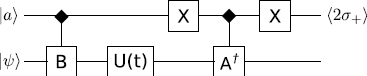
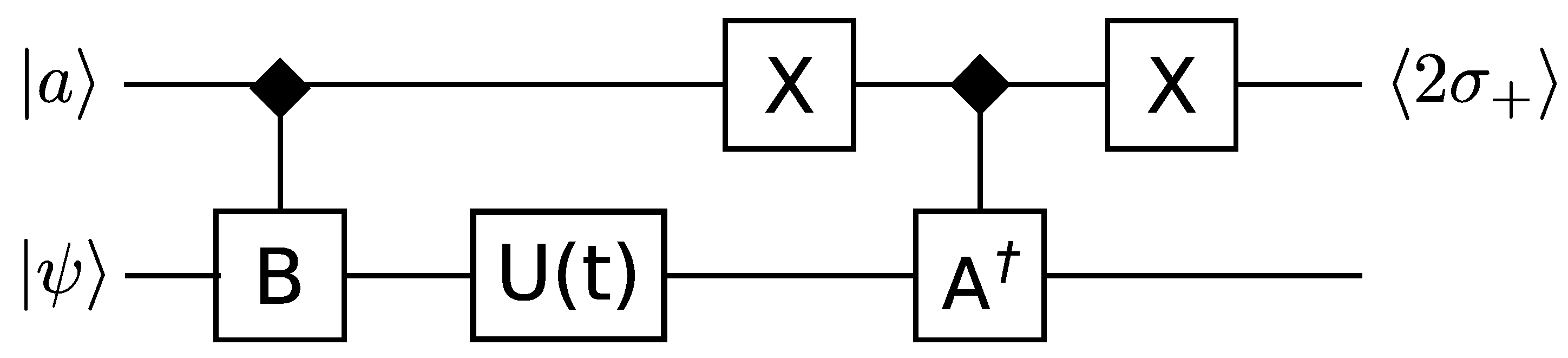
39] provide detailed methods for extracting correlation functions, expectation values of Hermitian operators, and the spectrum of a Hermitian operator. A similar method is employed for all of these, we describe it for correlation functions. A circuit diagram is shown in Figure 1.
This circuit can compute correlation functions of the form
C A B ( t ) = U ^ ( t ) A ^ U ^ ( t ) B ^
where U ^ ( t ) is the time evolution of the system, and A ^ and B ^ are expressible as a sum of unitary operators. The single qubit ancilla | a , initially in the state ( | 0 + | 1 ) / 2 , is used to control the conditional application of B ^ and A ^ , between which the time evolution U ^ ( t ) is performed. Measuring | a then provides an estimate of the correlation function to one bit of accuracy. Repeating the computation will build up a more accurate estimate by combining all the outcomes. By replacing U ^ ( t ) with the space translation operator, spatial correlations instead of time correlations can be obtained.

3.4. Quantum Chaos

The attractions of quantum simulation caught the imagination of researchers in quantum chaos relatively early in the development of quantum computing. Even systems with only a few degrees of freedom and relatively simple Hamiltonians can exhibit chaotic behaviour [44]. However, classical simulation methods are of limited use for studying quantum chaos, due to the exponentially growing Hilbert space. One of the first quantum chaotic systems for which an efficient quantum simulation scheme was provided is the quantum baker’s transformation. Schack [45] demonstrates that it is possible to approximate this map as a sequence of simple quantum gates using discrete Fourier transforms. Brun and Schack [46] then showed that the quantum baker’s map is equivalent to a shift map and numerially simulated how it would behave on a three qubit NMR quantum computer.
While the time evolution methods for chaotic dynamics are straightforward, the important issue is how to extract useful information from the simulation. Using the kicked Harper model, Lévi and Georgeot [47] extended Schack’s Fourier transform method to obtain a range of characteristics of the behaviour in different regimes, with a polynomial speed up. Georgeot [48] discusses further methods to extract information but notes that most give only a polynomial increase in efficiency over classical algorithms. Since classical simulations of quantum chaos are generally exponentially costly, it is disappointing not to gain exponentially in efficiency in general with a quantum simulation. However, there are some useful exceptions: methods for deciding whether a system is chaotic or regular using only one bit of information have been developed by Poulin et al. [49], and also for measuring the fidelity decay in an efficient manner [50]. A few other parameters, such as diffusion constants, may also turn out to be extractable with exponential improvement over classical simulation. A review of quantum simulations applied to quantum chaos is provided by Georgeot [51].

4. Initialization

As we saw in the previous section, a crucial step in extracting useful results from a quantum simulation is starting from the right initial state. These will often be complex or unknown states, such as ground states and Gibbs thermal states. Preparing the initial state is thus as important as the time evolution, and significant research has gone into providing efficient methods. An arbitrary initial state takes exponentially many parameters to specify, see Equation (1), and hence exponential time to prepare using its description. We can thus only use states which have more efficient preparation procedures. Although preparing an unknown state sounds like it should be even harder than preparing a specific arbitrary state, when a simple property defining it is specified, there can be efficient methods to do this.

4.1. Direct State Construction

Where an explicit description is given for the initial state we require, it can be prepared using any method for preparing states for a quantum register. Soklakov and Schack [52,53] provide a method using Grover’s search algorithm, that is efficient provided the description of the state is suitably efficient. Plesch and Brukner [54] optimise general state preparation techniques to reduce the prefactor in the required number of CNOT gates to close to the optimal value of one. Direct state preparation is thus feasible for any efficiently and completely specified pure initial state. Poulin and Wocjan [55] analyse the efficiency of finding ground states with a quantum computer. This is known to be a QMA-complete problem for k-local Hamiltonians (which have the form of Equation (3) where the H j involve k of the variables, for k 2 ). They provide a method based on Grover’s search, with some sophisticated error reduction techniques, that gives a quadratic speed up over the best classical methods for finding eigenvalues of matrices. Their method is really a proof of the complexity of the problem in general rather than a practical method for particular cases of interest, which may not be as hard as the general case they treat.

4.2. Adiabatic Evolution

Adiabatic quantum computing encodes the problem into the ground state of a quantum Hamiltonian. The computation takes place by evolving the Hamiltonian from one with an easy to prepare ground state H ^ 0 to the one with the desired solution H ^ 1 as the ground state,
H ^ ad = ( 1 - s ( t ) ) H ^ 0 + s ( t ) H ^ 1
where the monotonically increasing function s ( t ) controls the rate of change, s ( 0 ) = 0 . This has to be done slowly enough, to keep the system in the ground state throughout. Provided the gap between the ground state and first excited state does not become exponentially small, “slowly enough” will require only polynomial time. Extensive discussion of quantum adiabatic state preparation from an algorithmic perspective, including other useful states that can be produced by this method, is given by Aharonov and Ta Shma [9].
The application to preparing ground states for quantum simulation was first suggested by Ortiz et al. [56]. The potential issue is that finding ground states is in general a QMA-complete problem, which implies it may not be possible to do this efficiently for all cases of interest, that the gap will become exponentially small at some point in the evolution. In particular, we know the gap will become exponentially small if the evolution passes through a quantum phase transition. Since the study of quantum phase transitions is one aspect of quantum many-body systems of interest for quantum simulation, this is not an academic problem, rather, it is likely to occur in practice. Being of crucial importance for adiabatic quantum computation, the question of how the time evolution scales near a phase transition has been extensively studied. Recent work by Dziarmaga and Rams [57] on inhomogeneous quantum phase transitions explains how in many cases of practical interest, disruption to the adiabatic evolution across the phase transition can be avoided. An inhomogeneous phase transition is where the order parameter varies across the system. Experimentally, this is very likely to happen to some extent, due to the difficulty of controlling the driving mechanism perfectly, the strength of a magnetic field for example. Consequently, the phase change will also happen at slightly different times for different parts of the system, and there will be boundaries between the different regions. Instead of being a global change, the phase transition sweeps through the system, and the speed with which the boundary between the phases moves can be estimated. Provided this is slower than the timescale on which local transitions take place, this allows the region in the new phase to influence the transition of the nearby regions. The end result is that it is possible to traverse the phase transition in polynomial time without ending up in an excited state, for a finite-sized system.
Moreover, we don’t generally need to prepare a pure ground state for quantum simulation of such systems. The quantity we usually wish to estimate for a system with an unknown ground state is the energy gap between the ground and first excited states. As described in Section 3.1, this can be done by using phase estimation applied to a coherent superposition of the ground state and first excited state. So traversing the adiabatic evolution only approximately, to allow a small probability of exciting the system is in fact a useful state preparation method. And if we want to obtain the lowest eigenvalues and study the corresponding eigenvectors of a Hamiltonian, again we only need a state with a significant proportion of the ground state as one component, see Section 3.2.
Oh [58] describes a refinement of the Abrams-Lloyd method for finding eigenvalues and eigenvectors described in Section 3.2, in which the state preparation using the adiabatic method is run in parallel with the phase estimation algorithm for estimating the ground state energy. This allows the ground state energy to be extracted as a function of the coupling strength that is increased as the adiabatic evolution proceeds. Oh adds an extra constant energy term to the Hamiltonian, to tune the running time, and uses the Hellman-Feynman theorem to obtain the expectation value of the ground state observable. Boixo et al. [59] prove that this and related methods using continuous measurement, as provided by the phase estimation algorithm run in parallel, improve the adiabatic state preparation. The running time is inversely proportional to the spectral gap, so will only be efficient when the gap remains sufficiently large throughout the evolution.

4.3. Preparing Thermal Equilibrium States

Temperature dependent properties of matter are of key importance. To study these, efficiently preparing thermal states for quantum simulation is crucial. The most obvious method to use is to actually equilibriate the quantum state to the required temperature, using a heat bath. Terhal and DiVincenzo [60] describe how this can be done with only a relatively small bath system, by periodically reinitializing the bath to the required temperature. The core of this algorithm begins by initializing the system in the “all zero” state, | 00 00 00 00 | and the bath in an equilibrium state of the required temperature. The system and bath are then evolved for time t after which the bath is discarded and re-prepared in its equilibrium state. This last step is repeated a number of times, creating to a good approximation the desired thermal initial state for subsequent simulation. Terhal and DiVincenzo don’t give explicit bounds on the running time of their method, though they do discuss reasons why they don’t expect it to be efficient in the general case. Recent results from Poulin and Wocjan [61] prove the upper bound on the running time for thermalisation is D a , where a 1 / 2 is related to the Helmholtz free energy of the system, and D is the Hilbert space dimension. This thus confirms that Terhal and DiVincenzo’s method may not be efficient in general. Poulin and Wocjan also provide a method for approximating the partition function of a system with a running time proportional to the thermalisation time. The partition function is useful because all other thermodynamic quantities of interest can be derived from it. So in cases where their method can be performed efficiently, it may be prefered over the newly developed quantum Metropolis algorithm described next.
The quantum Metropolis algorithm of Temme et al. [62] is a method for efficiently sampling from any Gibbs distribution. It is the quantum analogue of the classical Metropolis method. The process starts from a random energy eigenstate | Ψ i of energy E i . This can be prepared efficiently by evolving from any initial state with the Hamiltonian H ^ , then using phase estimation to measure the energy and thereby project into an eigenstate. The next step is to generate a new “nearby” energy eigenstate | Ψ j of energy E j . This can be achieved via a local random unitary transformation such that | Ψ i j c i j | Ψ j with E j E i . Phase estimation is then used again to project into the state | Ψ j and gives us E j . We now need to accept the new configuration with probability p i j = min [ 1 , exp ( - β ( E i - E j ) ) ] , where β is inverse temperature. Accepting is no problem, the state of the quantum registers are in the new energey eigenstate | Ψ j as required. The key development in this method is how to reject, which requires returning to the previous state | Ψ i . By making a very limited measurement that determines only one bit of information (accept/reject), the coherent part of the phase estimation step can be reversed with high probability; repeated application of the reversal steps can increase the probability as close to unity as required. Intermediate measurements in the process indicate when the reversal has succeeded, and the iteration can be terminated. The process is then repeated to obtain the next random energy state in the sequence. This efficiently samples from the thermal distribution for preparing the initial state, and can be used for any type of quantum system, including fermions and bosons. Temme et al. also prove that their algorithm correctly samples from degenerate subspaces efficiently.

5. Hamiltonian Evolution

The Lloyd method of evolving the quantum state in time according to a given Hamiltonian, described in Section 2.1, is a simple form of numerical integration. There are a variety of other methods for time evolution of the dynamics in classical simulation, some of which have been adapted for quantum simulation. Like their classical counterparts, they provide significant advantages for particular types of problem. We describe two of these methods that are especially promising for quantum simulation: a quantum version of the pseudo-spectral method using quantum Fourier transforms, and quantum lattice gas automata. Quantum chemistry has also developed a set of specialised simulation methods for which we describe some promising quantum counterparts in Section 5.3. We would also like to be able to simulate systems subject to noise or disturbance from an environment, open quantum systems. Some methods for efficiently treating non-unitary evolution are described in Section 5.4.

5.1. Quantum Pseudo-Spectral Method

Fast Fourier transforms are employed extensively in classical computational methods, despite incurring a significant computational cost. Their use can simplify the calculation in a wide diversity of applications. When employed for dynamical evolution, the pseudo-spectral method converts between real space and Fourier space (position and momentum) representations. This allows terms to be evaluated in the most convenient representation, providing improvements in both the speed and accuracy of the simulation.
The same motivations and advantages apply to quantum simulation. A quantum Fourier transform can be implemented efficiently on a quantum computer for any quantum state [63,64]. Particles moving in external potentials often have Hamiltonians with terms that are diagonal in the position basis plus terms that are diagonal in the momentum basis. Evaluating these terms in their diagonal bases provides a major simplification to the computation. Wiesner [65] and Zalka [66,67] gave the first detailed descriptions of this approach for particles moving in one spatial dimension, and showed that it can easily be generalized to a many particle Schrödinger equation in three dimensions. To illustrate this, consider the one-dimensional Schrödinger equation (with = 1 ),
i t Ψ ( x , t ) = - 1 2 m 2 + V ( x ) Ψ ( x , t )
for a particle in a potential V ( x ) . As would be done for a classical simulation this is first discretized so the position is approximated on a line of N positions (with periodic boundary conditions) and spacing Δ x . We can then write the wavefunction as
| Ψ ( n , t ) = n a n ( t ) | n
where { | n } , 0 n < N are position basis states, and a n ( t ) is the amplitude to be at position n at time t. For small time steps Δ t , the Green’s function to evolve from x 1 to x 2 in time Δ t becomes
G ( x 1 , x 2 , Δ t ) = κ exp i m 2 ( x 1 - x 2 ) 2 Δ t + i V ( x 1 ) Δ t
where κ is determined by the normalization. The transformation in terms of basis states is the inverse of this,
G ( n , n , Δ t ) | n = 1 N s n exp - i m 2 ( n - n ) 2 Δ x 2 Δ t - i V ( n Δ x ) Δ t | n
Expanding the square, this becomes
G ( n , n , Δ t ) | n = 1 N exp - i m 2 n 2 Δ x 2 Δ t - i V ( n Δ x ) Δ t × n exp - i m n n Δ x 2 Δ t exp - i m 2 n 2 Δ x 2 Δ t | n
The form of Equation (15) is now two diagonal matrices with a Fourier transform between them, showing how the pseudo-spectral method arises naturally from standard solution methods. Benenti and Strini [68] provide a pedagogical description of this method applied to a single particle, with quantitative analysis of the number of elementary operations required for small simulations. They estimate that, for present day capabilities of six to ten qubits, the number of operations required for a useful simulation is in the tens of thousands, which is many more than can currently be performed coherently. Nonetheless, the efficiency savings over the Lloyd method will still make this the preferred option whenever the terms in the Hamiltonian are diagonal in convenient bases related by a Fourier transform.

5.2. Lattice Gas Automata

Lattice gas automata and lattice-Boltzmann methods are widely used in classical simulation because they evolve using only local interactions, so can be adapted for efficient parallel processing. Despite sounding like abstract models of physical systems, these methods are best understood as sophisticated techniques to solve differential equations: the “gas” particles have nothing directly to do with the particles in the system they are simulating. Instead, the lattice gas dynamics are shown to correspond to the differential equation being studied in the continuum limit of the lattice. Different equations are obtained from different local lattice dynamics and lattice types. Typically, a face-centred cubic or body-centred cubic lattice is required, to ensure mixing of the particle momentum in different directions [69]. Succi and Benzi [70] developed a lattice Boltzmann method for classical simulation of quantum systems, and Meyer [71] applied lattice gas automata to many-particle Dirac systems. Boghosian and Taylor [72] built on this work to develop a fully quantum version of lattice gas automata, and showed that this can be efficiently implemented on a qubit-based quantum computer, for simulations of many interacting quantum particles in external potentials. This method can also be applied to the many-body Dirac equation (relativistic fermions) and gauge field theories, by suitably modifying the lattice gas dynamics, both are briefly discussed by Boghosian and Taylor.
To illustrate the concept, we describe a simple quantum lattice gas in one dimension. This can be encoded into two qubits per lattice site, one for the plus direction and the other for the minus direction. The states of the qubits represent | 1 for a particle present, and | 0 for no particle, with any superposition between these allowed. Each time step consists of two operations, a “collision” operator that interacts the qubits at each lattice site, and a “propagation” operator that swaps the qubit states between neighboring lattice sites, according to the direction they represent. This is like a coined quantum walk dynamics, which is in fact a special case of lattice gas automata, and was shown to correspond to the Dirac equation in the continuum limit by Meyer [71]. Following Boghosian and Taylor [73], we take the time step operator S . C combining both collision C and propagation S to be
S . C q 1 ( x + 1 , t + 1 ) q 2 ( x - 1 , t + 1 ) = 1 2 1 - i - 1 - i - 1 - i 1 + i q 1 ( x , t ) q 2 ( x , t )
where q 1 and q 2 are the states of the two qubits. Taking the continuum limit where the lattice spacing scales as ϵ while the time scales as ϵ 2 gives
t q 1 ( x , t ) = i 2 2 x 2 q 2 ( x , t )
and a similar equation interchanging q 1 and q 2 . Hence for the sum,
t { q 1 ( x , t ) + q 2 ( x , t ) } = i 2 2 x 2 { q 1 ( x , t ) + q 2 ( x , t ) }
The total amplitude ψ ( x , t ) = q 1 ( x , t ) + q 2 ( x , t ) thus satisfies a Schrödinger equation. It is a straightforward generalisation to extend to higher dimensions and more particles, and to add interactions between particles and external potentials, as explained in detail by Boghosian and Taylor [73]. Based on the utility of lattice gas automata methods for classical simulation, we can expect these corresponding quantum versions to prove highly practical and useful when sufficiently large quantum computers become available.

5.3. Quantum Chemistry

Study of the dynamics and properties of molecular reactions is of basic interest in chemistry and related areas. Quantum effects are important at the level of molecular reactions, but exact calculations based on a full Schrödinger equation for all the electrons involved are beyond the capabilities of classical computation, except for the smallest molecules. A hierarchy of approximation methods have been developed, but more accurate calculations would be very useful. Aspuru-Guzik et al. [74] study the application of quantum simulation to calculation of the energies of small molecules, demonstrating that a quantum computer can obtain the energies to a degree of precision greater than that required by chemists for understanding reaction dynamics, and better than standard classical methods. To do this, they adapt the method of Abrams and Lloyd [38] for finding the eigenvalues of a Hamiltonian described in Section 3.2. The mapping of the description of the molecule to qubits is discussed in detail, to obtain an efficient representation. In a direct mapping, the qubits are used to store the occupation numbers for the atomic orbitals: the Fock space of the molecule is mapped directly to the Hilbert space of the qubits. This can be compacted by restricting to the subspace of occupied orbitals, i.e., fixed particle number, and a further reduction in the number of qubits required is obtained by fixing the spin states of the electrons as well. By doing classical simulations of the quantum simulation for H2O and LiH, they show in detail that these methods are feasible. For the simulations, they use the Hartree-Fock approximation for the initial ground state. In some situations, however, this state has a vanishing overlap with the actual ground state. This means it may not be suitable in the dissociation limit or in the limit of large systems. A more accurate approximation of the required ground state can be prepared using adiabatic evolution, see Section 4.2. Aspuru-Guzik et al. confirm numerically that this works efficiently for molecular hydrogen. Data from experiments or classical simulations can be used to provide a good estimate of the gap during the adiabatic evolution, and hence optimise the rate of transformation between the initial and final Hamiltonians.
The Hartree-Fock wavefunctions used by Aspuru-Guzik et al. are not suitable for excited states. Wang et al. [75] propose using an initial state that is based on a multi-configurational self consistent field (MCSCF). These initial states are also suitable for strong interactions, since they avoid convergence to unphysical states when the energy gap is small. In general, using MCSCF wavefunctions allows an evolution that is faster and safer than using Hartree-Fock wavefunctions, so represents a significant improvement.
To calculate the properties of chemical reactions classically, the Born-Oppenheimer approximation is used for the electron dynamics. The same can be done for quantum simulations; however, Kassal et al. [76] observe that, for all systems of more than four atoms, performing the exact computation on a quantum computer should be more efficient. They provide a detailed method for exact simulation of atomic and molecular electronic wavefunctions, based on discretizing the position in space, and evolving the wavefunction using the QFT-based time evolution technique presented by Wiesner [65] and Zalka [66] described in Section 5.1. Kassal et al. discuss three approaches to simulating the interaction potentials and provide the initialisation procedures needed for each, along with techniques for determining reaction probabilities, rate constants and state-to-state transition probabilities. These promising results suggest that quantum chemistry will feature prominently in future applications of quantum simulation.

5.4. Open Quantum Systems

Most real physical systems are subject to noise from their environment, so it is important to be able to include this in quantum simulations. For many types of environmental decoherence, this can be done as a straightforward extension to Lloyd’s basic simulation method [8] (described in Section 2.1). Lloyd discusses how to incorporate the most common types of environmental decoherence into the simulation. For uncorrelated noise, the appropriate superoperators can be used in place of the unitary operators in the time evolution, because these will also be local. Even for the worst case of correlated noise, the environment can be modeled by doubling the number of qubits and employing local Hamiltonians for the evolution of the environment and its coupling, as well as for the system. Techniques for the simulation of open quantum systems for a single qubit have been further refined and developed by Bacon et al. [77], who provide a universal set of processes to simulate general Markovian dynamics on a single qubit. However, it is not known whether these results can be extended to include all Markovian dynamics in systems of more than two qubits, since it is no longer possible to write the dynamics in the same form as for the one and two qubit cases.
Better still, from the point of view of efficiency, is if the effects of noise can be included simply by using the inevitable decoherence on the quantum computer itself. This will work provided the type of decoherence is sufficiently similar in both statistics and strength. Even where the aim is to simulate perfect unitary dynamics, small levels of imperfection due to noisy gates in the simulation may still be tolerable, though the unfavorable scaling of precision with system size discussed in Section 2.2 will limit this to short simulations. Nonetheless, in contrast to the error correction necessary for digital quantum computations where precise numerical answers are required, a somewhat imperfect quantum simulation may be adequate to provide us with a near perfect simulation of an open quantum system.

6. Fermions and Bosons

Simulation of many-body systems of interacting fermions are among the most difficult to handle with classical methods, because the change of sign when two identical fermions are exchanged prevents the convergence of classical statistical methods, such as Monte Carlo sampling. This is known as the “sign problem”, and has limited effective simulation of fermionic many-body systems to small sizes that can be treated without these approximations. Very recent work from Verstraete and Cirac [78] has opened up variational methods for fermionic systems, including relativistic field theories [79]. Nonetheless, the computational cost of accurate classical simulations is still high, and we have from Ortiz et al. [56] a general proof that conducting a simulation of a fermionic system on a quantum computer can be done efficiently and does not suffer from the sign problem. They also confirm that errors within the quantum computation don’t open a back door to the sign problem. This clears the way for developing detailed algorithms for specific models of fermionic systems of particular interest. Some of the most important open questions a quantum computer of modest size could solve are models involving strongly interacting fermions, such as for high temperature superconductors.

6.1. Hubbard Model

One of the important fermionic models that has received detailed analysis is the Hubbard model, one of the most basic microscopic descriptions of the behaviour of electrons in solids. Analytic solutions are challenging, especially beyond one dimension, and while ferromagnetism is obtained for the right parameter ranges, it is not known whether the basic Hubbard model produces superconductivity. The difficulties of classical simulations thus provide strong motivation for applying quantum simulation to the Hubbard model. The Hubbard Hamiltonian H ^ γ V is
H ^ γ V = - γ j , k , σ C ^ j , σ C ^ k , σ + V j n ^ j , n ^ j ,
where C ^ j , σ C ^ k , σ are the fermionic creation and annihilation operators, σ is the spin (up or down), n ^ j , n ^ j , are the number operators for up spin and down spin states at each site j, γ is the strength of the hopping between sites, and V is the on site potential. Abrams and Lloyd [80] describe two different encodings of the system into the quantum simulator. An encoding using the second quantization is more natural since the first quantization encoding requires the antisymmetrization of the wavefunction “by hand”. However, when the number of particles being simulated is a lot lower than the available number of qubits, the first quantization is more efficient. In second quantization, there are four possible states each site can be in: empty, one spin up, one spin down, and a pair of opposite spin. Two qubits per site are thus required to encode which of the four states each site is in. It is then a simple extension of the Lloyd method to evolve the state of the system according to the Hubbard Hamiltonian. Somma et al. [39] describe how to use this method to find the energy spectrum of the Hubbard Hamiltonian for a fermionic lattice system. They perform a classical computer simulation of a quantum computer doing a quantum simulation, to demonstrate the feasibility of the quantum simulation. The Hubbard model is the natural Hamiltonian in optical lattice schemes, so there has been considerable development towards special purpose simulators based on atoms in optical lattices, these are discussed in Section 9.2.

6.2. The BCS Hamiltonian

Pairing Hamiltonians are an important class of models for many-body systems in which pairwise interactions are typically described using fermionic (or bosonic) creation and annihilation operators { c m , c m } . Nucleons in larger atomic nuclei can be described by pairing Hamiltonians, and Bardeen, Copper and Schrieffer (BCS) [81] formulated a model of superconductivity as a a pairing Hamiltonian in the 1950s. The BCS model of superconductivity is still not fully understood, so quantum simulations could be useful to improve our knowledge of superconducting systems, especially for realistic materials with imperfections and boundary effects. While the BCS ansatz is exact in the thermodynamic limit, it is not known how well it applies to small systems [82].
The BCS Hamiltonian for a fully general system can be written
H B C S = m = 1 N ϵ m 2 ( c m c m + c - m c - m ) + m , l = 1 N V m l c m c - m c - l c l
where the parameters ϵ m and V m l specify the self energy of the mth mode and the interaction energy of the mth and lth modes respectively, while N is the total number of occupied modes (pairs of fermions with opposite spin). Wu et al. [37] developed a detailed method for quantum simulation of Equation (20). The two terms in the BCS Hamiltonian do not commute, therefore the simulation method requires the use of Trotterization (see Section 2.1) so the two parts can be individually applied alternately. This means that any simulation on a universal quantum computer will require many operations to step through the time evolution, which will stretch the experimentally available coherence times. Savings in the number of operations are thus important, and recent work by Brown et al. [83] adapting the method to a qubus architecture reduces the number of operations required in the general case from O ( N 5 ) for NMR to O ( N 2 ) for the qubus. Pairing Hamiltonians are used to describe many processes in condensed matter physics and therefore a technique for simulating the BCS Hamiltonian should be adaptable to numerous other purposes.

6.3. Initial State Preparation

For simulation on qubit quantum computers (as opposed to special purpose quantum simulators), we first need an efficient mapping between the particles being simulated and the spin-1/2 algebra of the qubit systems. Somma et al. [84] discuss in detail how to map physical particles onto spin-1/2 systems. For fermions there is a one-to-one mapping between the fermionic and spin-1/2 algebras. Particularly in the second quantization this allows a simple mapping that can be generalised to all anyonic systems which obey the Pauli exclusion principle, or generalised versions of it. For bosonic systems there is no direct mapping between the bosonic algebra and spin 1/2 algebra. Therefore Somma et al. propose using a direct mapping between the state of the two systems, provided there is a limit on the number of bosons per state. This mapping is less efficient but allows simulations to be conducted on the bosonic systems.
Systems of indistinguishable particles require special state preparation to ensure the resulting states have the correct symmetry. Ortiz et al. [56] developed a method for fermions that was then adapted for bosons by Somma et al. [84]. In general, a quantum system of N e fermions with an anti-symmetrized wavefunction | Ψ e can be written as a sum of Slater determinants | Φ α
| Ψ e = α = 1 n a α | Φ α
where n is an integer and α = 1 n | a α | 2 = 1 . The individual Slater determinants can be prepared efficiently using unitary operations. Provided the desired state doesn’t require an exponential sum of Slater determinants, with the help of n ancilla qubits it is possible to prepare the state
α = 1 n a α | α | Φ α
where | α is a state of the ancilla with the α’th qubit in state | 1 and the rest in state | 0 . A further register of n ancillas is then used to convert the state so that there is a component with the original ancillas in the all zero state,
α = 1 n a α | 0 a | Φ α
associated with the required state of the fermions. A measurement in the z-basis selects this outcome (all zeros) with a probability of 1 / n . This means the preparation should be possible using an average of n trials.
A general bosonic system can be written as a linear combination of product states. These product states can be mapped onto spin states and then easily prepared by flipping the relevant spins. Once the bosonic system has been written as a linear combination of these states, a very similar preparation procedure to the one for fermionic systems can be used [84].
While the above method using Slater determinants is practical when working in second quantization, this isn’t always convenient for atomic and molecular systems. Ward et al. [85] present a system for efficiently converting states prepared using Slater determinants in second quantization to a first quantization representation on a real space lattice. This can be used for both pure and mixed states.

6.4. Lattice Gauge Theories

Lattice gauge theories are important in many areas of physics, and one of the most important examples from a computational perspective is quantum chromodynamics (QCD). Classical QCD simulations are extremely computationally intensive, but very important for predicting the properties of fundamental particles. Providing more efficient quantum simulations would be very useful to advance the field. The quantum lattice gas method developed by Boghosian and Taylor [73] (discussed in Section 5.2) is suitable for simulating lattice gauge theories, using similar methods to the lattice QCD simulations currently performed classically, but with the benefit of a quantum speed up. Byrnes and Yamamoto [86] provide a more general method. They map the desired Hamiltonian to one involving only Pauli operations and one and two qubit interactions. This is then suitable for any qubit-based universal quantum simulator. They focus on the U(1), SU(2) and SU(3) models, but their methods easily generalise to higher order SU(N) theories. To conduct the simulation efficiently it is necessary to use a truncated version of the model, to keep the number of qubits finite. They demonstrate that the number of operations required for the time evolution and for the preparation of the necessary initial states are both efficient. To get results inaccessible to classical computers, of the order of 10 5 qubits will be required. Despite this, the algorithm has advantages over classical techniques because the calculations are exact up to a cut off, and with simple adaptions it can be extended to to simulate fermionic systems.
Methods suitable for special purpose quantum simulators have been presented by Schützhold and Mostame [87] and Tewari et al. [88]. Schützhold and Mostame describe how to simulate the O(3) nonlinear σ-model, which is of interest to the condensed matter physics community as it applies to spin systems. It also reproduces many of the key properties of QCD, although it is only a toy model in this context. To conduct their simulation, Schützhold and Mostame propose using hollow spheres to trap electrons, described in more detail in Section 10.1. Tewari et al. [88] focus specifically on compact U(1) lattice gauge theories that are appropriate for dipolar bosons in optical lattices. The basic Hamiltonian in optical lattices is the Hubbard Hamiltonian, Equation (19), but different choices of atom can enhance the Hamiltonian with different nearest neighbour interactions. The specific example chosen by Tewari et al. is chromium, which has a magnetic dipolar interaction that can provide the extra term in the Hamiltonian. The ratio of the two types of couplings (Hubbard and dipolar) can be varied over a wide range by tuning the Hubbard interaction strength using Feshbach resonances. Further types of relativistic quantum field theories that can be simulated by atoms in optical lattices are presented by Cirac et al. [89].
This concludes the theory part of our review, and provides a natural point to move over to consideration of the different physical architectures most suited to quantum simulation.

7. Overview

As we have seen, while algorithms for quantum simulation are interesting in their own right, the real drive is towards actual implementations of a useful size to apply to problems we cannot solve with classical computers. The theoretical studies show that quantum simulation can be done with a wide variety of methods and systems, giving plenty of choices for experimentalists to work with. Questions remain around the viability of longer simulations, where errors may threaten the accuracy of the results, and long sequences of operations run beyond the available coherence times. As with quantum computing in general, the main challenge for scaling up is controlling the decoherence and correcting the errors that accumulate from imperfect control operations. Detailed treatment of these issues is beyond the scope of this review and well-covered elsewhere (see, for example, Devitt et al. [90]). The extra concern for quantum simulation lies in the unfavorable scaling of errors with system size, as discussed in Section 2.2.
In Section 2 we described how to obtain universal quantum simulation from particular sets of resources, mainly a fixed interaction with local unitary controls. Building a universal quantum simulator will allow us to efficiently simulate any quantum system that has a local or efficiently describable Hamiltonian. On the other hand, the generality of universal simulation may not be necessary if the problem we are trying to solve has a specific Hamiltonian with properties or symmetries we can exploit to simplify the simulation. If the Hamiltonian we want to simulate can be matched with a compatible interaction Hamiltonian in the quantum simulator, then there are are likely to be further efficiencies available through simpler control sequences for converting one into the other. From the implementation perspective, a special purpose simulator may be easier to build and operate, a big attraction in these early stages of development. Most architectures for quantum computing are also suitable for universal quantum simulation. However, the range of experimental possibilities is broader if we are willing to specialise to the specific Hamiltonians in the quantum simulator. This allows more to be achieved with the same hardware, and is thus the most promising approach for the first useful quantum simulations.
Buluta and Nori [91] give a brief overview of quantum simulation that focuses on the various possible architectures and what sort of algorithms these could be used for. There is broad overlap of relevant experimental techniques with those for developing quantum computers in general, and many issues and considerations are common to all applications of quantum computers. In this paper, we concentrate on implementations that correspond to the theoretical aspects we have covered. Many experimental implementations of quantum simulation to date have been in NMR quantum computers. This is not a scalable architecture, but as a well-developed technology it provides an invaluable test bed for small quantum computations. Optical schemes based on entangled photons from down-conversion have also been used to implement a variety of small quantum simulations, but since photons don’t normally interact with each other, they don’t provide a natural route to special purpose quantum simulators. We describe the lessons learned from these quantum simulations in Section 8. We then turn to simulators built by trapping arrays of ions, atoms, and electrons in Section 9 and Section 10. Most of these have applications both as universal quantum simulators and for specific Hamiltonians, with promising experiments and rapid progress being made with a number of specific configurations.

8. Proof-of-Principle Experiments

Some of the most advanced experimental tests of quantum computation have been performed using technology that does not scale up beyond ten or so qubits. Nonetheless, the information gained from these experiments is invaluable for developing more scalable architectures. Many of the control techniques are directly transferable in the form of carefully crafted pulse sequences with enhanced resilience to errors and imperfections. Observing the actual effects of decoherence on the fidelities is useful to increase our understanding of the requirements for scaling up to longer sequences of operations.

8.1. NMR Experiments

Nuclear Magnetic Resonance is a highly developed technology that provides an adaptable toy system for quantum computing (see Jones [92] for a comprehensive review). A suitable molecule with atoms having various nuclear spins is prepared, often requiring chemical synthesis to substitute different isotopes with the required spins. A solution of this molecule then provides an ensemble which can be collectively controlled by applied magnetic fields and radio frequency (rf) pulses. The nuclear spins of the different atomic species will in general have different resonant frequencies, allowing them to be addressed separately. Read out is provided by exploiting spin echo effects. Liquid state NMR isn’t considered to be scalable due to the difficulty of addressing individual qubits in larger molecules. Nonetheless, the relative ease with which quantum algorithms can be implemented for small systems has meant that many proof-of-principle experiments have been carried out using NMR. These are often of only the smallest non-trivial size, using as few as one or two qubits, but are still useful for developing and testing the control sequences. The real advantage lies in the flexibility of applying gates through radio frequency (RF) pulses. This allows NMR to outperform other test-bed systems such as optics, where each gate requires its own carefully aligned components on the bench. Since most quantum algorithms have been tested in NMR by now, we select for discussion a few that bring out important points about the experimental feasibility of quantum simulation in general.
Numerous groups have performed NMR quantum simulations of spin chains. The Heisenberg interaction is already present in NMR in the form of the Z Z interaction (X, Y, Z are used to denote the Pauli spin operators). This allows more complex Heisenberg interactions to be simulated by using local unitary operations to rotate the spin between the X, Y and Z orientations. These simulations are thus a simple example of using one fixed Hamiltonian— Z Z in this case—to simulate another, as described theoretically in Section 2. This allows the investigation of interesting properties of these spin chains such as phase transitions [93,94], the propagation of excitons [95] and the evolution under particular interactions [96]. Peng et al. [93] and Khitrin et al. [95] found that the decoherence time of the system is often too short to get meaningful results, even for these small simulations. The limited decoherence times were turned into an advantage by Alvarez et al. [97], to study the effects on quantum information transfer in spin chains. As expected, they were able to show that decoherence limits the distance over which quantum information can be transferred, as well as limiting the time for which it can be transferred. This is an example of using the noise naturally present in the quantum computer to simulate the effects on the system under study, as described in Section 5.4.
Tseng et al. [98] describe how to simulate a general three-body interaction using only the Z Z interaction present in NMR, and experimentally demonstrated a Z Z Z interaction. This provided proof of principle for extending the repertoire of NMR quantum simulation beyond two-body Hamiltonians, later comprehensively generalised theoretically by Dür et al. [31] (see Section 2.3). Liu et al. [99] demonstrated experimentally that four-body interactions in a four qubit NMR quantum computer can be simulated to within good agreement of their theoretical calculations.
Pairing Hamiltonians (see Section 6.2) are of particular importance for quantum simulation, with the fermionic systems they describe including superconductors and atomic nuclei. The long range interactions put simulation of general pairing systems beyond the reach of classical computers. Studies using NMR have focused on the BCS Hamiltonian, Equation (20), which is a pairing Hamiltonian with interactions composed of Pauli spin operators. However, because it consists of two non-commuting parts, these have to be implemented individually and then recombined using the Trotter-Suzuki formula, as described in Section 2.1. Wu et al. [37] provided a detailed discussion of how to make this efficient for NMR, and their method was implemented experimentally by Brown et al. [13] on three qubits. As well as their insightful comments on the scaling of errors in the simulation, discussed in Section 2.2, they also added artificial noise to their simulations to verify the scaling. This confirmed that simulation of larger systems will be challenging, due to the high number of operations required for the Trotter expansion, and correspondingly large error correction overheads.
Negrevergne et al. [100] simulate a many-body Fermi system that obeys the Fano-Anderson model, a ring system with an impurity at the centre. This can be done with three NMR qubits, once the translational symmetry in the ring has been taken into account and the fermion modes mapped to the qubits. To minimise problems with decoherence caused by running the system for a long time, Negrevergne designed and implemented an approximate refocusing scheme. This provided a scalable algorithm, which can be adapted to other architectures as more powerful quantum simulators are built.
Although bosons are easier to simulate classically than fermions (because they don’t suffer from the “sign problem”) for quantum simulations they are harder, due to the unlimited size of the Hilbert space. The Hilbert space has to be artificially truncated, and this limits the accuracy. Simulations of a bosonic system have been carried out by Somaroo et al. [101], who chose the truncated harmonic oscillator. The limitations due to the truncation are quite significant in a small NMR simulation, and scaling up would be difficult, as a larger system would require small couplings within the NMR simulator that would severely limit the time scale of the experiment. As with other simulations, the decoherence time limits the duration of the experiment, which in this case corresponds to the number of periods of the oscillator which can be simulated.
Du et al. [102] have simulated molecular hydrogen in order to obtain its ground state energy. To do this they use the algorithm presented by Aspuru-Guzik et al. [74], described in Section 5.3. This is an important class of quantum simulations, because it turns out to be more efficient in the quantum case to simulate the dynamics exactly, instead of following the approximations used to do these calculations classically. They thus offer the possibility of significant improvements for quantum chemistry, given a large enough quantum computer. With NMR systems, the simulations are limited to hydrogen, and while the decomposition of the molecular evolution operator scales efficiently, Du et al. [102] are not sure whether the same is true of their adiabatic state preparation method. Nonetheless, this is an important proof of principle for the method and application.

8.2. Photonic Systems

Linear optics, with qubits encoded in the photonic degrees of freedom, are an attractive option for quantum computing due to the relatively straightforward experimental requirements compared to architectures requiring low temperatures and vacuum chambers. The main difficulty is obtaining a suitable nonlinear interaction, without which only regimes that can be simulated efficiently classically can be reached. Current experiments generally use less scalable techniques for generating the nonlinear operation, such as using entangled pairs of photons from down-conversion in nonlinear crystals, or measurements with probabilistic outcomes, so the experiment has to be repeated until it succeeds.
Lanyon et al. [103] used the algorithm presented by Aspuru-Guzik et al. [74] to simulate molecules. The qubits were encoded in the polarisation of single photons, with linear optical elements and a nonlinearity obtained through projective measurements used to provide the necessary control. Ma et al. [104] used the polarisation states of four photons to simulate a spin system of four spin - 1 / 2 particles with arbitrary Heisenberg-type interactions between them. They used measurements to induce the interaction between the spins, and were able to measure ground state energy and quantum correlations for the four spins.
While photonic systems do not have an intrinsic Hamiltonian that is adaptable for special purpose quantum simulation, they are expected to come into their own as universal quantum computers. There are strong proposals for scalable architectures based on photonic systems [105,106] that can also be exploited for quantum simulation.

9. Atom Trap and Ion Trap Architectures

Among the architectures for quantum computing predicted to be the most scalable, qubits based on atoms or ions in trap systems are strongly favoured [107,108]. Locating the atoms or ions in a trap allows each qubit to be distinguished, and in many cases individually controlled. Review of the many designs that are under development is beyond the scope of this article; while any design for a quantum computer is also suitable for quantum simulation, we focus here on arrays of atoms or ions where the intrinsic coupling between them can be exploited for quantum simulation.
Trapped ions form a Coulomb crystal due to their mutual repulsion, which separates them sufficiently to allow individual addressing by lasers. Coupling between them can be achieved via the vibrational modes of the trap, or mediated by the controlling lasers. Atoms in optical lattices formed by counter-propagating laser beams are one of the most promising recent developments. Once the problem of loading a single atom into each trap was overcome by exploiting the Mott transition [109], the road was clear for developing applications to quantum computing and quantum simulation. For comprehensive reviews of experimental trap advances, see Wineland [110] for ion trapping, and Bloch et al. [111] for cold atoms.
Jané et al. [112] consider quantum simulation using both neutral atoms in an optical lattice and ions stored in an array of micro traps. This allows them to compare the experimental resources required for each scheme, as well as assessing the feasibility of using them as a universal quantum simulator. Atoms in optical lattices have the advantage that there is a high degree of parallelism in the manipulation of the qubits. The difficulty of individually addressing each atom, due to the trap spacing being of the same order as the wavelength of the control lasers, can be circumvented in several ways. If the atoms are spaced more widely, so only every fifth or tenth trap is used, for example, then individual laser addressing can be achieved. Applied fields that intersect at the target atom can also be used to shift the energy levels such that only the target atom is affected by the control laser. Jané et al. conclude that both architectures should be suitable for quantum simulation.
An alternative approach is to avoid addressing individual atoms altogether. Kraus et al. [113] explore the potential of simulations using only global single-particle and nearest neighbor interactions. This is a good approximation for atoms in optical lattices, and the three types of subsystem they consider—fermions, bosons, and spins—can be realised by choosing different atoms to trap in the optical lattice and tuning the lattice parameters to different regimes. They make the physically reasonable assumption that the interactions are short range and translationally invariant. They also apply an additional constraint of periodic boundary conditions, to simplify the analysis. Most physical systems have open rather than periodic boundary conditions, so their results may not be immediately applicable to experiments. For a quadratic Hamiltonian acting on fermions or bosons in a cubic lattice, Kraus et al. found that generic nearest neighbor interactions are universal for simulating any translationally invariant interaction when combined with all on-site Hamiltonians (the equivalent of any local unitary) provided the interactions acted along both the axes and diagonals of the cubic lattice (compare lattice gases, Section 5.2). However, for spins in a cubic lattice, there is no set of nearest-neighbor interactions which is universal and not even all next-to-nearest neighbor interactions could be simulated from nearest-neighbor interactions. It is possible that different encodings to those used by Kraus et al. could get around this restriction, but the full capabilities of spin systems on a cubic lattice remains an open problem. Their results demonstrate that schemes which don’t provide individual addressability can still be useful for simulating a large class of Hamiltonians.
Coupled cavity arrays are a more recent development, combining the advantages a cavity confers in controlling an atom with the scalability of micro-fabricated arrays. While there is a trade off between the relative advantages of the various available trapping architectures, with individual addressability and greater control resulting in systems with a poorer scaling in precision, each scheme has its own advantages and the experiments are still in the very early stages.

9.1. Ion Trap Systems

The greater degree of quantum control available for ions in traps, compared with atoms in optical lattices, means that research on using ion traps for simulating quantum systems is further developed. Clark et al. [114] and Buluta and Hasegawa [115] present designs based on planar RF traps that are specifically geared towards quantum simulations. They focus on producing a square lattice of trapped ions, but their results can be generalised to other shapes such as hexagonal lattices (useful for studying systems such as magnetic frustration). Clark et al. carried out experimental tests on single traps that allowed them to verify their numerical models of the scheme are accurate. They identify a possible difficulty when it is scaled to smaller ion-ion distances. As the ion spacing decreases, the secular frequency increases, which may make it difficult to achieve coupling strengths that are large relative to the decoherence rate.
As with the simulations done with NMR computers, some of the earliest work on ion trap simulators has focused on the simulation of spin systems. Deng et al. [116] and Porras and Cirac [117,118] discuss the application of trapped ions to simulate the Bose-Hubbard model, and Ising and Heisenberg interactions. This would allow the observation and analysis of the quantum phase transitions which occur in these systems. They mention three different method for trapping ions that could be used to implement their simulation schemes. Arrays of micro ion traps and linear Paul traps use similar experimental configurations, although Paul traps allow a long range interaction that micro ion trap arrays don’t. Both schemes are particularly suited to simulating an interaction of the form XYZ. Penning traps containing two-dimensional Coulomb crystals could also be used, and this would allow hexagonal lattices to be applied to more complex simulations, such as magnetic frustration. Alternatively [118], the phonons in the trapped ions can be viewed as the system for the simulation. Within the ion trap system phonons can neither be created nor destroyed, so it is possible to simulate systems such as Bose-Einstein condensates, which is more difficult using qubit systems.
Friedenauer et al. [119] have experimentally simulated a quantum phase transition in a spin system using two trapped ions. The system adiabatically traverses from the quantum paramagnetic regime to the quantum (anti)-ferromagnetic regime, with all the parameters controlled using lasers and RF fields. To extract data over the full parameter range the experiment was repeated 10 4 times, to obtain good statistics for the probability distributions. While the simulation method is scalable, involving global application of the control fields, it isn’t clear the data extraction methods are practical for larger simulations. This work is significant for being one of the few detailed proof-of-concept experimental studies done in a system other than NMR, and demonstrates the progress made in developing other architectures. In Gerritsma et al. [120], they simulate the Klein paradox, in which electrons tunnel more easily through higher barriers than low ones, by precisely tuning the parameters in their trapped ion system. Edwards et al. [121] have simulated an Ising system with a transverse field using three trapped ions. They alter the Hamiltonian adiabatically to study a wide range of ground state parameters, thereby mapping out the magnetic phase diagram. This system is scalable up to many tens of ions, which would reach regimes currently inaccessible to classical computation, allowing behavior towards the thermodynamic limit to be studied in detail for general and inhomogeneous spin systems.
Proof-of-principle simulations have also been done with single ions. While less interesting than coupled ions, because the coupled systems are where the Hilbert space scaling really favours quantum simulations, these still test the controls and encoding required. For example, Gerritsma et al. [122] simulated the Dirac equation using a single trapped ion, to model a relativistic quantum particle. The high level of control the ion trap provides allows information about regimes and effects that are difficult to simulate classically such as Zitterbewegung.

9.2. Atoms in Optical Lattices

Atoms trapped in the standing waves created by counter-propagating lasers are one of the most exciting recent developments in quantum computing architectures. Their potential for the quantum simulation of many-body systems was obvious from the beginning, and has been studied by many groups since the initial work of Jané et al. [112]. Trotzky et al. [123] compare optical lattice experimental data with their own classical Monte Carlo simulations, to validate the optical lattice as a reliable model for quantum simulations of ultra-cold strongly interacting Bose gases. They find good agreement for system sizes up to the limit of their simulations of 3 × 10 5 particles.
The most promising way to use atoms in optical lattices for quantum simulation is as a special purpose simulator, taking advantage of the natural interactions between the atoms. This will allow larger systems to be simulated well before this becomes possible with universal quantum computers. The following three examples illustrate the potential for thinking creatively when looking for the best methods to simulate difficult systems or regimes. Johnson et al. [124] discuss the natural occurrence of effective three-body and higher order interactions in two-body collisions between atoms in optical lattices. They use these to explain experimental results showing higher-than-expected decoherence rates. Tuning these many-body interactions could be done using Feshbach resonance control or manipulating the lattice potentials, allowing them to be used for the simulation of effective field theories, see Section 5.2. Ho et al. [125] propose that simulating the repulsive Hubbard model is best done using the attractive Hubbard model, which should be easier to access experimentally. Mapping between different regimes in the same model should be simpler to implement, allowing access to results that are usually difficult experimentally. As with the trapped ion schemes, one of the most common subjects for simulation is many-body quantum phase transitions. Kinoshita et al. [126] use rubidium-87 atoms trapped in a combination of two light traps. By altering the trap strengths, the interactions between the atoms can be controlled, allowing them to behave like a one-dimensional Tonks-Girardeau gas through to a Bose-Einstein condensate. They find very good agreement with theoretical predictions for a 1D Bose gas. This is a good example of a special purpose simulator, since there are no individual controls on the atoms, allowing only regimes dictated by the globally controlled coupling to be realised.

9.3. Atoms in Coupled Cavity Arrays

Optical lattices are not the only way to trap arrays of atoms. Coupled cavity arrays offer control over individual atoms much more conveniently than with optical lattices. In coupled cavities the qubits are represented by either polaritons or hyperfine ground state levels, with the former allowing continuous control, and the latter individual addressability. The cavities themselves are an artificial system grown on a microchip in which the qubits on the chip interact with the field mode of the cavity, and the cavities are coupled by the exchange of photons. A simulation of the Heisenberg model is generally one of the earliest proof-of-principle simulations for a new architecture, and Cho et al. [127] propose a technique to allow these coupled cavity arrays to do this. Their method should apply generally to different physical implementations of micro cavities. Kay et al. [128] and Chen et al. [129] both discuss implementation of the Heisenberg model in specific coupled cavity architectures. They confirm that control over nearest and next-nearest neighbour coupling can be achieved, but without short control pulses only global controls are available. Schemes that give individual addressability need short control pulses to modify the intrinsic interactions. These may necessitate the use of the Trotter approximation, making it more difficult to obtain high precision results in cavity arrays. Ivanov et al. [130] look at exploiting the polaritons in couple cavity arrays to simulate phase transitions, in the same way as Porras and Cirac [118] consider using phonons in ion traps. These proposals show the versatility and potential of coupled cavity arrays for further development.

10. Electrons and Excitons

While atoms and ions in arrays of traps are the most promising scalable architectures for quantum simulation at present, electrons can also be controlled and trapped suitably for quantum simulation. This can be done either by confining free electrons, or exploiting the electrons-hole pairs in quantum dots. Superconducting qubits harness collective states of electrons or quantized flux to form qubits from superconducting circuits with Josephson junctions. We briefly describe applications of these architectures to quantum simulations that exploit their special features.

10.1. Spin Lattices

Spin lattices are arrays of electrons, where the spin of the electron is used as the qubit. Persuading the electrons to line up in the required configuration can be done in various ways. Mostame and Schützhold [131] propose to trap electrons using pairs of gold spheres attached to a silicon substrate under a thin film of helium. The electrons float on the surface of the helium and induce a charge on the spheres, which generates a double well potential and hence traps the electrons. Mostame and Schützhold describe how to use this architecture to simulate an Ising spin chain, from which the generalisation to more complicated models can easily be made. This model for trapping electrons is suggested to be more scalable than atom or ion traps. However, it may be difficult to realise experimentally, due to the precise controls needed, particularly in the thickness of the film of helium. Byrnes et al. [132] propose to confine a 2D electron gas using surface acoustic waves to create an `egg-carton’ potential. The advantage that this system has over optical lattices is that it produces long range interactions. It should therefore be more suitable for simulating Hubbard dynamics, which originate from the long range Coulomb interaction. This scheme will allow observations of quantum phase transitions in systems of strongly correlated electrons as well as the study of the metal-insulator transition.

10.2. Quantum Dots

The trapped electrons or holes in a semiconductor quantum dot can be exploited as qubits, with control provided via gate electrodes or optical fields. Instead of focusing on just the qubit degrees of freedom, the whole quantum dot can be thought of as an artificial atom, which may thus make them suitable to simulate chemical reactions. Quantum dots are now easy to make; the problem is to control their parameters and location so they can be used collectively in a predictable manner. Smirnov et al. [133] discuss using the coupling of quantum dots to model bond formation. They consider one of the simplest possible systems for proof of principle calculations, the interaction H + H 2 H 2 + H , where the molecular bond between a pair of hydrogen atoms switches to a different pair. This can be simulated with a system of three coupled quantum dots, such as has been demonstrated experimentally [134,135]. The high level of control in quantum dot systems will allow the detailed study of chemical reactions in conditions not available in real molecules.

10.3. Superconducting Architectures

Superconducting architectures have been developing steadily although in general they are a few years behind the atom and ion trap systems. As universal quantum computers they are equally suitable in principle for quantum simulation. Charge, phase and flux qubits can be constructed using Josephson junction superconducting circuits, with controls provided by a variety of externally applied fields.
An ingenious proposal from Pritchard et al. [136] describes how to use a systems of Josephson junctions for simulation of molecular collisions. The simulations are restricted to the single excitation subspace of an n - qubit system, which requires only an n × n -dimensional Hamiltonian. In return for this subspace restriction, the individual parameters in the Hamiltonian can be varied independently, providing a high level of generality to the simulation. They use a time-dependent rescaling of time to optimise the actual run time of the simulation to minimise decoherence effects. They test their method in an experiment with three tunable coupled phase qubits simulating a three-channel molecular collision between Na and He. They study the fidelities achieved, and determine the relationship between the fidelity and length of time the simulation is run for. Higher fidelities require longer simulation times, but this is independent of n, showing this aspect of the method is fully scalable.

11. Outlook

Quantum simulation is one of the primary short- to mid-term goals of many research groups focusing on quantum computation. The potential advances that even a modest quantum simulator would unleash are substantial in a broad range of fields, from material science (high temperature superconductors and magnetic materials) to quantum chemistry. Quantum simulations are particular promising for simulating fermionic many-body systems and their phase transitions, where the “sign problem” limits efficient classical numerical approximation techniques. Larger quantum simulators could tackle problems in lattice QCD that currently consume a sizable fraction of scientific computing power, while quantum simulations of quantum chemistry have wide-ranging applications reaching as far as the design of molecules for new drugs. We have seen that the theoretical foundations have been laid quite comprehensively, providing detailed methods for efficient quantum simulators, and calculations that confirm their viability.
One significant issue that remains to be fully addressed is the precision requirements for larger scale quantum simulations. Due to the one-to-one mapping between the Hilbert space of the system and the Hilbert space of the quantum simulator, the resources required for a given precision scale inversely with the precision. Compared with digital (classical and qubit) computations, this is exponentially more costly. When combined with the long control sequences required by Trotterization, this threatens the viability of such simulations of even fairly modest size.
Special purpose quantum simulators designed with similar Hamiltonians to the quantum system being studied are the front runners for actually performing a useful calculation beyond the reach of conventional computers. These come in many forms, matching the variety of common Hamiltonians describing physical systems. Among the most developed and versatile, ion traps and atoms in optical lattices are currently in the lead, although micro-fabrication techniques are allowing more sophisticated solid state trap arrays to catch up fast. Actual experimental systems capable of quantum simulations of a significant size are still in the future, but the designs and proof-of-concept experiments already on the table provide a strong base from which to progress on this exciting challenge.

Acknowledgments

We thank Clare Horsman for careful reading of the manuscript. KLB is supported by a UK EPSRC CASE studentship from Hewlett Packard. VMK is funded by a UK Royal Society University Research Fellowship. WJM acknowledges part support from MEXT in Japan.

References

  1. Raedt, K.D.; Michielsen, K.; Raedt, H.D.; Trieu, B.; Arnold, G.; Richter, M.; Lippert, T.; Watanabe, H.; Ito, N. Massive Parallel Quantum Computer Simulator. Comp. Phys. Comm. 2007, 176, 121–136. [Google Scholar] [CrossRef]
  2. Verstraete, F.; Porras, D.; Cirac, J.I. Density Matrix Renormalization Group and Periodic Boundary Conditions: A Quantum Information Perspective. Phys. Rev. Lett. 2004, 93, 227205. [Google Scholar] [CrossRef] [PubMed]
  3. Feynman, R.P. Simulating Physics wih Computers. Int. J. Theoret. Phys. 1982, 21, 467–488. [Google Scholar] [CrossRef]
  4. Deutsch, D. Quantum-theory, the Church-Turing Principle and the Universal Quantum Computer. Proc. R. Soc. Lond. A 1985, 400, 97–117. [Google Scholar] [CrossRef]
  5. Shor, P.W. Polynomial-Time Algorithms for Prime Factorization and Discrete Logarithms on a Quantum Computer. SIAM J. Comput. 1997, 26, 1484–1509. [Google Scholar] [CrossRef]
  6. van den Nest, M. Classical Simulation of Quantum Computation, the Gottesman-Knill Theorem, and Slightly Beyond. 2008. arXiv.org e-Print archive. Available online: http://arxiv.org/abs/0811.0898 (accessed on 10 November 2010).
  7. van den Nest, M. Simulating Quantum Computers with Probabilistic Methods. 2009. arXiv.org e-Print archive. Available online: http://arxiv.org/abs/0911.1624 (accessed on 10 November 2010).
  8. Lloyd, S. Universal Quantum Simulators. Science 1996, 273, 1073–1078. [Google Scholar] [CrossRef] [PubMed]
  9. Aharonov, D.; Ta-Shma, A. Adiabatic Quantum State Generation and Statistical Zero Knowledge. In Proceedings of the 35th Annual ACM Symposium on Theory of Computing, San Diego, CA, USA, 9–11 June 2003; ACM Press: New York, NY, USA, 2003; pp. 20–29. [Google Scholar]
  10. Vartiainen, J.J.; Mottonen, M.; Salomaa, M.M. Efficient Decomposition of Quantum Gates. Phys. Rev. Lett. 2004, 92, 177902. [Google Scholar] [CrossRef] [PubMed]
  11. Suzuki, M. Improved Trotter-like Formula. Phys. Lett. A 1993, 180, 232–234. [Google Scholar] [CrossRef]
  12. Trotter, H.F. On the Product of Semi-Groups of Operators. Proc. Am. Math. Phys. 1959, 10, 545. [Google Scholar] [CrossRef]
  13. Brown, K.R.; Clark, R.J.; Chuang, I.L. Limitations of Quantum Simulation Examined by a Pairing Hamiltonian Using Nuclear Magnetic Resonance. Phys. Rev. Lett. 2006, 97, 050504. [Google Scholar] [CrossRef] [PubMed]
  14. Clark, C.R.; Brown, K.R.; Metodi, T.S.; Gasster, S.D. Resource Requirements for Fault-Tolerant Quantum Simulation: The Transverse Ising Model Ground State. Phys. Rev. A 2008, 79, 062314-1–062314-9. [Google Scholar] [CrossRef]
  15. Kendon, V.M.; Nemoto, K.; Munro, W.J. Quantum analogue computing. Phil. Trans. Roy. Soc. A 2010, 368, 3609–3620. [Google Scholar] [CrossRef] [PubMed]
  16. Wocjan, P.; Janzing, D.; Beth, T. Simulating Arbitrary Pair-Interactions by a Given Hamiltonian: Graph-Theoretical Bounds on the Time-Complexity. Quantum Inf. Quantum Comput. 2002, 2, 117–132. [Google Scholar]
  17. Wocjan, P.; Roetteler, M.; Janzing, D.; Beth, T. Universal Simulation of Hamiltonians Using a Finite Set of Control Operations. Quantum Inf. Quantum Comput. 2002, 2, 133. [Google Scholar]
  18. Wocjan, P.; Rötteler, M.; Janzing, D.; Beth, T. Simulating Hamiltonians in Quantum Networks: Efficient Schemes and Complexity Bounds. Phys. Rev. A 2002, 65, 042309. [Google Scholar] [CrossRef]
  19. Dodd, J.L.; Nielsen, M.A.; Bremner, M.J.; Thew, R.T. Universal Quantum Computation and Simulation Using Any Entangling Hamiltonian and Local Unitaries. Phys. Rev. A 2002, 65, 040301. [Google Scholar] [CrossRef]
  20. Bremner, M.J.; Dawson, C.M.; Dodd, J.L.; Gilchrist, A.; Harrow, A.W.; Mortimer, D.; Nielsen, M.A.; Oscorne, T.J. Practical Scheme for Quantum Computation with Any Two-Qubit Entangling Gate. Phys. Rev. Lett. 2002, 89, 247902. [Google Scholar] [CrossRef] [PubMed]
  21. Nielsen, M.A.; Bremner, M.J.; Dodd, J.L.; Childs, A.M.; Dawson, C.M. Universal Simulation of Hamiltonian Dynamics for Quantum Systems with Finite-Dimensional State Spaces. Phys. Rev. A 2002, 66, 022317. [Google Scholar] [CrossRef]
  22. Bremner, M.J.; Dodd, J.L.; Nielsen, M.A.; Bacon, D. Fungible Dynamics: There are Only Two Types of Entangling Multiple-Qubit Interactions. Phys. Rev. A 2004, 69, 012313. [Google Scholar] [CrossRef]
  23. McKague, M.; Mosca, M.; Gisin, N. Simulating Quantum Systems Using Real Hilbert Spaces. Phys. Rev. Lett. 2009, 102, 020505. [Google Scholar] [CrossRef] [PubMed]
  24. Childs, A.M.; Leung, D.; Mancinska, L.; Ozols, M. Characterization of Universal Two-Qubit Hamiltonians. Quantum Inf. Comput. 2011, 11, 19–39. [Google Scholar]
  25. Berry, D.W.; Ahokas, G.; Cleve, R.; Sanders, B.C. Efficient Quantum Algorithms for Simulating Sparse Hamiltonians. Commun. Math. Phys. 2007, 270, 359–371. [Google Scholar] [CrossRef]
  26. Papageorgiou, A.; Zhang, C. On the Efficiency of Quantum Algorithms for Hamiltonian Simulation. 2010. arXiv.org e-Print archive. Available online: http://arxiv.org/abs/1005.1318 (accessed on 10 November 2010).
  27. Childs, A.M.; Kothari, R. Limitations on the Simulation of Non-Sparse Hamiltonians. Quantum Inf. Comput. 2010, 10, 669–684. [Google Scholar]
  28. Childs, A.M.; Kothari, R. Simulating sparse Hamiltonians With Star Decompositions. 2010. arXiv.org e-Print archive. Available online: http://arxiv.org/abs/1003.3683 (accessed on 10 November 2010).
  29. Childs, A.M. On the Relationship Between Continuous- and Discrete-Time Quantum Walk. Commun. Math. Phys. 2010, 294, 581–603. [Google Scholar] [CrossRef]
  30. Bennett, C.H.; Cirac, J.I.; Leifer, M.S.; Leung, D.W.; Linden, N.; Popescu, S.; Vidal, G. Optimal Simulation of Two-Qubit Hamiltonians Using General Local Operations. Phys. Rev. A 2002, 66, 012305. [Google Scholar] [CrossRef]
  31. Dür, W.; Bremner, M.J.; Briegel, H.J. Quantum Simulation of Interacting High-Dimensional Systems:The Influence of Noise. Phys. Rev. A 2008, 78, 052325. [Google Scholar] [CrossRef]
  32. Bravyi, S.; DiVincenzo, D.P.; Loss, D.; Terhal, B.M. Quantum Simulation of Many-Body Hamiltonians Using Perturbation Theory with Bounded-Strength Interactions. Phys. Rev. Lett. 2008, 101, 070503. [Google Scholar] [CrossRef] [PubMed]
  33. Vidal, G.; Cirac, J.I. Nonlocal Hamiltonian Simulation Assisted by Local Operations and Classical Communication. Phys. Rev. A 2002, 66, 022315. [Google Scholar] [CrossRef]
  34. Hammerer, K.; Vidal, G.; Cirac, J.I. Characterization of Nonlocal Gates. Phys. Rev. A 2002, 66, 062321. [Google Scholar] [CrossRef]
  35. Haselgrove, H.L.; Nielsen, M.A.; Osborne, T.J. Practicality of Time-Optimal Two-Qubit Hamiltonian Simulation. Phys. Rev. A 2003, 68, 042303. [Google Scholar] [CrossRef]
  36. Leung, D. Simulation and Reversal of n-Qubit Hamiltonians Using Hadamard Matrices. J. Mod. Opt. 2002, 49, 1199–1217. [Google Scholar] [CrossRef]
  37. Wu, L.A.; Byrd, M.S.; Lidar, D.A. Polynomial-Time Simulation of Pairing Models on a Quantum Computer. Phys. Rev. Lett. 2002, 89, 057904. [Google Scholar] [CrossRef] [PubMed]
  38. Abrams, D.S.; Lloyd, S. Quantum Algorithm Providing Exponential Speed Increase for Finding Eigenvalues and Eigenvectors. Phys. Rev. Lett. 1999, 83, 5162–5165. [Google Scholar] [CrossRef]
  39. Somma, R.; Ortiz, G.; Gubernatis, J.E.; Knill, E.; Laflamme, R. Simulating Physical Phenomena by Quantum Networks. Phys. Rev. A 2002, 65, 042323. [Google Scholar] [CrossRef]
  40. O’Brien, J.L.; Pryde, G.J.; Gilchrist, A.; James, D.F.V.; Langford, N.K.; Ralph, T.C.; White, A.G. Quantum Process Tomography of a Controlled-NOT Gate. Phys. Rev. Lett. 2004, 93, 080502. [Google Scholar] [CrossRef] [PubMed] [Green Version]
  41. Mohseni, M.; Lidar, D.A. Direct Characterization of Quantum Dynamics. Phys. Rev. Lett. 2006, 97, 170501. [Google Scholar] [CrossRef] [PubMed]
  42. Emerson, J.; Silva, M.; Moussa, O.; Ryan, C.; Laforest, M.; Baugh, J.; Cory, D.G.; Laflamme, R. Symmetrized Characterization of Noisy Quantum Processes. Science 2007, 317, 1893–1896. [Google Scholar] [CrossRef] [PubMed]
  43. Cleve, R.; Ekert, A.; Macchiavello, C.; Mosca, M. Quantum Algorithms Revisited. Proc. Roy. Soc. London A 1998, 454, 339. [Google Scholar] [CrossRef]
  44. Georgeot, B.; Shepelyansky, D.L. Exponential Gain in Quantum Computing of Quantum Chaos and Localization. Phys. Rev. Lett. 2001, 86, 2890–2893. [Google Scholar] [CrossRef] [PubMed]
  45. Schack, R. Using a Quantum Computer to Investigate Quantum Chaos. Phys. Rev. A 1998, 57, 1634–1635. [Google Scholar] [CrossRef]
  46. Brun, T.A.; Schack, R. Realizing the Quantum Baker’s Map on a NMR Quantum Computer. Phys. Rev. A 1999, 59, 2649–2658. [Google Scholar] [CrossRef]
  47. Lévi, B.; Georgeot, B. Quantum Computation of a Complex System: The Kicked Harper Model. Phys. Rev. E 2004, 70, 056218. [Google Scholar] [CrossRef] [PubMed]
  48. Georgeot, B. Quantum Computing of Poincaré Recurrences and Periodic Orbits. Phys. Rev. A 2004, 69, 032301. [Google Scholar] [CrossRef]
  49. Poulin, D.; Laflamme, R.; Milburn, G.J.; Paz, J.P. Testing Integrability with a Single bit of Quantum Information. Phys. Rev. A 2003, 68, 022302. [Google Scholar] [CrossRef]
  50. Poulin, D.; Blume-Kohout, R.; Laflamme, R.; Ollivier, H. Exponential Speedup with a Single Bit of Quantum Information: Measuring the Average Fidelity Decay. Phys. Rev. Lett. 2004, 92, 177906. [Google Scholar] [CrossRef] [PubMed]
  51. Georgeot, B. Complexity of Chaos and Quantum Computation. Math. Struct. Comput. Sci. 2007, 17, 1221–1263. [Google Scholar] [CrossRef]
  52. Soklakov, A.N.; Schack, R. Efficient State Preparation for a Register of Quantum Bits. Phys. Rev. A 2006, 73, 012307. [Google Scholar] [CrossRef]
  53. Soklakov, A.N.; Schack, R. State Preparation Based on Grover’s Algorithm in the Presence of Global Information About the State. Opt. Spectrosc. 2005, 99, 211–217. [Google Scholar] [CrossRef]
  54. Plesch, M.; Brukner, C. Efficient Quantum State Preparation. 2010. arXiv.org e-Print archive. Available online: http://arxiv.org/abs/1003.5760 (accessed on 10 November 2010).
  55. Poulin, D.; Wocjan, P. Preparing Ground States of Quantum Many-Body Systems on a Quantum Computer. Phys. Rev. Lett. 2009, 102, 130503. [Google Scholar] [CrossRef] [PubMed]
  56. Ortiz, G.; Gubernatis, J.E.; Laflamme, R. Quantum Algorithms for Fermionic Simulations. Phys. Rev. A. 2001, 64, 022319. [Google Scholar] [CrossRef]
  57. Dziarmaga, J.; Rams, M.M. Adiabatic Dynamics of an Inhomogeneous Quantum Phase Transition: The Case of z > 1 Dynamical Exponent. New J. Phys. 2010, 12, 103002. [Google Scholar] [CrossRef]
  58. Oh, S. Quantum Computational Method of Finding the Ground-State Energy and Expectation Values. Phys. Rev. A 2008, 77, 012326. [Google Scholar] [CrossRef]
  59. Boixo, S.; Knill, E.; Somma, R.D. Eigenpath Traversal by Phase Randomization. Quantum Inf. Comput. 2009, 9, 0833–0855. [Google Scholar]
  60. Terhal, B.M.; DiVincenzo, D.P. Problem of Equilibration and the Computation of Correlation Functions on a Quantum Computer. Phys. Rev. A 2000. [Google Scholar] [CrossRef]
  61. Poulin, D.; Wocjan, P. Sampling from the Thermal Quantum Gibbs State and Evaluating Partition Functions with a Quantum Computer. Phys. Rev. Lett. 2009, 103, 220502. [Google Scholar] [CrossRef] [PubMed]
  62. Temme, K.; Osborne, T.J.; Vollbrecht, K.G.; Poulin, D.; Verstraete, F. Quantum Metropolis Sampling. 2009. arXiv.org e-Print archive. Available online: http://arxiv.org/abs/0911.3635 (accessed on 10 November 2010).
  63. Jozsa, R. Quantum Algorithms and the Fourier Transform. Proc. Roy. Soc. Lon. Ser. A 1998, 454, 323–337. [Google Scholar] [CrossRef]
  64. Browne, D. Efficient Classical Simulation of the Semi-Classical Quantum Fourier Transform. New J. Phys. 2007. [Google Scholar] [CrossRef]
  65. Wiesner, S. Simulations of Many-Body Quantum Systems by a Quantum Computer. 1996. arXiv.org e-Print archive. Available online: http://arxiv.org/abs/quant-ph/9603028v1 (accessed on 10 November 2010).
  66. Zalka, C. Efficient Simulation of Quantum Systems by Quantum Computers. Forschr. Phys. 1998, 46, 877–879. [Google Scholar] [CrossRef]
  67. Zalka, C. Simulating Quantum Systems on a Quantum Computer. Proc. R. Soc. Lond. A 1998, 454, 313–322. [Google Scholar] [CrossRef]
  68. Benenti, G.; Strini, G. Quantum Simulation of the Single-Particle Schrödinger Equation. Am. J. Phys. 2008, 76, 657–662. [Google Scholar] [CrossRef]
  69. Frisch, U.; Hasslacher, B.; Pomeau, Y. Lattice-Gas Automata for the Navier-Stokes Equation. Phys. Rev. Lett. 1986, 56, 1505–1508. [Google Scholar] [CrossRef] [PubMed]
  70. Succi, S.; Benzi, R. Lattice Boltzmann Equation for Quantum Mechanics. Phys. D 1993, 69, 327–332. [Google Scholar] [CrossRef]
  71. Meyer, D.A. From Quantum Cellular Automata to Quantum Lattice Gases. J. Stat. Phys. 1996, 85, 551–574. [Google Scholar] [CrossRef]
  72. Boghosian, B.M.; Taylor, W. Simulating Quantum Mechanics on a Quantum Computer. Phys. D 1998, 120, 30–42. [Google Scholar] [CrossRef]
  73. Boghosian, B.M.; Taylor, W. Quantum Lattice-Gas Model for the Many-Particle Schrödinger Equation in d Dimensions. Phys. Rev. E 1998, 57, 54–66. [Google Scholar] [CrossRef]
  74. Aspuru-Guzik, A.; Dutoi, A.D.; Love, P.J.; Head-Gordon, M. Simulated Quantum Computation of Molecular Energies. Science 2005, 309, 1704–1707. [Google Scholar] [CrossRef] [PubMed]
  75. Wang, H.; Kais, S.; Aspuru-Guzik, A.; Hoffmann, M.R. Quantum Algorithm for Obtaining the Energy Spectrum of Molecular Systems. Phys. Chem. Chem. Phys. 2008, 10, 5388–5393. [Google Scholar] [CrossRef] [PubMed]
  76. Kassal, I.; Jordan, S.P.; Love, P.J.; Mohseni, M.; Aspuru-Guzik, A. Polynomial-Time Quantum Algorithm for the Simulation of Chemical Dynamics. Proc. Nat. Acad. Sci. 2008, 105, 18681–18686. [Google Scholar] [CrossRef] [PubMed]
  77. Bacon, D.; Childs, A.M.; Chuang, I.L.; Kempe, J.; Leung, D.W.; Zhou, X. Universal Simulation of Markovian Quantum Dynamics. Phys. Rev. A 2001, 64, 062302. [Google Scholar] [CrossRef]
  78. Verstraete, F.; Cirac, J.I. Continuous Matrix Product States for Quantum Fields. Phys. Rev. Lett. 2010, 104, 190405. [Google Scholar] [CrossRef] [PubMed]
  79. Haegeman, J.; Cirac, J.I.; Osborne, T.J.; Verschelde, H.; Verstraete, F. Applying the Variational Principle to (1+1)-Dimensional Quantum Field Theories. 2010. arXiv.org e-Print archive. Available online: http://arxiv.org/abs/1006.2409 (accessed on 10 November 2010).
  80. Abrams, D.S.; Lloyd, S. Simulation of Many-Body Fermi Systems on a Universal Quantum Computer. Phys. Rev. Lett. 1997, 79, 2586–2589. [Google Scholar] [CrossRef]
  81. Bardeen, J.; Cooper, L.N.; Schrieffer, J.R. Theory of Superconductivity. Phys. Rev. 1957, 108, 1175–1204. [Google Scholar] [CrossRef]
  82. Knill, E.; Laflamme, R.; Martinez, R.; Tseng, C. An Algorithmic Benchmark for Quantum Information Processing. Nature 2000, 404, 368–370. [Google Scholar] [CrossRef] [PubMed]
  83. Brown, K.L.; De, S.; Kendon, V.M.; Munro, W.J. Ancilla-Based Quantum Simulation. 2010. arXiv.org e-Print archive. Available online: http://arxiv.org/abs/1011.2984 (accessed on 15 November 2010).
  84. Somma, R.D.; Ortiz, G.; Knill, E.H.; Gubernatis, J. Quantum Simulations of Physics Problems. In Quantum Information and Computation; Donkor, E., Pirich, A., Brandt, H., Eds.; SPIE: Bellingham, WA, USA, 2003; Volume 5105, pp. 96–103. [Google Scholar]
  85. Ward, N.J.; Kassal, I.; Guzik, A.A. Preparation of Many-Body States for Quantum Simulation. J. Chem. Phys. 2009, 130, 194105. [Google Scholar] [CrossRef] [PubMed]
  86. Byrnes, T.; Yamamoto, Y. Simulating Lattice Gauge Theories on a Quantum Computer. Phys. Rev. A 2006, 73, 022328. [Google Scholar] [CrossRef]
  87. Schützhold, R.; Mostame, S. Quantum Simulator for the O(3) Nonlinear Sigma Model. JETP Lett. 2005, 82, 248–252. [Google Scholar] [CrossRef]
  88. Tewari, S.; Scarola, V.W.; Senthil, T.; Sarma, S.D. Emergence of Artificial Photons in an Optical Lattice. Phys. Rev. Lett. 2006, 97, 200401. [Google Scholar] [CrossRef] [PubMed]
  89. Cirac, J.I.; Maraner, P.; Pachos, J.K. Cold Atom Simulation of Interacting Relativistic Quantum Field Theories. 2010. arXiv.org e-Print archive. Available online: http://arxiv.org/abs/1006.2975 (accessed on 10 November 2010).
  90. Devitt, S.J.; Nemoto, K.; Munro, W.J. The Idiots Guide to Quantum Error Correction, 2009. arXiv.org e-Print archive. Available online: http://arxiv.org/abs/0905.2794 (accessed on 10 November 2010).
  91. Buluta, I.; Nori, F. Quantum Simulators. Science 2009, 326, 108–111. [Google Scholar] [CrossRef] [PubMed]
  92. Jones, J.A. NMR Quantum Computation: A Critical Evaluation. Fortschr. Phys. 2000, 48, 909–924. [Google Scholar] [CrossRef]
  93. Peng, X.; Du, J.; Suter, D. Quantum Phase Transition of Ground-State Entanglement in a Heisenberg Spin Chain Simulated in an NMR Quantum Computer. Phys. Rev. A 2005, 71, 012307. [Google Scholar] [CrossRef]
  94. Peng, X.; Zhang, J.; Du, J.; Suter, D. Quantum Simulation of a System with Competing Two- and Three-Body Interactions. Phys. Rev. Lett. 2009, 103, 140501. [Google Scholar] [CrossRef] [PubMed]
  95. Khitrin, A.K.; Fung, B.M. NMR Simulation of an Eight-State Quantum System. Phys. Rev. A 2001, 64, 032306. [Google Scholar] [CrossRef]
  96. Zhang, J.; Long, G.L.; Zhang, W.; Deng, Z.; Liu, W.; Lu, Z. Simulation of Heisenberg XY Interactions and Realization of a Perfect State Transfer in Spin Chains Using Liquid Nuclear Magnetic Resonance. Phys. Rev. A 2005, 72, 012331. [Google Scholar] [CrossRef]
  97. Álvarez, G.A.; Suter, D. NMR Quantum Simulation of Localization Effects Induced by Decoherence. Phys. Rev. Lett. 2010, 104, 230403. [Google Scholar] [CrossRef] [PubMed]
  98. Tseng, C.H.; Somaroo, S.; Sharf, Y.; Knill, E.; Laflamme, R.; Havel, T.F.; Cory, D.G. Quantum Simulation of a Three-Body-Interaction Hamiltonian on an NMR Quantum Computer. Phys. Rev. A 1999, 61, 012302. [Google Scholar] [CrossRef]
  99. Liu, W.; Zhang, J.; Deng, Z.; Long, G. Simulation of General Three-Body Interactions in a Nuclear Magnetic Resonance Ensemble Quantum Computer. Sci. China Ser. G 2008, 51, 1089–1096. [Google Scholar] [CrossRef]
  100. Negrevergne, C.; Somma, R.; Ortiz, G.; Knill, E.; Laflamme, R. Liquid-state NMR Simulations of Quantum Many-Body Problems. Phys. Rev. A 2005, 71, 032344. [Google Scholar] [CrossRef]
  101. Somaroo, S.; Tseng, C.H.; Havel, T.F.; Laflamme, R.; Cory, D.G. Quantum Simulations on a Quantum Computer. Phys. Rev. Lett. 1999, 82, 5381–5383. [Google Scholar] [CrossRef]
  102. Du, J.; Xu, N.; Peng, X.; Wang, P.; Wu, S.; Lu, D. NMR Implementation of a Molecular Hydrogen Quantum Simulation with Adiabatic State Preparation. Phys. Rev. Lett. 2010, 104, 030502. [Google Scholar] [CrossRef] [PubMed]
  103. Lanyon, B.P.; Whitfield, J.D.; Gillett, G.G.; Goggin, M.E.; Almeida, M.P.; Kassal, I.; Biamonte, J.D.; Mohseni, M.; Powell, B.J.; Barbieri, M.; Aspuru-Guzik, A.; White, A.G. Towards Quantum Chemistry on a Quantum Computer. Nat. Chem. 2010, 2, 106–111. [Google Scholar] [CrossRef] [PubMed]
  104. Ma, X.; Dakic, B.; Naylor, W.; Zeilinger, A.; Walther, P. Quantum Simulation of a Frustrated Heisenberg Spin System. 2010. arXiv.org e-Print archive. Available online: http://arxiv.org/abs/1008.4116 (accessed on 10 November 2010).
  105. Kok, P.; Munro, W.J.; Nemoto, K.; Ralph, T.C.; Dowling, J.P.; Milburn, G.J. Linear Optical Quantum Computing with Photonic Qubits. Rev. Mod. Phys. 2007, 79, 135–174. [Google Scholar] [CrossRef]
  106. O’Brien, J.L.; Furusawa, A.; Vuckovic, J. Photonic Quantum Technologies. Nat. Photonic. 2009, 3, 687–695. [Google Scholar] [CrossRef]
  107. Leibrandt, D.R.; Labaziewicz, J.; Clark, R.J.; Chuang, I.L.; Epstein, R.; Ospelkaus, C.; Wesenberg, J.; Bollinger, J.; Leibfried, D.; Wineland, D.; Stick, D.; Sterk, J.; Monroe, C.; Pai, C.S.; Low, Y.; Frahm, R.; Slusher, R.E. Demonstration of a Scalable, Multiplexed Ion Trap for Quantum Information Processing. Quantum Inf. Comput. 2009, 9, 0901–0919. [Google Scholar]
  108. Schaetz, T.; Friedenauer, A.; Schmitz, H.; Petersen, L.; Kahra, S. Towards (Scalable) Quantum Simulations in Ion Traps. J. Mod. Opt. 2007, 54, 2317–2325. [Google Scholar] [CrossRef]
  109. Greiner, M.; Mandel, O.; Esslinger, T.; Hansch, T.W.; Bloch, I. Quantum Phase Transition from a Superfluid to a Mott Insulator in a Gas of Ultracold Atoms. Nature 2002, 415, 39–44. [Google Scholar] [CrossRef] [PubMed]
  110. Wineland, D.J. Quantum Information Processing and Quantum Control with Trapped Atomic Ions. Phys. Scr. 2009, T137, 014007. [Google Scholar] [CrossRef]
  111. Bloch, I.; Dalibard, J.; Zwerger, W. Many-Body Physics with Ultracold Gases. Rev. Mod. Phys. 2008, 80, 885–964. [Google Scholar] [CrossRef]
  112. Jané, E.; Vidal, G.; Dür, W.; Zoller, P.; Cirac, J.I. Simuation of Quantum Dynamics with Quantum Optical Systems. Quantum Inf. Comput. 2003, 3, 15–37. [Google Scholar]
  113. Kraus, C.V.; Wolf, M.M.; Cirac, I.J. Quantum Simulations Under Translational Symmetry. Phys. Rev. A 2007, 75, 022303. [Google Scholar] [CrossRef]
  114. Clark, R.J.; Lin, T.; Brown, K.R.; Chuang, I.L. A Two-Dimensional Lattice Ion Trap for Quantum Simulation. J. Appl. Phys. 2009, 105, 013114. [Google Scholar] [CrossRef]
  115. Buluta, I.M.; Hasegawa, S. Designing an Ion Trap for Quantum Simulation. Quantum Inf. Comput. 2009, 9, 361–375. [Google Scholar]
  116. Deng, X.L.; Porras, D.; Cirac, J.I. Effective Spin Quantum Phases in Systems of Trapped Ions. Phys. Rev. A 2005, 72, 063407. [Google Scholar] [CrossRef]
  117. Porras, D.; Cirac, J.I. Effective Quantum Spin Systems with Trapped Ions. Phys. Rev. Lett. 2004, 92, 207901. [Google Scholar] [CrossRef] [PubMed]
  118. Porras, D.; Cirac, J.I. Bose-Einstein Condensation and Strong-Correlation Behavior of Phonons in Ion Traps. Phys. Rev. Lett. 2004, 93, 263602. [Google Scholar] [CrossRef] [PubMed]
  119. Friedenauer, A.; Schmitz, H.; Glueckert, J.T.; Porras, D.; Schaetz, T. Simulating a Quantum Magnet with Trapped Ions. Nat. Phys. 2008, 4, 757–761. [Google Scholar] [CrossRef]
  120. Gerritsma, R.; Lanyon, B.; Kirchmair, G.; Zähringer, F.; Hempel, C.; Casanova, J.; García-Ripoll, J.J.; Solano, E.; Blatt, R.; Roos, C.F. Quantum Simulation of the Klein Paradox. 2010. arXiv.org e-Print archive. Available online: http://arxiv.org/abs/1007.3683 (accessed on 10 November 2010).
  121. Edwards, E.E.; Korenblit, S.; Kim, K.; Islam, R.; Chang, M.S.; Freericks, J.K.; Lin, G.D.; Duan, L.M.; Monroe, C. Quantum Simulation and Phase Diagram of the Transverse Field Ising Model with Three Atomic Spins. Phys. Rev. B 2010, 82, 060412(R). [Google Scholar] [CrossRef]
  122. Gerritsma, R.; Kirchmair, G.; Zahringer, F.; Solano, E.; Blatt, R.; Roos, C.F. Quantum simulation of the Dirac equation. Nature 2010, 463, 68–71. [Google Scholar] [CrossRef] [PubMed]
  123. Trotzky, S.; Pollet, L.; Gerbier, F.; Schnorrberger, U.; Bloch, I.; Prokof’ev, N.V.; Svistunov, B.; Troyer, M. Suppression of the Critical Temperature for Superfluidity Near the Mott Transition: Validating a Quantum Simulator. Nat. Phys. Online 2010. [Google Scholar] [CrossRef]
  124. Johnson, P.R.; Tiesinga, E.; Porto, J.V.; Williams, C.J. Effective Three-Body Interactions of Neutral Bosons in Optical Lattices. New J.Phys. 2009, 11, 093022. [Google Scholar] [CrossRef]
  125. Ho, A.F.; Cazalilla, M.A.; Giamarchi, T. Quantum simulation of the Hubbard model: The attractive route. Phys. Rev. A 2009, 79, 033620. [Google Scholar] [CrossRef]
  126. Kinoshita, T.; Wenger, T.; Weiss, D.S. Observation of a One-Dimensional Tonks-Girardeau Gas. Science 2004, 305, 1125–1128. [Google Scholar] [CrossRef] [PubMed]
  127. Cho, J.; Angelakis, D.G.; Bose, S. Simulation of High-Spin Heisenberg Models in Coupled Cavities. Phys. Rev. A 2008, 78, 062338. [Google Scholar] [CrossRef]
  128. Kay, A.; Angelakis, D.G. Reproducing Spin Lattice Models in Strongly Coupled Atom-Cavity Systems. Eur. Phys. Lett. 2008, 84, 20001. [Google Scholar] [CrossRef]
  129. Chen, Z.X.; Zhou, Z.W.; Zhou, X.; Zhou, X.F.; Guo, G.C. Quantum Simulation of Heisenberg Spin Chains With Next-Nearest-Neighbor Interactions in Coupled Cavities. Phys. Rev. A 2010, 81, 022303. [Google Scholar] [CrossRef]
  130. Ivanov, P.A.; Ivanov, S.S.; Vitanov, N.V.; Mering, A.; Fleischhauer, M.; Singer, K. Simulation of a Quantum Phase Transition of Polaritons with Trapped Ions. Phys. Rev. A 2009, 80, 060301. [Google Scholar] [CrossRef]
  131. Mostame, S.; Schützhold, R. Quantum Simulator for the Ising Model with Electrons Floating on a Helium Film. Phys. Rev. Lett. 2008, 101, 220501. [Google Scholar] [CrossRef] [PubMed]
  132. Byrnes, T.; Recher, P.; Kim, N.Y.; Utsunomiya, S.; Yamamoto, Y. Quantum Simulator for the Hubbard Model with Long-Range Coulomb Interactions Using Surface Acoustic Waves. Phys. Rev. Lett. 2007, 99, 016405. [Google Scholar] [CrossRef] [PubMed]
  133. Smirnov, A.Y.; Savel’ev, S.; Mourokh, L.G.; Nori, F. Modelling Chemical Reactions Using Semiconductor Quantum Dots. Eur. Phys. Lett. 2007, 80, 67008. [Google Scholar] [CrossRef]
  134. Gaudreau, L.; Studenikin, S.A.; Sachrajda, A.S.; Zawadzki, P.; Kam, A.; Lapointe, J.; Korkusinski, M.; Hawrylak, P. Stability Diagram of a Few-Electron Triple Dot. Phys. Rev. Lett. 2006, 97, 036807. [Google Scholar] [CrossRef] [PubMed]
  135. Vidan, A.; Westervelt, R.M.; Stopa, M.; Hanson, M.; Gossard, A.C. Triple Quantum Dot Charging Rectifier. Appl. Phys. Lett. 2004, 85, 3602–3604. [Google Scholar] [CrossRef]
  136. Pritchett, E.J.; Benjamin, C.; Galiautdinov, A.; Geller, M.R.; Sornborger, A.T.; Stancil, P.C.; Martinis, J.M. Quantum Simulation of Molecular Collisions with Superconducting Qubits. 2010. arXiv.org e-Print archive. Available online: http://arxiv.org/abs/1008.0701 (accessed on 10 November 2010).
Figure 1. A quantum circuit for measuring correlation functions, X is the Pauli σ x operator, U(t) is the time evolution of the system, and Hermitian operators A ^ and B ^ are operators (expressible as a sum of unitary operators) for which the correlation function is required. The inputs are a single qubit ancilla | a prepared in the state ( | 0 + | 1 ) / 2 and | ψ , the state of the quantum system for which the correlation function is required. 2 σ + is the output obtained when the ancilla is measured in the 2 σ + = σ x + σ y basis, which provides an estimate of the correlation function.
Entropy 12 02268 g001

