3.2. Principal Component Analysis (PCA) for Wine Volatiles
Principal component analysis (PCA) is widely used for feature extraction (otherwise known as dimensionality reduction) in pattern recognition. PCA is mathematically defined as an orthogonal linear transformation that transforms data to a new coordinate system such that the greatest variance by some projection of the data comes to lie on the first coordinate (the first principal component), the second greatest variance on the second coordinate, and so on [
22]. In general, the first few principal components whose cumulative variance contribution exceeds 95% are considered dimensionality-reduced data and often contain nearly all information from the original data.
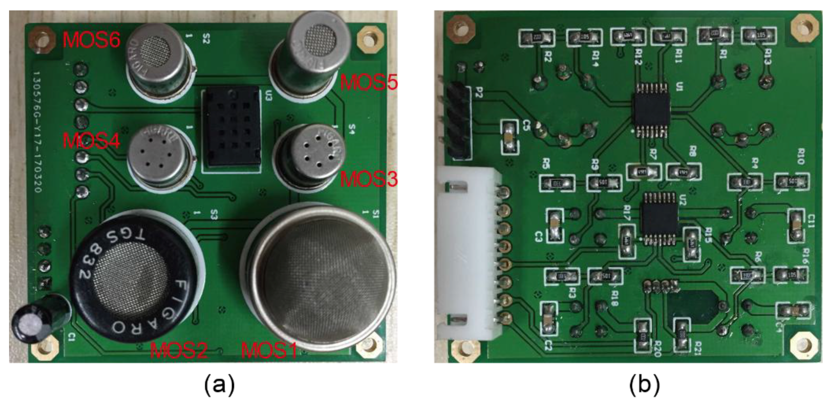
According to the MOS-based sensor principle, the response curve of the sensor to affinity substances quickly rises initially and then gradually flattens. Generally, several kinds of features (e.g., stable value [SV], mean-differential coefficient value, and response area value [
23,
24]), extracted from E-nose signals can be used in pattern recognition algorithms. In this work, we used simpler feature parameters, namely the SV. Because detection lasted for 90 s per sample and the response value of each sensor stabilized after approximately 70 s, as shown in
Figure 4, the value after the 70th second of each sensor was taken as the SV. In this study, the last 10 data points (from the 81st to 90th seconds) were used as input features for model training and testing. Therefore, four datasets used for four group experiments were formed, and datasets were expressed as a 450 × 6 matrix, 600 × 6 matrix, 450 × 6 matrix, or 600 × 6 matrix, respectively.
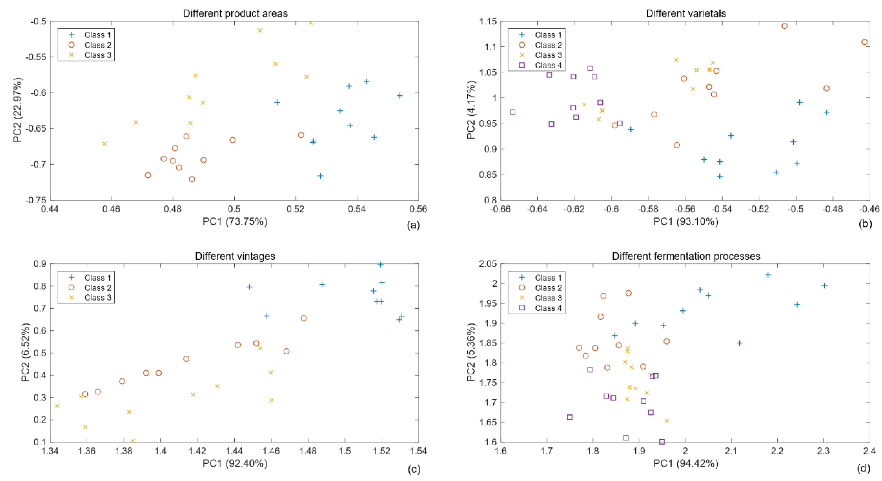
PCA results of four sets of experimental data are presented in
Figure 5, reducing the dimension from six variables to two principal components. The four subplots illustrate that clustering among the various classes is present, but in many cases is highly overlapping. No sets of experimental samples could be easily separated artificially in the new two-dimensional projections space based on PCA. Therefore, we concluded that the odor of wine was strong and rich; in the four sets of experiments, the sample within each group had only one different attribute, and the difference between them was minimal. In PCA, principal components with a small contribution rate were neglected, but it may reflect important differences among sample types. In particular, some useful information was lose after data dimension reduction.
In addition, the loadings plot of PCA is shown in
Figure 6. All six variables (MOS1, …, MOS6) were represented in the subplots by a vector, respectively, and the direction and length of the vector indicate how each variable (sensor) contributes to the two principal components. In the first subplot, the first principal component had positive coefficients for the MOS2, MOS3, and MOS4, and the largest was the MOS4, which showed that MOS4 had the largest contribution to the first principal component in the process of dimension reduction. Similarly, as shown in
Figure 6b–d, the sensor which had the largest contribution to the first principal component was MOS4, MOS5 and MOS5, respectively. It was worth noting that the contribution of the same sensor was different in different tasks. Actually, removing the sensors with low contribution did not improve the experimental performance in this work.
3.3. Comparison of Properties Classification Based on Four Methods
In this work, four methods, namely BPNN, SVM, RF, and XGBoost, were used to classify different properties of wines. The above methods were implemented via PC programming using Python language and Tensorflow (an open source software library for high-performance numerical computation). For ease of comparison, all experimental results (accuracy of the four models in different experiments, respectively) are illustrated in
Table 6, where “Original”, “4-D”, and “2-D” indicate the input features used in models to be original features, 4-dimensional features reduced by PCA, and 2-dimensional features reduced by PCA, respectively.
In BPNN training, several neurons in the hidden layer were explored. During training, three-fold cross-validation was applied to evaluate generalization performance of the BPNN model with final evaluation on the testing set. Taking the first set of experiments as an example, the optimized classification model is shown in
Figure 7. The number of neurons in the hidden layer was determined to be 12. During training, dropout refers to dropping out units (hidden and visible) in a neural network, involving randomly setting the fraction rate of input units to zero at each update to help to prevent overfitting.
In addition, to verify the previous guess (i.e., the contribution of small components containing important information), we compared the performance of original features and dimension-reduced features based on the model we built in each set of experiments. Experimental results are shown in
Table 6. The accuracy of discrimination declined as the feature dimensions decreased. In identifying wine production areas and varietals, BPNN achieved the best performance, with accuracies of 94% and 92.5%, respectively, using original features. Results indicate that BPNN possessed strong nonlinear fitting capabilities in the two classification tasks. Note that, compared to the other methods, the training of BPNN was the most time-consuming (BPNN consumed about three to six seconds, while the others only took tens of milliseconds). Therefore, it seems futile to compare computing time when the input was so small, and we will not discuss training time hereinafter.
For the RF-based classifier model, the main parameters were the number of decision trees and number of features (N
F) in the random subset at each node in the growing trees. During model construction, the number of decision trees was optimized first, after which the N
F was determined. For the number of trees, a larger amount is better but takes longer to compute. Results stop improving substantially beyond a critical number of trees, related to the N
F considered when splitting a node. A lower N
F leads to a greater reduction in variance but larger increase in bias. Only 15 decision trees were used in our experiments to build the classifier model; N
F was defined using the empirical formula mentioned earlier. The performance of RF is also reflected in the
Table 6, revealing that the performance of RF was mediocre in all experiments.
In the SVM-based model, an RBF was chosen as the kernel function. To optimize the penalty parameter (C) and kernel parameter gamma (c) in the SVM model, a grid search method with exponentially growing sequences of C and c was applied. Then, the optimal combination of parameters was determined according to the distinguishability of the computed hyperplane. Finally, four parameter combinations ([C, c]) used for the four tasks were determined to be [10, 0.15], [10, 0.15], [20, 0.1], and [15, 0.1], respectively. According to the experimental results in the
Table 6, SVM achieved the best performance in identifying wine vintage and fermentation processes, with accuracies of 67.3% and 60.5%, respectively.
XGBoost is an efficient implementation of the gradient boosting machine, a representative of ensemble learning. Model parameters were highly similar to those of the RF model, thus, the parameter selection process referenced that of the RF model. Moreover, the experimental results of the XGBoost-based method are also depicted in the
Table 6. It is showed that the XGBoost model did not obtain ideal performance.


