
Estimation of Chlorophyll-a Concentration and the Trophic State of the Barra Bonita Hydroelectric Reservoir Using OLI/Landsat-8 Images

 ,
,
Abstract
:1. Introduction
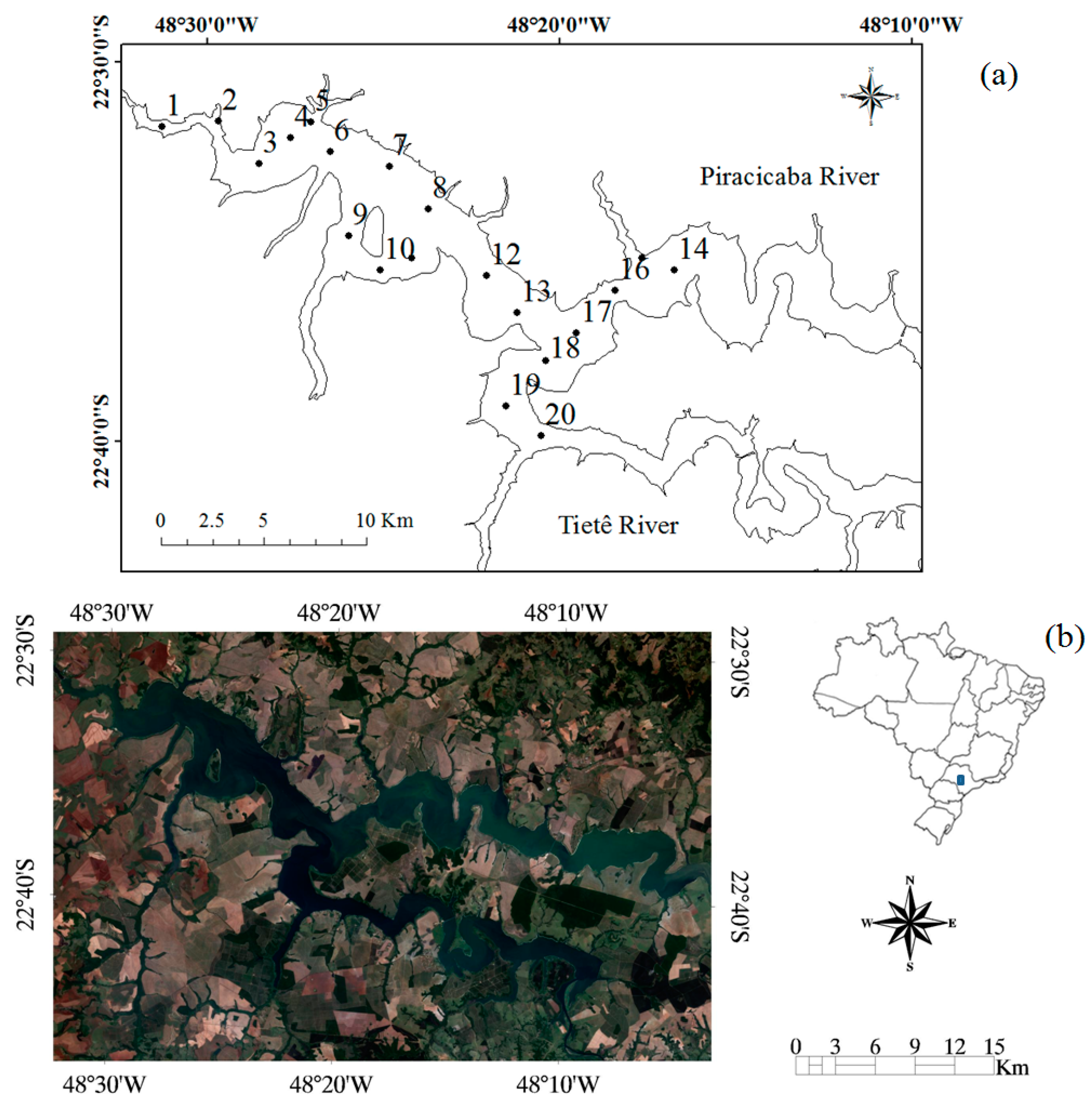
2. Study Area

3. Data and Methods
3.1. Field Survey
Field Measurements
3.2. Laboratory Analysis
3.3. OLI Image Processing
3.4. Model Calibration
3.5. Tuning Models and Application of Existing Models

| Abbreviation | Bands Combination | Reference |
|---|---|---|
| 2B | [70] | |
| 3B | [70] | |
| NDCI | [32] |
| Reference | Index | a * | b * | c * | d * |
|---|---|---|---|---|---|
| [70] | 2B | −37.94 | 61.324 | − | − |
| 3B | 23.174 | 232.29 | − | − | |
| [71] | 2B | −19.3 | 35.75 | − | 1.124 |
| 3B | 16.45 | 113.36 | − | 1.124 | |
| [72] | 2B | −15.18 | 14.85 | 25.28 | − |
| 3B | 25.66 | 215.95 | 315.5 | − | |
| [32] | NDCI | 14.039 | 86.115 | 194.325 | − |
3.6. Validation
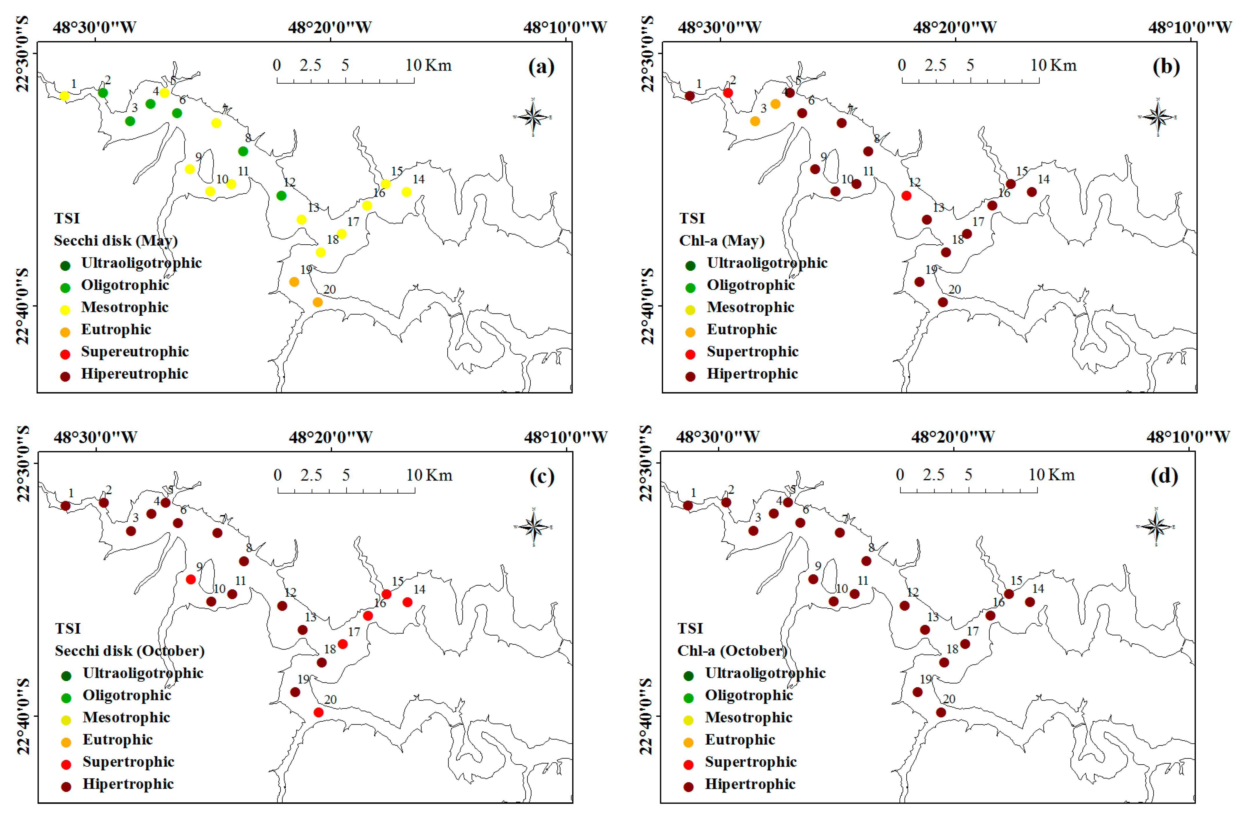
3.7. Trophic State Classification
| Trophic State | Total Phosphorus (mg·L−1) | Chl-a (mg m−3) | Secchi Disk Transparency (m) | TSI |
|---|---|---|---|---|
| Ultraoligotrophic | Pt 0.008 | Chl-a 1.17 | S 2.4 | TSI 47 |
| Oligotrophic | 0.008–0.019 | 1.17–3.24 | 2.4–1.7 | 47–52 |
| Mesotrophic | 0.019–0.052 | 3.24–11.03 | 1.7–1.1 | 52–59 |
| Eutrophic | 0.052–0.12 | 11.03–30.55 | 1.1–0.8 | 59–63 |
| Supertrophic | 0.12–0.2333 | 30.55–69.05 | 0.8–0.6 | 63–67 |
| Hypertrophic | 0.233 < Pt | 69.05 < Chl-a | 0.6 > S | TSI > 67 |
4. Results

| a. Dataset measured on 5–9 May 2014 at 19 stations | ||||||
| Parameter | Min | Max | Mean | Median | SD | CV (%) |
| Chl-a, mg m−3 | 19.1 | 293.2 | 122.5 | 105.9 | 72.3 | 60 |
| Secchi disk depth, m | 0.8 | 2.3 | 1.5 | 1.4 | 0.4 | 30 |
| Turbidity, NTU | 1.7 | 12.5 | 5.2 | 5 | 2.5 | 50 |
| TSS, mg L−1 | 3.6 | 16.3 | 7.0 | 6.5 | 3.2 | 50 |
| OSS, mg L−1 | 2.8 | 14.7 | 5.9 | 4.8 | 3.1 | 50 |
| ISS, mg L−1 | 0.2 | 4.4 | 1.1 | 0.8 | 0.9 | 80 |
| OSS/TSS | 0.45 | 0.98 | 0.83 | 86 | 11.6 | 10 |
| ISS/TSS | 0.02 | 0.55 | 0.17 | 14 | 11.6 | 70 |
| aphy (665), m−1 | 0.2 | 1.3 | 0.6 | 0.5 | 0.3 | 50 |
| aCDOM (440), m−1 | 0.6 | 1.1 | 0.8 | 0.8 | 0.1 | 10 |
| ap (440), m−1 | 0.7 | 2.9 | 1.6 | 1.5 | 0.7 | 40 |
| Wind, m s−1 | 0.6 | 4.9 | 1.8 | 1.6 | 1.1 | 60 |
| b. Dataset measured on 13–16 October 2014 at 20 stations | ||||||
| Parameter | Min | Max | Mean | Median | SD | CV(%) |
| Chl-a, mg m−3 | 263.2 | 797.8 | 428.7 | 368.9 | 154.5 | 40 |
| Secchi disk depth, m | 0.4 | 0.8 | 0.6 | 0.6 | 0.1 | 20 |
| Turbidity, NTU | 11.6 | 33.2 | 18.6 | 17.6 | 5.3 | 30 |
| TSS, mg L−1 | 10.8 | 44 | 22 | 21.2 | 7 | 30 |
| OSS, mg L−1 | 10.2 | 30.4 | 18.2 | 18.4 | 4.8 | 30 |
| ISS, mg L−1 | 0.6 | 3.8 | 2.6 | 2.8 | 1 | 40 |
| OSS/TSS | 0.8 | 1 | 0.9 | 0.9 | 0.1 | 10 |
| ISS/TSS | 0.04 | 0.2 | 0.1 | 0.1 | 0.4 | 10 |
| aphy (665), m−1 | 0.6 | 2.1 | 1.1 | 1 | 0.4 | 40 |
| aCDOM (440), m−1 | 0.9 | 2.4 | 1.3 | 1.3 | 0.3 | 30 |
| ap (440), m−1 | 1.6 | 5.6 | 2.8 | 2.6 | 1 | 40 |
| Wind, m s−1 | 0 | 5 | 1.5 | 1.1 | 1.5 | 100 |


| Index | a | b | c | R2 | p-value |
|---|---|---|---|---|---|
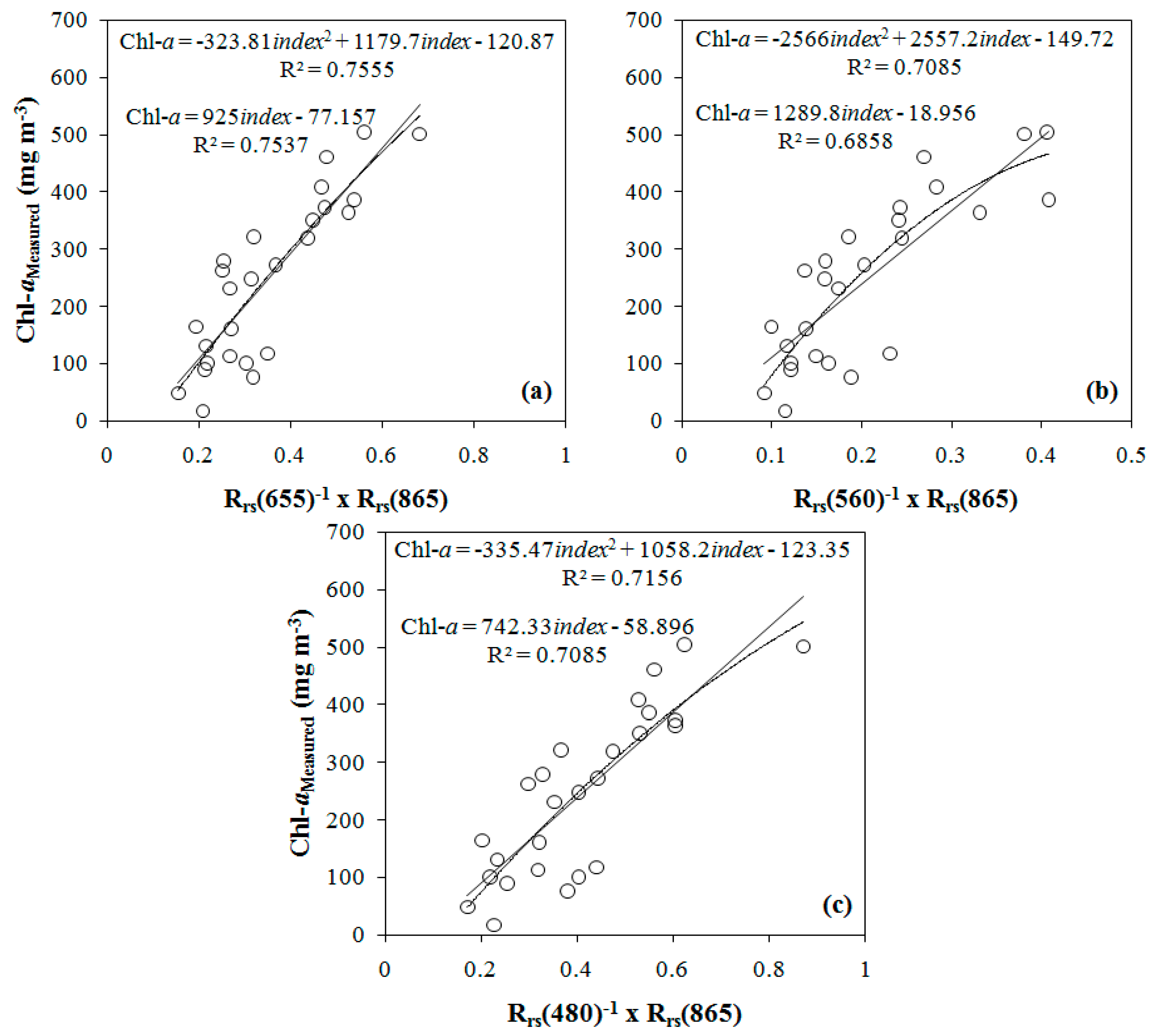
| NIR/Red (Linear) | −77.16 | 925.001 | − | 0.7537 | 0.00000 |
| NIR/Green (Linear) | −18.96 | 1289.84 | − | 0.6858 | 0.00000 |
| NIR/Blue (Linear) | −58.90 | 742.33 | − | 0.7085 | 0.00000 |
| NIR/Red (Polynomial) | −120.87 | 1179.72 | −323.81 | 0.7555 | 0.00000 |
| NIR/Green (Polynomial) | −149.72 | 2557.24 | −2565.99 | 0.7085 | 0.00000 |
| NIR/Blue (Polynomial) | −123.35 | 1058.23 | −335.47 | 0.7156 | 0.00000 |
| 2B (Linear) | −124.72 | 213.73 | − | 0.3910 | 0.0006 |
| 3B (Linear) | 71.212 | 603.15 | − | 0.5794 | 0.00001 |
| NDCI (Linear) | 53.361 | 767.2 | - | 0.3945 | 0.0006 |
| 2B (Polynomial) | −214.41 | 321.62 | −30.63 | 0.3926 | 0.0006 |
| 3B (Polynomial) | 33.95 | 918.36 | −465.68 | 0.5963 | 0.00001 |
| NDCI (Polynomial) | 56.818 | 724.88 | 93.472 | 0.3946 | 0.0006 |
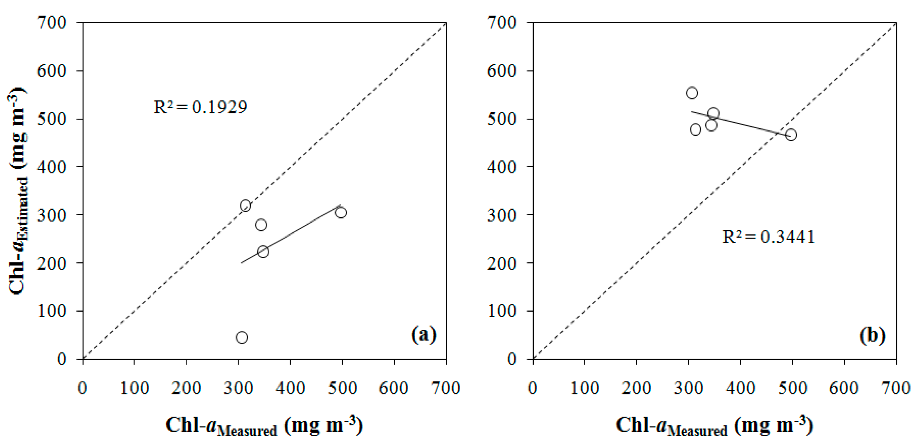
| a. Models calibrated using ICE [62] from OLI bands simulated and data collected in the study area. | ||||||
| Model | NRMSE (%) | MAPE (%) | Bias | MNB (%) | NRMS (%) | R2 |
| NIR/Red (Linear) | 170.01 | 91.96 | 307.56 | 91.96 | 44.17 | 0.1921 |
| NIR/Green (Linear) | 190.91 | 103.90 | 348.61 | 103.90 | 47.00 | 0.2823 |
| NIR/Blue (Linear) | 100.78 | 52.32 | 163.16 | 50.84 | 36.12 | 0.3301 |
| NIR/Red (Polynomial) | 144.17 | 77.92 | 259.62 | 77.92 | 37.71 | 0.1934 |
| NIR/Green (Polynomial) | 82.39 | 36.02 | −126.47 | −35.13 | 32.38 | 0.1929 |
| NIR/Blue (Polynomial) | 86.54 | 45.69 | 137.90 | 43.28 | 31.47 | 0.3441 |
| b. Tuning bands combinations proposed by literature. | ||||||
| Model | NRMSE (%) | MAPE (%) | Bias | MNB (%) | NRMS (%) | R2 |
| 2B (Linear) | 32.09 | 13.60 | −51.71 | −13.60 | 8.39 | 0.816 |
| 3B (Linear) | 18.70 | 8.90 | 0.75 | −0.47 | 11.62 | 0.7953 |
| NDCI (Linear) | 33.84 | 12.48 | −49.56 | −12.44 | 9.59 | 0.867 |
| 2B (Polynomial) | 32.49 | 12.96 | −50.26 | −12.96 | 8.86 | 0.7918 |
| 3B (Polynomial) | 16.72 | 7.67 | −3.19 | −0.34 | 9.69 | 0.7724 |
| NDCI (Polynomial) | 33.57 | 12.48 | −49.54 | −12.48 | 9.47 | 0.7759 |
| c. Models proposed by authors, calibrated using data from other environments | ||||||
| Model | NRMSE (%) | MAPE (%) | Bias | MNB (%) | NRMS (%) | R2 |
| 2B [70] | 146.82 | 75.82 | −274.69 | −75.82 | 2.35 | 0.816 |
| 3B [70] | 120.13 | 62.88 | −226.17 | −62.88 | 4.56 | 0.867 |
| 2B [71] | 146.19 | 75.64 | −273.87 | −75.64 | 2.37 | 0.821 |
| 3B [71] | 127.51 | 66.81 | −240.23 | −66.81 | 4.35 | 0.8723 |
| 2B [72] | 128.11 | 66.68 | −240.63 | −66.68 | 3.84 | 0.841 |
| 3B [72] | 80.45 | 43.57 | −151.14 | −43.57 | 13.62 | 0.8975 |
| NDCI [32] | 157.99 | 81.72 | −295.85 | −81.72 | 1.85 | 0.7978 |


5. Discussion
6. Conclusions
Acknowledgments
Author Contributions
Conflicts of Interest
References
- Liu, Y.; Islam, M.A.; Gao, J. Quantification of shallow waters quality parameters by means of remote sensing. Prog. Phys. Geogr. 2003, 27, 111–117. [Google Scholar] [CrossRef]
- Calijuri, M.C.; Santos, A.C.A.; Jati, S. Temporal changes in the phytoplankton community structure in a tropical and eutrophic reservoir (Barra Bonita, S.P.–Brazil). J. Plankton Res. 2002, 24, 617–634. [Google Scholar] [CrossRef]
- Smith, V.H. Eutrophication of freshwater and coastal marine ecosystems: a global problem. Environ. Sci. Pollut. 2003, 10, 126–139. [Google Scholar] [CrossRef]
- Bennett, E.M.; Carpenter, S.R.; Caraco, N.F. Human impact on erodable phosphorus and eutrophication: a global perspective. BioScience 2001, 51, 227–234. [Google Scholar] [CrossRef]
- Cai, W.J.; Hu, X.; Huang, W.J.; Murrel, M.C.; Lehrter, J.C.; Lohrens, S.E.; Chou, W.C.; Zhai, W.; Hollibaugh, J.T.; Wang, Y.; et al. Acidification of subsurface coastal waters enhanced by eutrophication. Nat. Geosci. 2011, 4, 766–770. [Google Scholar] [CrossRef]
- Rabalais, N.N.; Turner, R.E.; Díaz, R.J.; Justic, D. Global change and eutrophication of coastal waters. ICES J. Marine Sci. 2009, 66, 1528–1537. [Google Scholar] [CrossRef]
- Smith, V.H. Cultural eutrophication of inland, estuarine and coastal waters. In Successes, Limitations and Frontiers in Ecosystems Science; Pace, M.L., Groffman, P.M., Eds.; Springer-Verlag: New York, NY, USA, 1998; pp. 7–49. [Google Scholar]
- Blain, S.; Quéguiner, B.; Armand, L.; Belviso, S.; Bombled, B.; Bopp, L.; Bowie, A.; Brunet, C.; Brussaard, C.; Carlotti, F.; et al. Effect of natural iron fertilization on carbon sequestration in the Southern Ocean. Nature 2007, 446, 1070–1075. [Google Scholar] [CrossRef] [PubMed]
- Boyd, P.W.; Jickells, T.; Law, C.S.; Blain, S.; Boyle, E.A.; Buesseler, K.O.; Coale, K.H.; Cullen, J.J.; Baar, H.J.W.; Follows, M.; et al. Mesoscale iron enrichment experiments 1993–2005 synthesis and future directions. Science 2007, 315, 612–617. [Google Scholar] [CrossRef] [PubMed]
- Sayre, R. Microalgae: The potential for carbon capture. BioScience 2010, 60, 722–272. [Google Scholar] [CrossRef]
- Giles, J. Methane quashes green credentials of hydropower. Nature 2006, 444, 524–525. [Google Scholar] [CrossRef] [PubMed]
- Abe, D.S.; Matsumura-Tundisi, T.; Rocha, O.; Tundisi, J.G. Denitrification and bacterial community structure in the cascade of six reservoirs on a tropical river in Brazil. Hydrological 2003, 504, 67–76. [Google Scholar] [CrossRef]
- Roland, F.; Vidal, L.O.; Pacheco, F.S.; Barros, N.O.; Assireu, A.; Ometto, J.P.H.B.; Cimbleris, A.C.P.; Cole, J.J. Variability of carbon dioxide flux from tropical (Cerrado) hydroeletric reservoirs. Aquat. Sci. 2010, 72, 283–293. [Google Scholar] [CrossRef]
- Kemenes, A.; Forsberg, B.R.; Melack, J.M. CO2 emissions from a tropical hydroeletric reservoir (Balbina, Brazil). J. Geophys. Res. 2011, 116. [Google Scholar] [CrossRef]
- Barros, N.; Cole, J.J.; Tranvik, L.J.; Prairie, Y.T.; Bastviken, D.; Huszar, V.L.M.; Giorgio, P.; Roland, F. Carbon emission from hydroelectric reservoirs linked to reservoir age and latitude. Nat. Geosci. 2011, 4, 593–596. [Google Scholar] [CrossRef]
- Weaver, E.C.; Wrigley, R. Factors Affecting the Identification of Phytoplankton Groups by Means of Remote Sensing; NASA Ames Research Center: Moffett Field, CA, USA, 1994. [Google Scholar]
- Pearson, L.; Mihali, T.; Moffit, M.; Kellmann, R.; Neilan, B. On the chemistry, toxicology and genetics of the cyanobacterial toxins, microcystin, nodularin, saxitoxin and cylindrospermopsin. Mar. Drugs. 2010, 8, 1650–1680. [Google Scholar] [CrossRef] [PubMed]
- Neilan, B.A.; Dittmann, E.; Rouhiainen, L.; Bass, R.A.; Schaub, V.; Sivonen, K.; Börner, T. Nonribosomal peptide synthesis and tosigenicity of cyanobacteria. J. Bacteriol. 1999, 181, 4089–4097. [Google Scholar] [PubMed]
- McGregor, G.B.; Stewart, I.; Sendall, B.C.; Sadler, R.; Reardon, K.; Carter, S.; Wruck, D.; Wickramasinghe, W. First report of a toxic Nodularia spumigena (Nostocales/Cyanobateria) blooms in sub-tropical Australia. I. Phycological and public health investigations. Int. J. Environ. Res. Public Health 2012, 9, 2396–2411. [Google Scholar] [CrossRef] [PubMed]
- Ju, J.; Saul, N.; Kochan, C.; Putschew, A.; Pu, Y.; Yiu, L.; Steinberg, C.E.W. Cyanobaterial xenobiotcs as evaluated by a Caenorhabditis elegans neurotoxicity screening test. Int. J. Environ. Res. Public Health. 2014, 11, 4589–4606. [Google Scholar] [CrossRef] [PubMed]
- Carlson, R.E. A trophic state index for lakes. Limnol. Oceanogr. 1977, 22, 361–369. [Google Scholar] [CrossRef]
- Walker, W.W. Predicting lake water quality. In The lake and reservoir restoration guidance manual, 1st ed.; Lynn, M., Kent, T., Eds.; EPA: Washington, DC, USA, 1998; pp. 1–23. [Google Scholar]
- Lamparelli, M.C. Graus de trofia em corpos d’água do Estado de São Paulo. Ph.D. Thesis, University of São Paulo, State of São Paulo, Brazil, 3 Sepetmber 2004. [Google Scholar]
- Palmer, S.C.J.; Kutser, T.; Hunter, P.D. Remote sensing of inland waters: Challenges, progress and future directions. Remote Sens. Environ. 2015, 157, 1–8. [Google Scholar] [CrossRef]
- Koponen, S.; Pullainen, J.; Kallio, K.; Hallikainen, M. Lake water quality classification with airborne hyperspectral spectrometer and simulated MERIS data. Remote Sens. Environ. 2002, 79, 51–59. [Google Scholar] [CrossRef]
- Kirk, J.T.O. Light and Photosynthesis in Aquatic Ecosystems, 3rd ed.; Cambridge University Press: Cambridge, UK, 2011. [Google Scholar]
- Bukata, R.P.; Jerome, J.H.; Kondratyev, K.Y.; Pozdnyakov, D.V. Optical Properties and Remote Sensing of Inland and Coastal Waters; CRC Press: Boca Raton, FL, USA, 1995. [Google Scholar]
- Carder, K.L.; Chen, F.R.; Lee, Z.P.; Hawes, S.K.; Kamykowski, D. Semianalytic Moderate-Resolution Imaging Spectrometer algorithms for chlorophyll a and absorption with bio-optical domains based on nitrate-depletion temperatures. J. Geophys. Res. 1999, 104, 5403–5421. [Google Scholar] [CrossRef]
- Brando, V.E.; Dekker, A.G. Satellite hyperspectral remote sensing for estimating estuarine and coastal water quality. IEEE Trans. Geosci. Remote Sens. 2003, 41, 1378–1387. [Google Scholar] [CrossRef]
- Doeffer, R.; Schiller, H. The MERIS Case 2 water algorithm. Int. J. Remote Sens. 2007, 28, 517–535. [Google Scholar] [CrossRef]
- Gitelson, A.A.; Schalles, J.F.; Hladik, C.M. Remote chlorophyll-a retrieval in turbid, productive estuaries: Chesapeake Bay case study. Remote Sens. Environ. 2007, 109, 464–472. [Google Scholar] [CrossRef]
- Mishra, S.; Mishra, D.R. Normalized difference chlorophyll index: A novel model for remote estimation of chlorophyll-a concentration in turbid productive waters. Remote Sens. Environ. 2012, 117, 394–406. [Google Scholar] [CrossRef]
- Huang, C.; Zou, J.; Li, Y.; Yang, H.; Shi, K.; Li, J.; Wang, Y.; Chena, X.; Zheng, F. Assessment of NIR-red algorithms for observation of chlorophyll-a in highly turbid inland waters in China. ISPRS J. Photogramm. 2014, 93, 29–39. [Google Scholar] [CrossRef]
- Matsushita, B.; Yang, W.; Yu, G.; Oyama, Y.; Yoshimura, K.; Fukushima, T. A hybrid algorithm for estimating the chlorophyll-a concentration across different trophic states in Asian inland waters. ISPRS J. Photogramm. Remote Sens. 2015, 102, 28–37. [Google Scholar] [CrossRef]
- Mayo, M.; Gitelson, A.; Yacobi, Y.Z.; Ben-Avraham, Z. Chlorophyll distribution in Lake Kinneret determined from Landsat Thematic Mapper data. Int. J. Remote Sens. 1995, 16, 175–182. [Google Scholar] [CrossRef]
- Yacobi, Y.Z.; Gitelson, A.; Mayo, M. Remote sensing of chlorophyll in Lale Kinneret using higj spectral-resolution radiometer and Landsat TM: Spectral features of reflectance and algorithm development. J. Plankton Res. 1995, 117, 2155–2173. [Google Scholar] [CrossRef]
- Vincent, R.K.; Qin, X.; McKay, M.L.; Miner, J.; Czajkowski, K.; Savino, J.; Bridgeman, T. Phycocyanin detection from LANDSAT TM data for mapping cyanobacterial blooms in Lake Erie. Remote. Sens. Environ. 2004, 89, 381–392. [Google Scholar] [CrossRef]
- Sun, D.; Hu, C.; Qiu, Z.; Shi, K. Estimating phycocyanin pigment concentration in productive inland waters using Landsat measurements: A case study in Lake Dianchi. Opt. Express. 2015, 23, 3055–3074. [Google Scholar] [CrossRef] [PubMed]
- Thiemann, S.; Kaufmann, H. Determination of chlorophyll content and trophic state of lakes using field spectrometer and IRS-1C satellite data in the Mecklenburg Lake District, Germany. Remote Sens. Environ. 2000, 73, 227–235. [Google Scholar] [CrossRef]
- Pahlevan, N.; Lee, Z.-P.; Wei, J.; Schaaf, C.B.; Schott, J.R.; Berk, A. On-orbit radiometric characterization of OLI (Landsat-8) for applications in aquatic remote sensing. Remote Sens. Environ. 2014, 154, 272–284. [Google Scholar] [CrossRef]
- Vanhellemont, Q.; Ruddick, K. Turbid wakes associated with offshore wind turbines observed with Landsat 8. Remote Sens. Environ. 2014, 145, 105–115. [Google Scholar] [CrossRef]
- Lobo, F.L.; Costa, A.P.F.; Novo, E.M.L.M. Time-series analysis of Landsat-MSS/TM/OLI images over Amazonian waters impacted by gold mining activities. Remote Sens. Environ. 2015, 157, 170–184. [Google Scholar] [CrossRef]
- CETESB (Companhia Ambiental do Estado de São Paulo). Águas superficiais. CETESB: São Paulo, Brasil. Available online: http://www.cetesb.sp.gov.br/agua/aguas-superficiais/35-publicacoes-/-relatorios (accessed on 23 April 2015).
- Tundisi, J.G.; Matsumura-Tundisi, T.; Abe, D.S. The ecological dynamics of Barra Bonita (Tietê River, SP, Brazil) reservoir: Implications for its biodiversity. Brazilian J. Biol. 2008, 68, 1079–1098. [Google Scholar] [CrossRef]
- AES Tietê. Barra Bonita. 2013. Available online: http://www.aestiete.com.br/usinas/Paginas/BarraBonita.aspx\ (accessed on 19 May 2015).
- Matsumura-Tundisi, T.; Tundisi, J.G. Plankton richness in a eutrophic reservoir (Barra Bonita reservoir, SP, Brazil). Hydrobiologia 2005, 542, 367–378. [Google Scholar] [CrossRef]
- Calijuri, M.C.; Santos, A.C.A. Short-term changes in the Barra Bonita reservoir (São Paulo, Brazil): Emphasis on the phytoplankton communities. Hydrobiologia 1996, 330, 163–175. [Google Scholar] [CrossRef]
- Dellamano-Oliveira, M.J.; Vieira, A.A.H.; Rocha, O.; Colombo, V. Phytoplankton taxonomic composition and temporal changes in a tropical reservoir. Funda. Appl. Limnol. 2008, 171, 27–38. [Google Scholar] [CrossRef]
- Rodrigues, T.W.P.; Guimarães, U.S.; Rotta, L.H.S.; Watanabe, F.S.Y.; Alcântara, E.; Imai, N.N. Delineamento amostral em reservatórios utilizando imagens Landsat-8/OLI: um estudo de caso no reservatório de Nova Avanhandava (Estado de São Paulo, Brasil). Boletim de Ciências Geodésicas 2015. submitted. [Google Scholar]
- msda_xe—Analysis and Control Software. Available online: http://trios-science.com/index.php?option=com_content&view=article&id=104&catid=65&Itemid=91&lang=en (accessed on 26 June 2015).
- Mobley, C.D. Estimation of the remote-sensing reflectance from above-surface measurements. Appl. Opt. 1999, 38, 7442–7455. [Google Scholar] [CrossRef] [PubMed]
- Mueller, J.L. In-water radiometric profile measurements and data analysis protocols. In Ocean Optics Protocols for Satellite Ocean Color Sensor Validation, Revision 4, Volume III: Radiometric Measurements and Data Analysis Protocols; Muller, J.L., Fargion, G.S., McClain, C.R., Eds.; NASA Goddard Space Flight Space Center: Greenbelt, MD, USA, 2003; pp. 7–20. [Google Scholar]
- Golterman, H.L. Developments in Water Science 2. In Physiological Limnology: An Approach to the Physiology of Lake Ecosystems; Elsevier: Amsterdam, The Netherlands, 1975. [Google Scholar]
- APHA. Standard Methods for the Examination of Water and Wastewater, 20th ed.; American Public Health Association (APHA), American Water Works Association (AWWA), Water Environmental Federation (WEF): Washintong, DC, USA, 1998. [Google Scholar]
- Cleveland, J.S.; Weidemann, A.D. Quantifying absorption by aquatic particles: A multiple scattering correction for glass-fiber filters. Limnol. Oceanogr. 1993, 38, 1321–1327. [Google Scholar] [CrossRef]
- Tassan, S.; Ferrari, G.M. Measurement of light absorption by aquatic particles retained on filters: Determination of the optical pathlength amplification by the “transmittance-reflectance” method. J. Plankton Res. 1998, 20, 1699–1709. [Google Scholar] [CrossRef]
- Bricaud, A.; Morel, A.; Prieur, L. Absorption by dissolved organic matter of the sea (yellow substance) in the UV and visible domains. Limnol. Oceanogr. 1981, 26, 43–53. [Google Scholar] [CrossRef]
- Frequently Asked Questions About the Landsat Missions. Available online: landsat.usgs.gov/best_spectral_bands_to_use.php (accessed on 23 April 2015).
- Atmospheric Correction Module: QUAC and FLAASH User’s Guide. Available online: https://www.exelisvis.com/portals/0/pdfs/envi/Flaash_Module.pdf (accessd on 26 June 2015).
- Aerosols and Climate Change. Available online: http://earthobservatory.nasa.gov/Features/Aerosols/what_are_aerosols_1999.pdf (accessed on 29 July 2015).
- Mishra, D.R.; Narumalani, S.; Rundquist, D.; Lawson, M. Characterizing the vertical diffuse attenuation coefficient for downwelling irradiance in coastal waters: Implications for water penetration by high resolution satellite data. ISPRS J. Photogramm. 2005, 60, 48–64. [Google Scholar] [CrossRef]
- Gordon, H.R.; Brown, J.W.; Evans, R.H. Exact Rayleigh scattering calculations for use with the Nimbus-7 Coastal Zone Color Scanner. Appl. Opt. 1988, 27, 862–871. [Google Scholar] [CrossRef] [PubMed]
- Ruddick, K.G.; Ovidio, F.; Rijkeboer, M. Atmospheric correction of SeaWiFS imagery for turbid coastal and inland waters. Appl. Opt. 2000, 39, 897–912. [Google Scholar] [CrossRef] [PubMed]
- Vanhellemont, Q.; Ruddick, K. Advantages of high quality SWIR bands for ocean colour processing: Examples from Landsat-8. Remote Sens. Environ. 2015, 161, 89–106. [Google Scholar] [CrossRef]
- Moses, J.M.; Gitelson, A.A.; Perk, R.L.; Gurlin, D.; Rundquist, D.C.; Leavitt, B.C.; Barrow, T.M.; Brakhage, P. Estimation of chlorophyll-a concentration in turbid productive waters using airborne hyperspectral data. Water Res. 2012, 46, 993–1004. [Google Scholar] [CrossRef] [PubMed]
- Moses, W.J.; Bowles, J.H.; Corson, M.R. Expected improvements in the quantitative remote sensing of optically complex waters with the use of an optically fast hyperspectral spectrometer—A modeling study. Sensors 2015, 15, 6152–6173. [Google Scholar] [CrossRef] [PubMed]
- Gitelson, A.A.; Gritz, Y.; Merzlyak, M.N. Relationships between leaf chlorophyll content and spectral reflectance and algorithms for non-destructive chlorophyll assessment in higher plant leaves. J. Plant Physiol. 2003, 160, 271–282. [Google Scholar] [CrossRef] [PubMed]
- Barsi, J.A.; Lee, K.; Kvaran, G.; Markham, B.L.; Pedelyy, J. The spectral response of the Landsat-8 Operational Land Imager. Remote Sens. 2014, 6, 1023–1025. [Google Scholar] [CrossRef]
- Ogashawara, I.; Curtarelli, M.P.; Souza, A.F.; Augusto-Silva, P.B.; Alcântara, E.H.; Stech, J.L. Interactive Correlation Environment (ICE)—A statistical web tool for data collinearity analysis. Remote Sens. 2014, 6, 3059–3074. [Google Scholar] [CrossRef]
- Moses, W.J.; Gitelson, A.A.; Berdnikov, S.; Povazhnyy, V. Satellite estimation of chlorophyll-a concentration using the red and NIR bands of MERIS–the Azov Sea case study. IEEE Geosci. Remote S. 2009, 6, 845–849. [Google Scholar] [CrossRef]
- Gilerson, A.A.; Gitelson, A.A.; Zhou, J.; Gurlin, D.; Moses, W.; Ioannou, I.; Ahmed, S.A. Algorithms for remote estimation of chlorophyll-a in coastal and inland waters using red and near infrared bands. Opt. Express 2010, 18, 109–125. [Google Scholar] [CrossRef] [PubMed]
- Gurlin, D.; Gitelson, A.A.; Moses, W.J. Remote sensing of chl-a concentration in turbid productive waters—Return to a simple two-band NIR-red model? Remote Sens. Environ. 2011, 115, 3479–3490. [Google Scholar] [CrossRef]
- Rundquist, D.C.; Han, L.; Schalles, J.F.; Peake, J.S. Remote measurement of algal chlorophyll in surface waters: The case for the first derivative of reflectance near 690 nm. Photogramm. Eng. Remote Sensing 1996, 62, 195–200. [Google Scholar]
- Detection of Optical Water Quality Parameter for Eutrophic Water by High Resolution Remote Sensing. Available online: http://dspace.ubvu.vu.nl/handle/1871/12714 (accessed on 26 June 2015).
- Soares, A.; Mozeto, A.A. Water quality in the Tietê river reservoirs (Billings, Barra Bonita, Bariri and Promissão, SP-Brazil) and nutrient fluxes across the sediment-water interface (Barra Bonita). Acta Limnol. Bras. 2006, 18, 247–266. [Google Scholar]
- Carlson, R.E. More complications in the chlorophyll-secchi disk relationship. Limnol. Oceanogr. 1980, 25, 379–382. [Google Scholar] [CrossRef]
- Lorenzen, M.W. Use of chlorophyll-Secchi disk relationships. Limnol. Oceanogr. 1980, 25, 371–372. [Google Scholar] [CrossRef]
- Megard, R.O.; Settles, J.C.; Boyer, H.A. Light, Secchi disk, and trophic states. Limnol. Oceanogr. 1980, 25, 373–377. [Google Scholar] [CrossRef]
- Mannino, A.; Russ, M.E.; Hooker, S.B. Algorithms development and validation for satellite-derived distributions of DOC and CDOM in the U.S. Middle Atlantic Bight. J. Geophys. Res. 2008, 13. [Google Scholar] [CrossRef]
© 2015 by the authors; licensee MDPI, Basel, Switzerland. This article is an open access article distributed under the terms and conditions of the Creative Commons Attribution license (http://creativecommons.org/licenses/by/4.0/).
Share and Cite
Watanabe, F.S.Y.; Alcântara, E.; Rodrigues, T.W.P.; Imai, N.N.; Barbosa, C.C.F.; Rotta, L.H.d.S. Estimation of Chlorophyll-a Concentration and the Trophic State of the Barra Bonita Hydroelectric Reservoir Using OLI/Landsat-8 Images. Int. J. Environ. Res. Public Health 2015, 12, 10391-10417. https://doi.org/10.3390/ijerph120910391
Watanabe FSY, Alcântara E, Rodrigues TWP, Imai NN, Barbosa CCF, Rotta LHdS. Estimation of Chlorophyll-a Concentration and the Trophic State of the Barra Bonita Hydroelectric Reservoir Using OLI/Landsat-8 Images. International Journal of Environmental Research and Public Health. 2015; 12(9):10391-10417. https://doi.org/10.3390/ijerph120910391
Chicago/Turabian StyleWatanabe, Fernanda Sayuri Yoshino, Enner Alcântara, Thanan Walesza Pequeno Rodrigues, Nilton Nobuhiro Imai, Cláudio Clemente Faria Barbosa, and Luiz Henrique da Silva Rotta. 2015. "Estimation of Chlorophyll-a Concentration and the Trophic State of the Barra Bonita Hydroelectric Reservoir Using OLI/Landsat-8 Images" International Journal of Environmental Research and Public Health 12, no. 9: 10391-10417. https://doi.org/10.3390/ijerph120910391
APA StyleWatanabe, F. S. Y., Alcântara, E., Rodrigues, T. W. P., Imai, N. N., Barbosa, C. C. F., & Rotta, L. H. d. S. (2015). Estimation of Chlorophyll-a Concentration and the Trophic State of the Barra Bonita Hydroelectric Reservoir Using OLI/Landsat-8 Images. International Journal of Environmental Research and Public Health, 12(9), 10391-10417. https://doi.org/10.3390/ijerph120910391