Convergence and Stability Improvement of Quasi-Newton Methods by Full-Rank Update of the Jacobian Approximates

Abstract

A system of simultaneous multi-variable nonlinear equations can be solved by Newton’s method with local q-quadratic convergence if the Jacobian is analytically available. If this is not the case, then quasi-Newton methods with local q-superlinear convergence give solutions by approximating the Jacobian in some way. Unfortunately, the quasi-Newton condition (Secant equation) does not completely specify the Jacobian approximate in multi-dimensional cases, so its full-rank update is not possible with classic variants of the method. The suggested new iteration strategy (“T-Secant”) allows for a full-rank update of the Jacobian approximate in each iteration by determining two independent approximates for the solution. They are used to generate a set of new independent trial approximates; then, the Jacobian approximate can be fully updated. It is shown that the T-Secant approximate is in the vicinity of the classic quasi-Newton approximate, providing that the solution is evenly surrounded by the new trial approximates. The suggested procedure increases the superlinear convergence of the Secant method $\left({\phi }_S=1.618\dots \right)$ to super-quadratic $\left({\phi }_T={\phi }_S+1=2.618\dots \right)$ and the quadratic convergence of the Newton method $\left({\phi }_N=2\right)$ to cubic $\left({\phi }_T={\phi }_N+1=3\right)$ in one-dimensional cases. In multi-dimensional cases, the Broyden-type efficiency (mean convergence rate) of the suggested method is an order higher than the efficiency of other classic low-rank-update quasi-Newton methods, as shown by numerical examples on a Rosenbrock-type test function with up to 1000 variables. The geometrical representation (hyperbolic approximation) in single-variable cases helps explain the basic operations, and a vector-space description is also given in multi-variable cases.

1. Introduction

It is a common task in numerous disciplines (e.g., physics, chemistry, biology, economics, robotics, and engineering, social, and medical sciences) to construct a mathematical model with some parameters for an observed system which gives an observable response to an observable external effect. The unknown parameters of the mathematical model are determined so that the difference between the observed and the simulated system responses of the mathematical model for the same external effect is minimized (see e.g., [1,2,3,4,5,6,7,8,9,10,11]). This problem leads to finding the zero of a residual function (difference between observed and simulated responses). The rapidly accelerating computational tools and the increasing complexity of mathematical models with more and more efficient numerical algorithms provide a chance for better understanding and control of the surrounding nature.

As referenced above, root-finding methods are essential for solving a great class of numerical problems, such as data fitting problems with $\mathit{m}$ sampled data $\mathit{D}=\left[{\mathit{D}}_{\mathit{j}}\right]$ ($\mathit{j}=1,\dots ,\mathit{m}$) and $\mathit{n}$ adjustable parameters $\mathit{x}=\left[{\mathit{x}}_{\mathit{i}}\right]$ ($\mathit{i}=1,\dots ,\mathit{n}$) with $\mathit{m}\ge \mathit{n}$. This leads to the problem of least-squares solving of an over-determined system of nonlinear equations,

$$\mathit{f}\left(\mathit{x}\right)=\mathbf{0},$$

(1)

($\mathit{x}\in$${\mathbb{R}}^{\mathit{n}}$ and $\mathit{f}:{\mathbb{R}}^n\to {\mathbb{R}}^m$ ($m\ge n$)), where the solution ${\mathit{x}}^{*}$ minimizes the difference

$${∥\mathit{f}\left(\mathit{x}\right)∥}_2={∥\varphi \left(\mathit{x}\right)-\mathit{D}∥}_{\mathit{2}}$$

(2)

between the data $\mathit{D}$ and a computational model function $\varphi \left(\mathit{x}\right)$. The system of simultaneous multi-variable nonlinear Equation (1) can be solved by Newton’s method when the derivatives of $\mathit{f}\left(\mathit{x}\right)$ are available analytically and a new iterate,

$${\mathit{x}}_{p+1}={\mathit{x}}_p-{\mathit{J}}_p^{-1}{\mathit{f}}_p,$$

(3)

that follows ${\mathit{x}}_p$ can be determined, where ${\mathit{f}}_p=\mathit{f}\left({\mathit{x}}_p\right)$ is the function value and ${\mathit{J}}_p=\mathit{J}\left({\mathit{x}}_p\right)$ is the Jacobian matrix of $\mathit{f}$ at ${\mathit{x}}_p$ in the $p^{th}$ iteration step. Newton’s method is one of the most widely used algorithm, with very attractive theoretical and practical properties and with some limitations. The computational costs of Newton’s method is high, since the Jacobian ${\mathit{J}}_p$ and the solution to the linear system (3) must be computed at each iteration. In many cases, explicit formulae for the function $\mathit{f}\left(\mathit{x}\right)$ are not available ($\mathit{f}\left(\mathit{x}\right)$ can be a residual function between a system model response and an observation of that system response) and the Jacobian ${\mathit{J}}_p$ can only be approximated. The classic Newton’s method can be modified in many different ways. The partial derivatives of the Jacobian may be replaced by suitable difference quotients (discretized Newton iteration, see [12,13]),

$$\left[\frac{▵\mathit{f}}{▵\mathit{x}}\right]=\left[\frac{f_j\left(\mathit{x}+▵x_k{\mathit{d}}^k\right)-f_j\left(\mathit{x}\right)}{▵x_k}\right]=\left[\frac{▵f_j\left(\mathit{x}\right)}{▵x_k}\right],$$

(4)

$\left(k=1,\dots ,n\right)$, $\left(j=1,\dots ,m\right)$ with $\mathit{n}$ additional function value evaluations, where ${\mathit{d}}^k$ is the $k^{th}$ Cartesian unit vector. However, it is difficult to choose the stepsize $▵\mathit{x}$. If any $▵x_k$ is too large, then Expression (4) can be a bad approximation to the Jacobian, so the iteration converges much more slowly if it converges at all. On the other hand, if any $▵x_k$ is too small, then $▵f_j\left(\mathit{x}\right)\simeq 0$, and cancellations can occur which reduce the accuracy of the difference quotients (4) (see [14]). The suggested procedure (“T-Secant”) may resemble the discretized Newton iteration, but it uses a systematic procedure to determine suitable stepsizes for the Jacobian approximates. Another modification is the inexact Newton approach, where the nonlinear equation is solved by an iterative linear solver (see [15,16,17]).

It is well-known that the local convergence of Newton’s method is q-quadratic if the initial trial approximate ${\mathit{x}}_0$ is close enough to the solution ${\mathit{x}}^{*}$, $\mathit{J}\left({\mathit{x}}^{*}\right)$ is non-singular, and $\mathit{J}\left(\mathit{x}\right)$ satisfies the Lipschitz condition

$$∥\mathit{J}\left(\mathit{x}\right)-\mathit{J}\left({\mathit{x}}^{*}\right)∥\le L∥\mathit{x}-{\mathit{x}}^{*}∥$$

(5)

for all $\mathit{x}$ close enough to ${\mathit{x}}^{*}$. However, in many cases, the function $\mathit{f}\left(\mathit{x}\right)$ is not an analytical function, the partial derivatives are not known, and Newton’s method cannot be applied. Quasi-Newton methods are defined as the generalization of Equation (3) as

$${\mathit{x}}_{p+1}={\mathit{x}}_p-{\mathit{B}}_p^{-1}{\mathit{f}}_p$$

(6)

and

$${\mathit{B}}_p▵{\mathit{x}}_p=-{\mathit{f}}_p$$

(7)

where

$$▵{\mathit{x}}_p={\mathit{x}}_{p+1}-{\mathit{x}}_p$$

(8)

is the iteration step length and ${\mathit{B}}_p$ is expected to be the approximate to the Jacobian matrix ${\mathit{J}}_p$ without computing derivatives in most cases. The new iterate is then given as

$${\mathit{x}}_{p+1}={\mathit{x}}_p+▵{\mathit{x}}_p$$

(9)

and ${\mathit{B}}_p$ is updated to ${\mathit{B}}_{p+1}$ according to the specific quasi-Newton method. Martinez [18] has made a thorough survey on practical quasi-Newton methods. The iterative methods of the form (6) that satisfy the equation

$${\mathit{B}}_{p+1}▵{\mathit{x}}_p={\mathit{f}}_{p+1}-{\mathit{f}}_p$$

(10)

for all $\mathit{k}=0,1,2,\dots$ are called “quasi-Newton” methods, and Equation (10) is called the fundamental equation of quasi-Newton methods (“quasi-Newton condition” or “secant equation”). However, the quasi-Newton condition does not uniquely specify the updated Jacobian approximate ${\mathit{B}}_{p+1}$, and further constraints are needed. Different methods offer their own specific solution. One new quasi-Newton approximate ${\mathit{x}}_{p+1}$ will never allow for a full-rank update of ${\mathit{B}}_{p+1}$ because it is an $n\times n$ matrix and only $n$ components can be determined from the Secant equation, making it an under-determined system of equations for the elements $\left[B_{i,j,p+1}\right]$ $\left(i,j=1,\dots n\right)$ if $n>1$.

The suggested new strategy is based on Wolfe’s [19] formulation of a generalized Secant method. The function

$$\mathit{x}\to \mathit{f}\left(\mathit{x}\right),where\mathit{x}\in {\mathbb{R}}^{\mathit{n}}and\mathit{f}:{\mathbb{R}}^n\to {\mathbb{R}}^n,n>1$$

(11)

is locally replaced by linear interpolation through $n+1$ interpolation base points $A_p$, $B_{p,k}$$\left(k=1,\dots ,n\right)$. The variables $\mathit{x}$ and the function values $\mathit{f}$ are separated into two equations and an auxiliary variable ${\mathit{q}}^A$ is introduced. Then the Jacobian approximate matrix ${\mathit{B}}_p$ is split into a variable difference $▵{\mathit{X}}_p$ and a function value difference $▵{\mathit{F}}_p$ matrix, and the zero ${\mathit{x}}_{p+1}^A$ of the $p^{\mathit{th}}$ interpolation plane is determined from the quasi-Newton condition (7) as

$$\left[\begin{array}{c}▵{\mathit{x}}_{p+1}^A\\ -{\mathit{f}}_p^A\end{array}\right]=\left[\begin{array}{c}▵{\mathit{X}}_p\\ ▵{\mathit{F}}_p\end{array}\right]{\mathit{q}}_p^A$$

(12)

where

$$▵{\mathit{x}}_{p+1}^A={\mathit{x}}_{p+1}^A-{\mathit{x}}_p^A.$$

(13)

The auxiliary variable ${\mathit{q}}_p^A$ is determined from the second row of Equation (12), and the new quasi-Newton approximate ${\mathit{x}}_{p+1}^A$ comes from the first row of this equation. Popper [20] made further generalization for functions

$$\mathit{x}\to \mathit{f}\left(\mathit{x}\right),where\mathit{x}\in {\mathbb{R}}^{n}and\mathit{f}:{\mathbb{R}}^n\to {\mathbb{R}}^m,m\ge n>1$$

(14)

and suggested the use of a pseudo-inverse solution for the over-determined system of linear equations (where $n$ is the number of unknowns and $m$ is the number of function values). The auxiliary variable ${\mathit{q}}_p^A$ is determined from the second row of Equation (12) as

$${\mathit{q}}_p^A=-▵{\mathit{F}}_p^{+}{\mathit{f}}_p^{\mathit{A}},$$

(15)

where ${\left[.\right]}^{+}$ stands for the pseudo-inverse, and the new quasi-Newton approximate ${\mathit{x}}_{p+1}^A$ comes from the first row of this equation as

$${\mathit{x}}_{p+1}^A={\mathit{x}}_p^A-▵{\mathit{X}}_p▵{{\mathit{F}}_p}^{+}{\mathit{f}}_p^A.$$

(16)

The new iteration continues with $n+1$ new base points $A_{p+1}$, $B_{p+1,k}$ $\left(k=1,\dots ,n\right)$. Details are given in Section 3.

Ortega and Rheinboldt [12] stated that a necessary condition of convergence is that the interpolation base points should be linearly independent and they have to be “in general position” through the whole iteration process. Experiences show that the low-rank update procedures often lead to a dead end because this condition is not satisfied. The purpose of the suggested new iteration strategy is to determine linearly independent base points providing that the Ortega and Rheinboldt condition is satisfied. The basic idea of the procedure is that another new approximate ${\mathit{x}}_{p+1}^B$ is determined from the previous approximate ${\mathit{x}}_{p+1}^A$ and a new system of $n$ linearly independent base points is generated. The basic equations of the Wolfe–Popper formulation (Equation (12)) were modified as

$$\left[\begin{array}{c}▵{\mathit{x}}_{p+1}\\ -{\mathit{f}}_p^A\end{array}\right]=\left[\begin{array}{cc}{\mathit{T}}_p^X& \mathbf{0}\\ \mathbf{0}& {\mathit{T}}_p^F\end{array}\right]\left[\begin{array}{c}▵{\mathit{X}}_p\\ ▵{\mathit{F}}_p\end{array}\right]{\mathit{q}}_p^B$$

(17)

where

$$▵{\mathit{x}}_{p+1}={\mathit{x}}_{p+1}^B-{\mathit{x}}_{p+1}^A$$

(18)

$${\mathit{T}}_p^X=diag\left(t_{p,i}^X\right)=\mathit{diag}\left(\frac{x_{p+1,i}^B-x_{p+1,i}^A}{x_{p+1,i}^A-x_{p,i}^A}\right)$$

(19)

and

$${\mathit{T}}_p^F=\mathit{diag}\left(t_{p,j}^F\right)=diag\left(\frac{f_{p+1,j}^B-f_{p+1,j}^A}{f_{p+1,j}^A-f_{p,j}^A}\right).$$

(20)

The auxiliary variable ${\mathit{q}}_p^B$ is determined from the second row of Equation (17) as

$${\mathit{q}}_p^B=-▵{\mathit{F}}_p^{+}{\left({\mathit{T}}_p^F\right)}^{-1}{\mathit{f}}_p^A=-\left[\sum _{j=1}^m\left({▵F}_{p,i,j}^{+}\frac{f_{p,j}^A}{t_{p,j}^F}\right)\right],$$

(21)

and the new quasi-Newton approximate ${\mathit{x}}_{p+1}^B$ comes from the first row of Equation (17) as

$$x_{p+1,i}^B=x_{p+1,i}^A+\frac{{\left(▵x_{p,i}^A\right)}^2}{▵x_{p,i}{q}_{p,i}^B}=x_{p+1,i}^A-\frac{{\left(▵x_{p,i}^A\right)}^2}{{\displaystyle \sum _{j=1}^m}\left(▵x_{p,i}{▵F}_{p,i,j}^{+}\frac{f_{p,j}^A}{t_{p,j}^F}\right)}$$

(22)

$\left(i=1,\dots ,n\right)$. The details of the proposed new strategy (“T-Secant method”) are given in Section 4. It is different from the traditional Secant method in that all interpolation base points $A_p$ and $B_{p,k}$$\left(k=1,\dots ,n\right)$ are updated in each iteration (full-rank update), providing $n+1$ new base points $A_{p+1}$ and $B_{p+1,k}$ for the next iteration. The key idea of the method is very simple. The function value ${\mathit{f}}_{p+1}^A$ (that can be determined from the new Secant approximate ${\mathit{x}}_{p+1}^A$) measures the “distance” of the approximate ${\mathit{x}}_{p+1}^A$ from the root ${\mathit{x}}^{*}$ (if ${\mathit{f}}_{p+1}^A=0$, then the distance is zero and ${\mathit{x}}_{p+1}^A={\mathit{x}}^{*}$). The T-Secant method uses this information so that the basic equations of the Secant method are modified by a scaling transformation $\mathit{T}$, and an additional new estimate ${\mathit{x}}_{p+1}^B$ is determined. Then, the new approximates ${\mathit{x}}_{p+1}^A$ and ${\mathit{x}}_{p+1}^B$ are used to construct the $n+1$ new interpolation base points $A_{p+1}$ and $B_{p+1,k}$.

The T-Secant procedure has been worked out for solving multi-variable problems. It can also be applied for solving single-variable ones, however. The geometrical representation of the latter provides a good view with which to explain the mechanism of the procedure as shown in Section 5. It is a surprising result that the T-Secant modification corresponds to a hyperbolic function

$$z_p\left(x\right)=\frac{a_p}{x-x_{p+1}^A}+f_p^A,$$

(23)

the zero of which gives the second approximate $x_{p+1}^B$ in the single-variable case. A vector space interpretation is also given for the multvariable case in this section.

The general formulations of the proposed method are given in Section 6 and compared with the basic formula of classic quasi-Newton methods. It follows from Equation (16) that

$${\mathit{S}}_p▵{\mathit{x}}_p^A=-{\mathit{f}}_p^A,$$

(24)

where

$${\mathit{S}}_p=▵{\mathit{F}}_p▵{\mathit{X}}_p^{-\mathit{1}}=\left[\begin{array}{ccc}\frac{▵f_{1,1,p}}{▵x_1}& \dots & \frac{▵f_{n,1,p}}{▵x_n}\\ ⋮& ⋮& ⋮\\ \frac{▵f_{1,m,p}}{▵x_1}& \cdots & \frac{▵f_{n,m,\mathrm{p}}}{▵x_n}\end{array}\right]=\left[\frac{▵f_{k,,j,p}}{▵x_{i,p}}\right]$$

(25)

is the Jacobian approximate of the traditional Secant method. It follows from the first and second rows of Equation (17) of the T-Secant method and from the Definition (25) of ${\mathit{S}}_p$ that

$${\mathit{S}}_{T,p}▵{\mathit{x}}_p^A=-{\mathit{f}}_p^A$$

(26)

is the modified Secant equation, where

$${\mathit{S}}_{T,p}=T_p^F{\mathit{S}}_p{\left({\mathit{T}}_p^X\right)}^{-1}={\mathit{T}}_p^F▵{\mathit{F}}_p▵{\mathit{X}}_p^{-\mathit{1}}{\left({\mathit{T}}_p^X\right)}^{-1}=\left[\frac{t_{j,p}^F}{t_{i,p}^X}\frac{▵f_{k,j,p}}{▵x_{i,p}}\right].$$

(27)

It is well known that the single-variable Secant method has asymptotic convergence for sufficiently good initial approximates $x^A$ and $x^B$ if $f^{\prime }\left(x\right)$ does not vanish in $x\in \left[\begin{array}{cc}{x}^A& x^B\end{array}\right]$ and $f^{″}\left(x\right)$ is continuous at least in a neighborhood of the zero $x^{*}$. The super-linear convergence property has been proved in different ways, and it is known that the order of convergence is $\alpha =\left(1+\sqrt{5}\right)/2=\phi$ (where $\phi =1.618\dots$ is the golden ratio). The convergence order of the proposed method is determined in Section 7, and it is shown that it has super-quadratic convergence with rate ${\alpha }^{TS}=\phi +1={\phi }^2=2.618\dots$ in the single variable case. It is also shown for the multi-variable case in this section that the second approximate ${\mathit{x}}_{p+1}^B$ will always be in the vicinity of the classic Secant approximate ${\mathit{x}}_{p+1}^A$, providing that the solution ${\mathit{x}}^{*}$ will evenly be surrounded by the $n+1$ new trial approximates and matrix ${\mathit{S}}_{p+1}$ will be well-conditioned.

A step-by-step algorithm is given in Section 8, and the results of numerical tests with a Rosenbrock-type test function demonstrates the stability of the proposed strategy in Section 9 for up to 1000 unknown variables. The Broyden-type efficiency (mean convergence rate) of the proposed method is studied in a multi-variable case in Section 10, and it is compared with other classic rank-one update and line-search methods on the basis of available test data. It is shown in Section 11 how the new procedure can be used to improve the convergence of other classic multi-variable root finding methods (Newton–Raphson and Broyden methods). Concluding remarks are summarized in Section 12. Among others, the method has been used for the identification of vibrating mechanical systems (foundation pile driving [21,22], percussive drilling [23]) and found to be very stable and efficient even in cases with a large number of unknowns.

The proposed method needs $n+1$ function value evaluations in each iteration, and it is not using the derivative information of the function like the Newton–Raphson method is doing. On the other hand, it needs $n$ more function evaluations than the traditional secant method needs in each iteration. However, this is an apparent disadvantage, as the convergence rate considerably increases (${\alpha }^{\mathrm{TS}}\cong 2.618\dots$). Furthermore, the stability and the efficiency of the procedure has been greatly improved.

2. Notations

Vectors and matrices are denoted by bold-face letters. Subscripts refer to components of vectors and matrices; superscripts $A$ and $B$ refer to interpolation base points. Notations $A$ and $B$ are introduced so as to be able to clearly distinguish between the two new approximates $x^A$ and $x^B$. Vectors and matrices may also be given by their general elements. Δ refers to a difference of two elements. $x$ and $\mathit{X}$ denote unknown quantities. $f$ and $\mathit{F}$ denote function values and matrices. $q$, $\mathit{q}$, $t$, and $\mathit{T}$ denote multiplier scalars, vectors, and matrices. $e$, $\epsilon$, and $E$ denote approximate error. $p$ is iteration counter, $\alpha$ is convergence rate, and ${\epsilon }^{*}$ is termination criterion. $n$ is the number of unknowns, $m$ is the number of function values, and $i$, $j$, $k$, and l are running indexes of matrix columns and rows. Superscripts $S$ and $\mathit{TS}$ refer to the traditional Secant method and to the proposed T-Secant method, receptively.

3. Secant Method

The history of the Secant method in single-variable cases is several thousands of years old, its origin was found in ancient times. The idea of finding the scalar root $x^{*}$ of a scalar nonlinear function

$$x\to f\left(x\right)(wherex\in {\mathbb{R}}^{1}andf:{\mathbb{R}}^1\to {\mathbb{R}}^1)$$

(28)

by successive local replacement of the function by linear interpolation (secant line) gives a simple and efficient numerical procedure. It has the advantage that it does not need the calculation of function derivatives, it only uses function values, and the order of asymptotic convergence is super-linear with a convergence of rate ${\alpha }^S\cong 1.618\dots$.

The function $f\left(x\right)$ is locally replaced by linear interpolation (secant line) through interpolation base points $A$ and $B$, and the zero $x^A$ of the Secant line is determined as an approximate to the zero $x^{*}$ of the function. The next iteration continues with new base points, selected from available old ones. Wolfe [19] extended the scalar procedure to multidimensional

$$\mathit{x}\to \mathit{f}\left(\mathit{x}\right),where\mathit{x}\in {\mathbb{R}}^{n}and\mathit{f}:{\mathbb{R}}^n\to {\mathbb{R}}^n,n>1,$$

(29)

and Popper [20] made a further generalization

$$\mathit{x}\to \mathit{f}\left(\mathit{x}\right),where\mathit{x}\in {\mathbb{R}}^{n}and\mathit{f}:{\mathbb{R}}^n\to {\mathbb{R}}^m,m\ge n>1$$

(30)

and suggested use of pseudo-inverse solution for the over-determined system of linear equations (where $n$ is the number of unknowns and $m$ is the number of function values).

The zero ${\mathit{x}}^{*}$ of the nonlinear function $\mathit{x}\to \mathit{f}\left(\mathit{x}\right)$ has to be found, where $\mathit{x}\in$${\mathbb{R}}^n$ and $\mathit{f}:{\mathbb{R}}^n\to {\mathbb{R}}^m$. Let ${\mathit{x}}^A$ be the initial trial for the zero ${\mathit{x}}^{*}$, and let the function $\mathit{f}\left(\mathit{x}\right)$ be linearly interpolated through $n+1$ interpolation base points $A\left(\begin{array}{cc}{\mathit{x}}^A& {\mathit{f}}^A\end{array}\right)$ and $B_k\left(\begin{array}{cc}{\mathit{x}}_k^B& {\mathit{f}}_k^B\end{array}\right)$$\left(k=1,\dots ,n\right)$ and be approximated/replaced by the interpolation “plane” $\mathit{y}\left(\mathit{x}\right)$ near ${\mathit{x}}^{*}$. One of the key ideas of the suggested numerical procedure is that interpolation base points $B_k\left(\begin{array}{cc}{\mathit{x}}_k^B& {\mathit{f}}_k^B\end{array}\right)$ are constructed by individually incrementing the coordinates $x_i^A$ of the initial trial ${\mathit{x}}^A$ by an “initial trial increment” value $▵x_i$$\left(i=1,\dots ,n\right)$ as

$$x_{k,i}^B=x_i^A+▵x_i,$$

(31)

or in vector form as

$${\mathit{x}}_k^B={\mathit{x}}^A+▵x_k{\mathit{d}}^k,$$

(32)

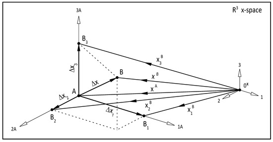
where ${\mathit{d}}^k$ is the $k^{th}$ Cartesian unit vector, as shown in Figure 1.

Figure 1. Formulation of a new set of base vectors $\left(n=3\right)$: $x^A$, $x_1^B$, $x_2^B$, $x_3^B$ and interpolation base points $A$, $B_1$, $B_2$ and $B_3$ from new approximate $x^A$ and from new trial increment (iteration stepsize) $▵x=x^B-x^A={\left[\begin{array}{ccc}▵x_1& ▵x_2& ▵x_3\end{array}\right]}^{\mathrm{T}}$.

It follows from this special construction of the initial trials ${\mathit{x}}_k^B$ that $x_{k,i}^B-x_i^A=0$ for $i\ne k$ and $x_{k,i}^B-x_i^A=▵x_i$ for $i=k$ providing that

$$▵\mathit{x}=\left[x_{i,i}^B-x_i^A\right]=\left[▵x_i\right]$$

(33)

is the “initial trial increment vector”. Let

$$▵{\mathit{f}}_k=\left[▵f_{k,j}\right]=\left[f_{k,j}^B-f_j^A\right]$$

(34)

$\left(j=1,\dots ,m\right)$. Any point on the $n$ dimensional interpolation plane $\mathit{y}\left(\mathit{x}\right)$ can be expressed as

$$\left[\begin{array}{c}\mathit{x}\\ \mathit{y}\left(\mathit{x}\right)\end{array}\right]=\left[\begin{array}{c}{\mathit{x}}^A\\ {\mathit{f}}^A\end{array}\right]+\left[\begin{array}{c}▵\mathit{X}\\ ▵\mathit{F}\end{array}\right]{\mathit{q}}^A,$$

(35)

where

$$▵\mathit{X}=\left[{\mathit{x}}_k^B-{\mathit{x}}^A\right]=\left[\begin{array}{ccc}{x}_{1,1}^B-x_1^A& \cdots & x_{n,1}^B-x_1^A\\ ⋮& \ddots & ⋮\\ x_{1,n}^B-x_n^A& \cdots & x_{n,n}^B-x_n^A\end{array}\right]$$

(36)

$$▵\mathit{F}=\left[{\mathit{f}}_k^B-{\mathit{f}}^A\right]=\left[\begin{array}{ccc}{f}_{1,1}^B-f_1^A& \cdots & f_{n,1}^B-f_1^A\\ ⋮& ⋮& ⋮\\ f_{1,m}^B-f_m^A& \cdots & f_{n,m}^B-f_m^A\end{array}\right]$$

(37)

$\left(k=1,\dots ,n\right)$, ${\mathit{q}}^A$ is a vector with $n$ scalar multipliers $q_i^A\left(i=1,\dots ,n\right)$, and as a consequence of Equation (32),

$$▵\mathit{X}=\left[▵{\mathit{x}}_k\right]=\left[\begin{array}{ccc}▵x_1& \cdots & 0\\ ⋮& \ddots & ⋮\\ 0& \cdots & ▵x_n\end{array}\right]=diag\left(▵x_k\right)$$

(38)

is a diagonal matrix that has great computational advantage. It also follows from Definition (34) that

$$▵\mathit{F}=\left[▵{\mathit{f}}_k\right]=\left[\begin{array}{ccc}▵f_{1,1}& \cdots & ▵f_{n,1}\\ ⋮& ⋮& ⋮\\ ▵f_{1,m}& \cdots & ▵f_{n,m}\end{array}\right].$$

(39)

Let ${\mathit{x}}_{p+1}^A$ be the zero of the n-dimensional interpolation plane ${\mathit{y}}_p\left(\mathit{x}\right)$ with interpolation base points $A_p\left(\begin{array}{cc}{\mathit{x}}_p^A& {\mathit{f}}_p^A\end{array}\right)$ and $B_{k,p}\left(\begin{array}{cc}{\mathit{x}}_{k,p}^B& {\mathit{f}}_{k,p}^B\end{array}\right)$ in the $p^{\mathit{th}}$ iteration. Then, it follows from the zero condition that

$${\mathit{y}}_p\left({\mathit{x}}_{p+1}^A\right)=\mathbf{0}$$

(40)

and from the second row of Equation (35) that

$$▵{\mathit{F}}_p{\mathit{q}}_p^A=-{\mathit{f}}_p^A,$$

(41)

and the vector ${\mathit{q}}_p^A$ of multipliers $q_{p,i}^A$ can be expressed as

$${\mathit{q}}_p^A=-▵{\mathit{F}}_p^{+}{\mathit{f}}_p^A=-\left[\sum _{\mathit{j}=1}^m\left({▵F}_{p,i,j}^{+}{f}_{p,j}^A\right)\right],$$

(42)

where ${\left[.\right]}^{+}$ stands for the pseudo-inverse. Let

$$\left[\begin{array}{c}▵{\mathit{x}}_p^A\\ ▵{\mathit{f}}_p^A\end{array}\right]=\left[\begin{array}{c}{\mathit{x}}_{p+1}^A-{\mathit{x}}_p^A\\ {\mathit{f}}_{p+1}^A-{\mathit{f}}_p^A\end{array}\right]$$

(43)

be the iteration stepsize of the Secant method; then, it follows from the first row of Equation (35) and from Equation (42) that

$$▵{\mathit{x}}_p^A=▵{\mathit{X}}_p{\mathit{q}}_p^A=-▵{\mathit{X}}_p▵{\mathit{F}}_p^{+}{\mathit{f}}_p^A,$$

(44)

and from Definition (43), it follows that

$$\left[\begin{array}{c}{\mathit{x}}_{p+1}^A\\ {\mathit{f}}_{p+1}^A\end{array}\right]=\left[\begin{array}{c}{\mathit{x}}_p^A+▵{\mathit{x}}_p^A\\ {\mathit{f}}_p^A+▵{\mathit{f}}_p^A\end{array}\right],$$

(45)

and the new Secant approximate ${\mathit{x}}_{p+1}^A$ can be expressed from Equation (44) as

$${\mathit{x}}_{p+1}^A={\mathit{x}}_p^A+▵{\mathit{x}}_p^A.$$

(46)

A new base point $A_{p+1}\left({\mathit{x}}_{p+1}^A,{\mathit{f}}_{p+1}^A\right)$ can than be determined for the next iteration. In a single-variable case $\left(m=n=k=1\right)$ with interpolation base points $A_p\left(x_p^A,f_p^A\right)$ and $B_p\left(x_p^B,f_p^B\right)$, Equation (42) will have the form

$$q_p^A=-\frac{f_p^A}{f_p^B-f_p^A}=-\frac{f_p^A}{▵f_p},$$

(47)

and the new Secant approximate

$$x_{p+1}^A=x_p^A+▵x_p{q}_p^A=x_p^A-\frac{▵x_p}{▵f_p}{f}_p^A=\frac{x_p^A{f}_p^B-x_p^B{f}_p^A}{f_p^B-f_p^A}$$

(48)

can be determined according to Equation (46). The procedure then continues with new interpolation base points $A_{p+1}\left(x_{p+1}^A,f_{p+1}^A\right)$ and $B_{p+1}\left(x_{p+1}^B,f_{p+1}^B\right)$.

4. T-Secant Method

4.1. Single-Variable Case

The T-Secant method is different from the traditional Secant method in the way that all interpolation base points $A_p$ and $B_{p,k}$$\left(k=1,\dots ,n\right)$ are updated in each iteration, providing $n+1$ new base points $A_{p+\mathit{1}}$ and $B_{p+1,k}$ for the next iteration. The key idea of the method is very simple. The function value ${\mathit{f}}_{p+1}^A$ (that can be determined from the new Secant approximate ${\mathit{x}}_{p+1}^A$) measures the “distance” of the approximate ${\mathit{x}}_{p+1}^A$ from the root ${\mathit{x}}^{*}$ (if ${\mathit{f}}_{p+1}^A=\mathbf{0}$, then the distance is zero and ${\mathit{x}}_{p+1}^A={\mathit{x}}^{*}$). The T-Secant method uses this information to determine another approximate ${\mathit{x}}_{p+1}^B$. In a single-variable case $\left(m=n=k=1\right)$ with interpolation base points $A_p$ and $B_p$, the basic equation

$$▵f_p{q}_p^A=-{\mathit{f}}_p^A$$

(49)

of the Secant method (Equation (41) in multi-variable case) is modified by a factor

$$t_p^f=\frac{f_{p+1}^A}{f_p^A}$$

(50)

that expresses the “improvement rate” of the new approximate $x_{p+1}^A$ to the original approximate $x_p^A$, providing the T-Secant-modified basic equation

$$t_p^f▵f_p{q}_p^B=-f_p^A.$$

(51)

Then, the T-Secant multiplier

$$q_p^B=\frac{q_p^A}{t_p^f}=-\frac{{\left(f_p^A\right)}^2}{f_{p+1}^A▵f_p}$$

(52)

can be determined. The other basic equation

$$▵x_p^A=▵x_p{q}_p^A$$

(53)

of the Secant method (Equation (44) in multi-variable case) with iteration stepsize

$$▵x_p^A=x_{p+1}^A-x_p^A$$

(54)

is also modified in a similar way to that in the case of Equations (49) and (51) by a factor

$$t_p^x=\frac{x_{p+1}^B-x_{p+1}^A}{x_{p+1}^A-x_p^A}=\frac{▵x_{p+1}}{▵x_p^A}$$

(55)

that expresses the “improvement rate” of the new “T-Secant stepsize” $▵x_{p+1}$ to the previous “secant stepsize” $▵x_p^A$, providing a new basic equation

$$▵x_p^A=t_p^x▵x_p{q}_p^B,$$

(56)

from which

$$▵x_p^A=\frac{▵x_{p+1}}{▵x_p^A}▵x_p{q}_p^B$$

(57)

and

$$x_{p+1}^A-x_p^A=-\frac{x_{p+1}^B-x_{p+1}^A}{x_{p+1}^A-x_p^A}\left(x_p^B-x_p^A\right)\frac{{\left(f_p^A\right)}^2}{f_{p+1}^A\left(f_p^B-f_p^A\right)}.$$

(58)

By re-ordering Equation (58), the T-Secant approximate

$$x_{p+1}^B=x_{p+1}^A+\frac{{\left(▵x_p^A\right)}^2}{▵x_p{q}_p^B}=x_{p+1}^A-\frac{{\left(x_{p+1}^A-x_p^A\right)}^2\left(f_p^B-f_p^A\right)f_{p+1}^A}{\left(x_p^B-x_p^A\right){\left(f_p^A\right)}^2}$$

(59)

can be determined, and it is used to update the original interpolation base point $B_p$ to $B_{p+1}$. The new iteration will then continue with new base points $A_{p+\mathit{1}}$ and $B_{p+1}$. Note that it follows from Equations (52), (53), and (59) that

$$▵x_{p+1}=x_{p+1}^B-x_{p+1}^A=\frac{{\left(▵x_p^A\right)}^2}{▵x_p{q}_p^B}=t_p^f\frac{{\left(▵x_p^A\right)}^2}{▵x_p{q}_p^A}=t_p^f▵x_p^A.$$

(60)

4.2. Multi-Variable Case

In the multi-variable case $\left(m\ge n>1\right)$ with $\left(n+1\right)$ interpolation base points $A_p\left(\begin{array}{cc}{x}_p^A& f_p^A\end{array}\right)$ and $B_{p,k}\left(\begin{array}{cc}{x}_{p,k}^B& f_{p,k}^B\end{array}\right)$$\left(k=1,\dots ,n\right)$, the basic equations of the Secant method (Equations (41) and (44)) are modified as

$${\mathit{T}}_p^F▵{\mathit{F}}_p{\mathit{q}}_p^B=-{\mathit{f}}_p^A$$

(61)

and

$$▵{\mathit{x}}_p^A={\mathit{T}}_p^X▵{\mathit{X}}_p{\mathit{q}}_p^B.$$

(62)

Then, a vector-based equation can be formulated, as in case of the traditional Secant method (see Equation (35)), in a the following form:

$$\left[\begin{array}{c}\mathit{x}-▵\mathit{x}\\ \mathit{z}\left(\mathit{x}\right)\end{array}\right]=\left[\begin{array}{c}{\mathit{x}}^A\\ {\mathit{f}}^A\end{array}\right]+\left[\begin{array}{cc}{\mathit{T}}^X& \mathbf{0}\\ \mathbf{0}& {\mathit{T}}^F\end{array}\right]\left[\begin{array}{c}▵\mathit{X}\\ ▵\mathit{F}\end{array}\right]{\mathit{q}}^B,$$

(63)

where $▵\mathit{X}$ and $▵\mathit{F}$ are defined in (36) and (37), $\mathit{z}\left(\mathit{x}\right)$ is a function with zero at ${\mathit{x}}_{p+\mathit{1}}^B$, and the diagonal transformation matrix in the $p^{\mathit{th}}$ iteration is

$${\mathit{T}}_p=\left[\begin{array}{cc}{\mathit{T}}_p^X& \mathbf{0}\\ \mathbf{0}& {\mathit{T}}_p^F\end{array}\right],$$

(64)

with ${\mathit{T}}_p^X$ and ${\mathit{T}}_p^F$ sub-diagonals, where

$${\mathit{T}}_p^X=diag\left(t_{p,i}^X\right)=\mathit{diag}\left(\frac{x_{p+1,i}^B-x_{p+1,i}^A}{x_{p+1,i}^A-x_{p,i}^A}\right)=\mathit{diag}\left(\frac{▵x_{p+1,i}}{▵x_{p,i}^A}\right)$$

(65)

$${\mathit{T}}_p^F=\mathit{diag}\left(t_{p,j}^F\right)=diag\left(\frac{f_{p+1,j}^B-f_{p+1,j}^A}{f_{p+1,j}^A-f_{p,j}^A}\right),$$

(66)

and ${\mathit{T}}_p^F$ is approximated with the assumption $\mathit{f}\left(\mathit{x}\right)\simeq {\mathit{y}}_p\left({\mathit{x}}_{p+1}^A\right)\simeq {\mathit{z}}_p\left({\mathit{x}}_{p+1}^B\right)$ and according to the conditions ${\mathit{y}}_p\left({\mathit{x}}_{p+1}^A\right)=0$ and ${\mathit{z}}_p\left({\mathit{x}}_{p+1}^B\right)=0$ as

$${\mathit{T}}_p^F\simeq \mathrm{diag}\left(\frac{z_{p,j}\left(x_{p+1}^B\right)-f_{p+1,j}^A}{y_{p,j}\left(x_{p+1}^A\right)-f_{p,j}^A}\right)=diag\left(\frac{f_{p+\mathit{1},j}^A}{f_{p,j}^A}\right)$$

(67)

$\left(i=1,\dots ,n\right)$, $\left(j=1,\dots ,m\right)$, where $f_{p,j}^A\ne 0$. The vector of T-Secant multipliers

$${\mathit{q}}_p^B=-▵{\mathit{F}}_p^{+}{\left({\mathit{T}}_p^F\right)}^{-1}{\mathit{f}}_p^A=-\left[\sum _{j=1}^m\left({▵F}_{p,i,j}^{+}\frac{f_{p,j}^A}{t_{p,j}^F}\right)\right]$$

(68)

can be determined from Equation (61), where ${\left[.\right]}^{+}$ stands for the pseudo-inverse ($▵{\mathit{F}}_p^{+}$ has already been calculated when ${\mathit{q}}_p^A$ was determined from Equation (42)). The $i^{\mathit{th}}$ element of the new approximate ${\mathit{x}}_{p+1}^B$ can be expressed from the $i^{\mathit{th}}$ row of Equation (62):

$$▵x_{p,i}^A=\frac{▵x_{p+1,i}}{▵x_{p,i}^A}▵x_{p,i}{q}_{p,i}^B=\frac{x_{p+1,i}^B-x_{p+1,i}^A}{▵x_{p,i}^A}▵x_{p,i}{q}_{p,i}^B,$$

(69)

and the T-Secant approximate ${\mathit{x}}_{p+1}^B$ can be expressed as

$$x_{p+1,i}^B=x_{p+1,i}^A+\frac{{\left(▵x_{p,i}^A\right)}^2}{▵x_{p,i}{q}_{p,i}^B}=x_{p+1,i}^A-\frac{{\left(▵x_{p,i}^A\right)}^2}{{\displaystyle \sum _{j=1}^m}\left(▵x_{p,i}{▵F}_{p,i,j}^{+}\frac{f_{p,j}^A}{t_{p,j}^F}\right)},$$

(70)

where $▵x_{p,i}\ne 0$ and $q_{p,i}^B\ne 0$ $\left(i=1,\dots ,n\right)$. Then, the next iteration continues with the new trial increment vector (iteration stepsize)

$$▵{\mathit{x}}_{p+1}={\mathit{x}}_{p+1}^B-{\mathit{x}}_{p+1}^A$$

(71)

and with $n+1$ new interpolation base points $A_{p+1}\left(\begin{array}{cc}{\mathit{x}}_{p+1}^A& {\mathit{f}}_{p+1}^A\end{array}\right)$$B_{k,p+1}\left(\begin{array}{cc}{\mathit{x}}_{k,p+1}^B& {\mathit{f}}_{k,p+1}^B\end{array}\right)$$\left(k=1,\dots ,n\right)$. Figure 1 shows the formulation of a set of new base vectors ${\mathit{x}}_{k,p+1}^B$ from ${\mathit{x}}_{p+1}^A$ and ${\mathit{x}}_{p+1}^B$ in the $n=3$ case.

Let the ratio ${\mu }_i$ of constants $q_{p,i}^A$ and $q_{p,i}^B$ be introduced as

$${\mu }_i=\frac{q_{p,i}^A}{q_{p,i}^B}.$$

(72)

Then, it follows from Equations (42), (44), (68), (70), and (71) that the $i^{\mathit{th}}$ element of the new trial increment vector is

$$▵x_{p+1,i}=\frac{{\left(▵x_{p,i}^A\right)}^2}{▵x_{p,i}{q}_{p,i}^B}={\mu }_i\frac{{\left(▵x_{p,i}^A\right)}^2}{▵x_{p,i}{q}_{p,i}^A}={\mu }_i▵x_{p,i}^A.$$

(73)

The basic equations in single-variable and multi-variable cases are summarized in Table 1.

Table 1. Summary of the basic equations (single- and multi-variable cases).

	Single-Variable $\left(\mathit{m}=\mathit{n}=1\right)$	Multi-Variable$\left(\mathit{m}\ge \mathit{n}>1\right)$	Equations
1	$x_p^A$	$x_p^A$
2	$x_p^B$	$x_{p,k}^B=x_p^A+▵x_{p,k}{\mathit{d}}^k$	(32)
3	$▵x_p=x_p^B-x_p^A$	$▵x_p=\left[x_{p,k}^B-x_p^A\right]=diag\left(▵x_{p,i}\right)$	(36), (38)
4	$▵f_p=f_p^B-f_p^A$	$▵{\mathit{F}}_p=\left[\begin{array}{ccc}▵f_{p,1,1}& \cdots & ▵f_{p,n,1}\\ ⋮& \ddots & ⋮\\ ▵f_{p,1,m}& \cdots & ▵f_{p,n,m}\end{array}\right]$	(34), (37), (39)
5	$▵f_p{q}_p^A=-f_p^A$	$▵{\mathit{F}}_p{\mathit{q}}_p^A=-{\mathit{f}}_p^A$	(49), (41)
6	$q_p^A=-\frac{f_p^A}{▵f_p}$	${\mathit{q}}_p^A=-▵{\mathit{F}}_p^{+}{\mathit{f}}_p^A$	(47), (42)
7	$x_{p+1}^A=x_p^A+▵x_p{q}_p^A$	$x_{p+1}^A=x_p^A+▵x_p{\mathit{q}}_p^A$	(48), (46)
8	$▵x_p^A=x_{p+1}^A-x_p^A$	$▵x_p^A=x_{p+1}^A-x_p^A$	(54)
9	$t_p^f=\frac{f_{p+1}^A}{f_p^A}$	${\mathit{T}}_p^F=diag\left(\frac{f_{p+1,j}^A}{f_{p,j}^A}\right)$	(50), (67)
10	$t_p^f▵f_p{q}_p^B=-f_p^A$	${\mathit{T}}_p^F▵{\mathit{F}}_p{\mathit{q}}_p^B=-{\mathit{f}}_p^A$	(51), (61)
11	$q_p^B=\frac{q_p^A}{t_p^f}=-\frac{{\left(f_p^A\right)}^2}{f_{p+1}^A▵f_p}$	${\mathit{q}}_p^B=-▵{\mathit{F}}_p^{+}{\left({\mathit{T}}_p^F\right)}^{-1}{\mathit{f}}_p^A$	(52), (68)
12	$t_p^x=\frac{x_{p+1}^B-x_{p+1}^A}{x_{p+1}^A-x_p^A}=\frac{▵x_{p+1}}{▵x_p^A}$	${\mathit{T}}_p^X=\mathit{diag}\left(\frac{▵x_{p+1,i}}{▵x_{p,i}^A}\right)$	(55), (65)
13	$▵x_p^A=t_p^x▵x_p{q}_p^B$	$▵x_p^A={\mathit{T}}_p^X▵x_p{\mathit{q}}_p^B$	(56), (62)
14	$x_{p+1}^B=x_{p+1}^A+\frac{{\left(▵x_p^A\right)}^2}{▵x_p{q}_p^B}$	$x_{p+1,i}^B=x_{p+1,i}^A+\frac{{\left(▵x_{p,\mathrm{i}}^A\right)}^2}{▵x_{p,i}{q}_{p,i}^B}$	(59), (70)
15	$▵x_{p+1}=t_p^f▵x_p^A$	$▵x_{p+1,i}={\mu }_i▵x_{p,i}^A$	(60), (73)

5. Geometry

5.1. Single-Variable Case

The T-Secant procedure has been worked out for solving multi-variable problems. It can also be applied for solving single-variable ones, however. The geometrical representation of the latter gives a good view with which to explain the mechanism of the procedure.

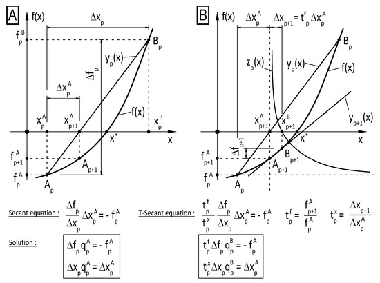
Find the scalar root $x^{*}$ of a nonlinear function $x\to f\left(x\right)$, where $\mathit{x}\in {\mathbb{R}}^1$ and $f:{\mathbb{R}}^1\to {\mathbb{R}}^1$. Let the function $f\left(x\right)$ be linearly interpolated through initial base points $A_p\left(x_p^A,f_p^A\right)$ and $B_p\left(x_p^B,f_p^B\right)$, providing a “secant” line $y_p\left(x\right)$ as shown on Figure 2, where $f_p^A=f\left(x_p^A\right)$ and $f_p^B=f\left(x_p^B\right)$ are the corresponding function values. An arbitrary point of the Secant $y_p\left(x\right)$ can be expressed as

$$\left[\begin{array}{c}x\\ y_p\left(x\right)\end{array}\right]=\left[\begin{array}{c}{x}_p^A\\ f_p^A\end{array}\right]+\left[\begin{array}{c}▵x_p\\ ▵f_p\end{array}\right]q_p^A,$$

(74)

where $q_p^A$ is a scalar multiplier. Let a new approximate $x_{p+1}^A$ be the root of the Secant $y_p\left(x\right)$ and let

$$▵x_p^A=x_{p+1}^A-x_p^A$$

(75)

be the iteration stepsize. It follows from condition

$$y_p\left(x_{p+1}^A\right)=0$$

(76)

and from the second row of Equation (74) that

$$▵f_p{q}_p^A=-f_p^A,$$

(77)

and the scalar multiplier can be determined as

$$q_p^A=-\frac{f_p^A}{▵f_p}.$$

(78)

From the first row of Equation (74), the iteration stepsize is given as

$$▵x_p^A=▵x_p{q}_p^A,$$

(79)

and the new approximate can be expressed as

$$x_{p+1}^A=x_p^A+▵x_p^A.$$

(80)

A new base point $A_{p+1}\left(x_{p+1}^A,f_{p+1}^A\right)$ (see Figure 2) can then be determined for the next iteration. Two out of the three available base points $\left(\begin{array}{ccc}{A}_p& B_p& A_{p+\mathit{1}}\end{array}\right)$ are used for the next iteration by omitting either $A_p$ or $B_p$ in the case of the traditional secant method. The decision is not obvious and it may cause the iteration to unstable and/or not converge to the solution. Instead, an additional new approximate $x_{p+1}^B$ is determined by the T-Secant procedure as a root of the function $z_p\left(x\right)$ near the first Secant approximate $x_{p+1}^A$, and iteration continues with new base points $A_{p+1}\left(x_{p+1}^A,f_{p+1}^A\right)$ and $B_{p+1}\left(x_{p+1}^B,f_{p+1}^B\right)$. An arbitrary point of the function $z_p\left(x\right)$ can be expressed as

$$\left[\begin{array}{c}x-▵x\\ z_p\left(x\right)\end{array}\right]=\left[\begin{array}{c}{x}_p^A\\ f_p^A\end{array}\right]+\left[\begin{array}{cc}{t}^x& 0\\ 0& t^f\end{array}\right]\left[\begin{array}{c}▵x_p\\ ▵f_p\end{array}\right]q_p^B,$$

(81)

where the transformation scalars for $▵x_p$ and $▵f_p$ at $x=x_p^B$ are

$$t_p^x=\frac{▵x_{p+1}}{▵x_p^A}=\frac{x_{p+1}^B-x_{p+1}^A}{x_{p+1}^A-x_p^A}and{t}_p^f=\frac{f_{p+1}^A}{f_p^A}.$$

(82)

Then, it follows from condition

$$z_p\left(x_{p+1}^B\right)=0$$

(83)

and from the second row of Equation (81) that

$$t_p^f▵f_p{q}_p^B=-f_p^A$$

(84)

and

$$q_p^B=-\frac{f_p^A}{t_p^f▵f_p}=-\frac{{\left(f_p^A\right)}^2}{f_{p+1}^A\left(f_p^B-f_p^A\right)}.$$

(85)

The new approximate $x_{p+1}^B$ can then be expressed from the first row of Equation (81) as

$$x_{p+1}^B=x_{p+1}^A+\frac{{\left(▵x_p^A\right)}^2}{▵x_p{q}_p^B}.$$

(86)

The new base point $B_{p+1}\left(x_{p+1}^B,f_{p+1}^B\right)$ (see Figure 2) can then be determined. Interpolation base points $A_{p+1}$ and $B_{p+1}$ are used for the next iteration. The scalar multiplier $q_p^B$ can be expressed from Equation (86) as

$$q_p^B=\frac{{\left(x_{p+1}^A-x_p^A\right)}^2}{\left(x_p^B-x_p^A\right)\left(x_{p+1}^B-x_{p+1}^A\right)}.$$

(87)

By substituting it into the second row of Equation (81) and changing $x_{p+1}^B$ to $x$, it turns into a hyperbolic function

$$z_p\left(x\right)=\frac{a_p}{x-x_{p+1}^A}+f_p^A$$

(88)

with vertical and horizontal asymptotes $x_{p+1}^A$ and $f_p^A$, where

$$a_p={\left(x_{p+1}^A-x_p^A\right)}^2\frac{f_p^B-f_p^A}{x_p^B-x_p^A}\frac{f_{p+1}^A}{f_p^A},$$

(89)

and the root $x_{p+1}^B$ of the function $z_p\left(x\right)$ will be in the vicinity of $x_{p+1}^A$ in “appropriate distance”, which is regulated by the function value $f_{p+1}^A$ (see Figure 2). This virtue of the T-Secant procedure is that it ensures an automatic mechanism for having base vectors in general positions through the whole iteration process, providing a stable and efficient numerical performance.

Figure 2. Geometrical representation of the Secant method in asingle-variable case: (A) classic Secant method; (B) T-Secant modification.

5.2. Multi-Variable Case

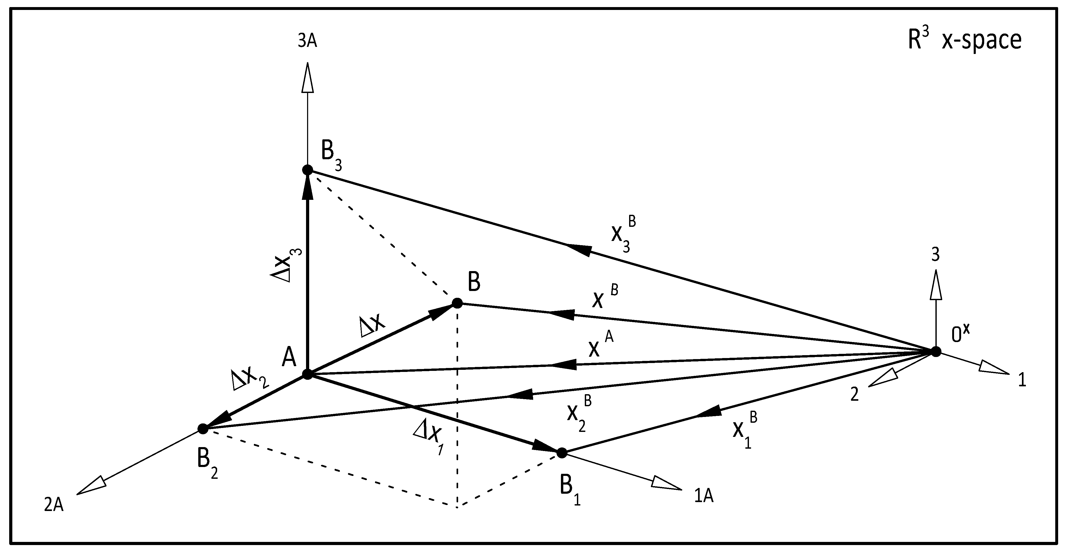
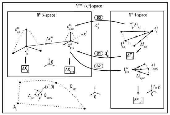
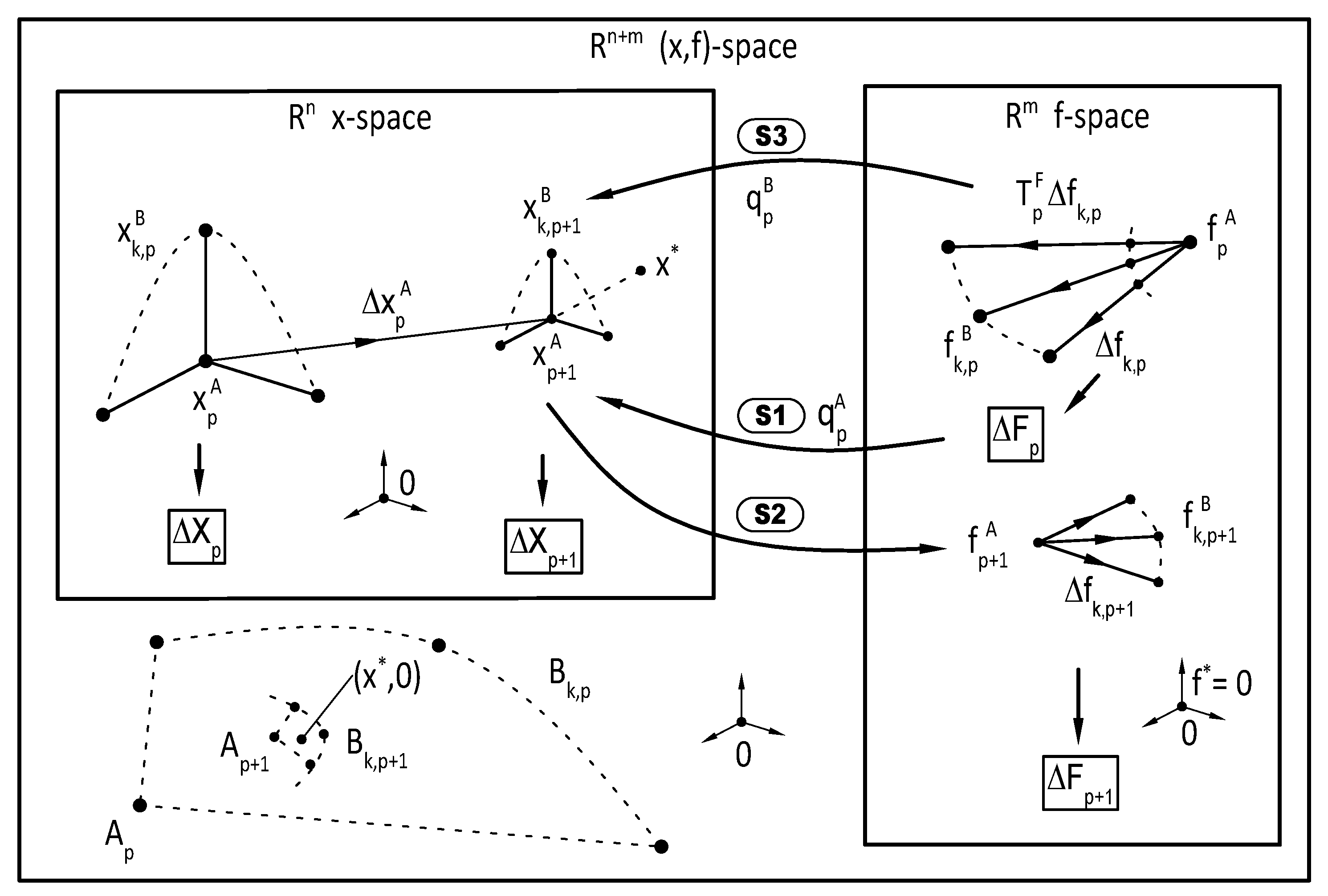
Find the root ${\mathit{x}}^{*}$ of a nonlinear function $\mathit{x}\to \mathit{f}\left(\mathit{x}\right)$, where $\mathit{x}\in {\mathbb{R}}^n$ and $f:{\mathbb{R}}^n\to {\mathbb{R}}^m$. Let the function $\mathit{f}\left(\mathit{x}\right)$ be linearly interpolated through $n+1$ base points $A_p\left({\mathit{x}}_p^A,{\mathit{f}}_p^A\right)$ and $B_{k,p}\left({\mathit{x}}_{k,p}^B,{\mathit{f}}_{k,p}^B\right)$ in the ${\mathit{R}}^{n+m}$ space ($\mathit{f}\left(\mathit{x}\right)-$ space) in the $p^{\mathit{th}}$ iteration as shown on Figure 3, where $\mathit{k}=1,\dots ,n$, given a set of approximates ${\mathit{x}}_p^A$ and

$${\mathit{x}}_{k,p}^B={\mathit{x}}_p^A+▵{\mathit{x}}_{k,p}{\mathit{d}}^k$$

(90)

in the ${\mathbb{R}}^n$ space ($\mathit{x}-$ space) with $k=1,\dots ,n$, where ${\mathit{d}}^k$ is the $k^{th}$ Cartesian unit vector. Let the expression

$$▵{\mathit{F}}_p{\mathit{q}}_p^A=\left[\begin{array}{ccc}▵f_{1,1,p}& \cdots & ▵f_{n,1,p}\\ ⋮& ⋮& ⋮\\ ▵f_{1,m,p}& \cdots & ▵f_{n,m,p}\end{array}\right]{\mathit{q}}_p^A$$

(91)

represent the linear combination ${\mathit{q}}_p^A={\left[q_{p,k}^A\right]}^T$ of $n$ column vectors

$$\left[▵f_{k,j,p}\right]=\left[▵{\mathit{f}}_{k,p}\right]=\left[{\mathit{f}}_{k,p}^B-{\mathit{f}}_{k,p}^A\right]$$

in the ${\mathbb{R}}^m$ space ($\mathit{f}-$ space) with $k=1,\dots ,n$ column index, and with $j=1,\dots ,m$ row index, and the expression

$$▵{\mathit{X}}_p{\mathit{q}}_p^A=\left[\begin{array}{ccc}▵x_{1,1,p}& \cdots & ▵x_{n,1,p}\\ ⋮& ⋮& ⋮\\ ▵x_{1,n,p}& \cdots & ▵x_{n,n,p}\end{array}\right]{\mathit{q}}_p^A$$

(92)

represents the same linear combination of $n$ column vectors

$$\left[▵x_{k,j,p}\right]=\left[▵x_{p,k}\right]=\left[x_{p,k}^B-x_{p,k}^A\right],$$

(93)

with $k=1,\dots ,n$ column index, and with $j=1,\dots ,n$ row index. The linear combination ${\mathit{q}}_p^A$ is determined from Equation (42) in step $S1$ (see Figure 3), providing a new approximate

$${\mathit{x}}_{p+1}^A=\left[x_{p+1,k}^A\right]={\mathit{x}}_p^A+▵{\mathit{x}}_p^A,$$

(94)

for the solution ${\mathit{x}}^{*}$, and the corresponding ${\mathit{f}}_{p+1}^A$ vector is also determined in step $S2$ (see Figure 3). The column vectors $▵{\mathit{f}}_{k,p}$ of $▵{\mathit{F}}_p$ are then modified by a non-uniform scaling transformation,

$${\mathit{T}}_p^F=diag\left(\frac{f_{p+1,j}^A}{f_{p,j}^A}\right),$$

(95)

and a new linear combination ${\mathit{q}}_p^B={\left[q_{p,k}^B\right]}^T$ is determined from Equation (68) in step $S3$ (see Figure 3), providing a new approximate ${\mathit{x}}_{p+1}^B$ for the solution ${\mathit{x}}^{*}$ with elements

$$x_{p+1,k}^B=x_{p+1,k}^A+\frac{{\left(▵x_{p,k}^A\right)}^2}{▵x_{p,k}{q}_{p,k}^B}.$$

(96)

A new set of $n+1$ approximates ${\mathit{x}}_{p+1}^A$ and

$${\mathit{x}}_{k,p+1}^B={\mathit{x}}_{p+1}^A+▵x_{k,p+1}{\mathit{d}}^k$$

(97)

($k=1,\dots ,n$) can then be generated with iteration stepsize

$$▵{\mathit{x}}_{p+1}=\left[▵x_{k,p+1}\right]={\mathit{x}}_{p+1}^B-{\mathit{x}}_{p+1}^A$$

(98)

for the next iteration.

Figure 3. Vector space description of the T-Secant method in the multi-variable case ($k=1,\dots n$).

5.3. Single-Variable Example

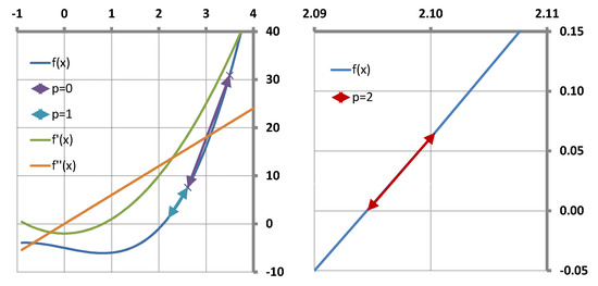
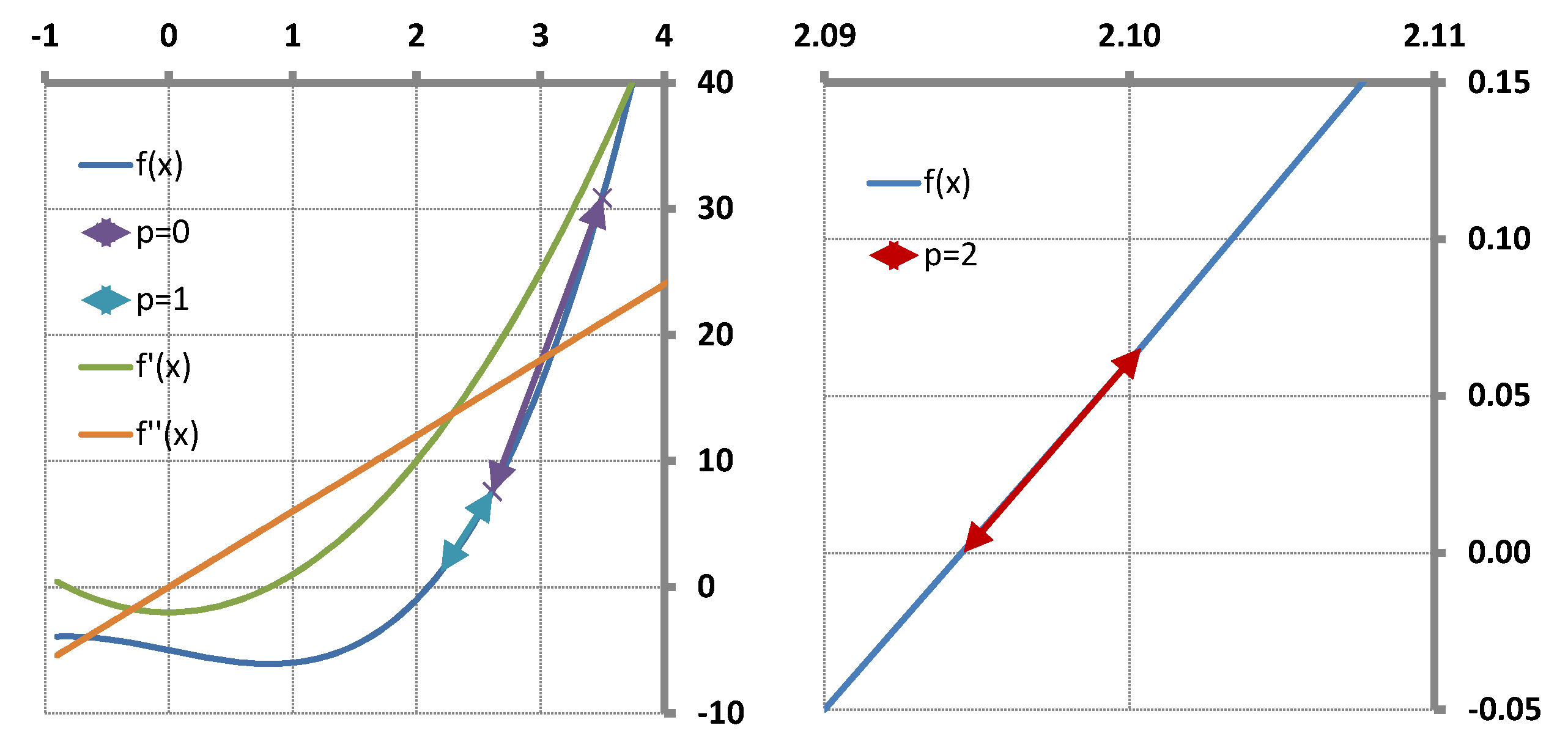
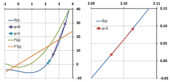
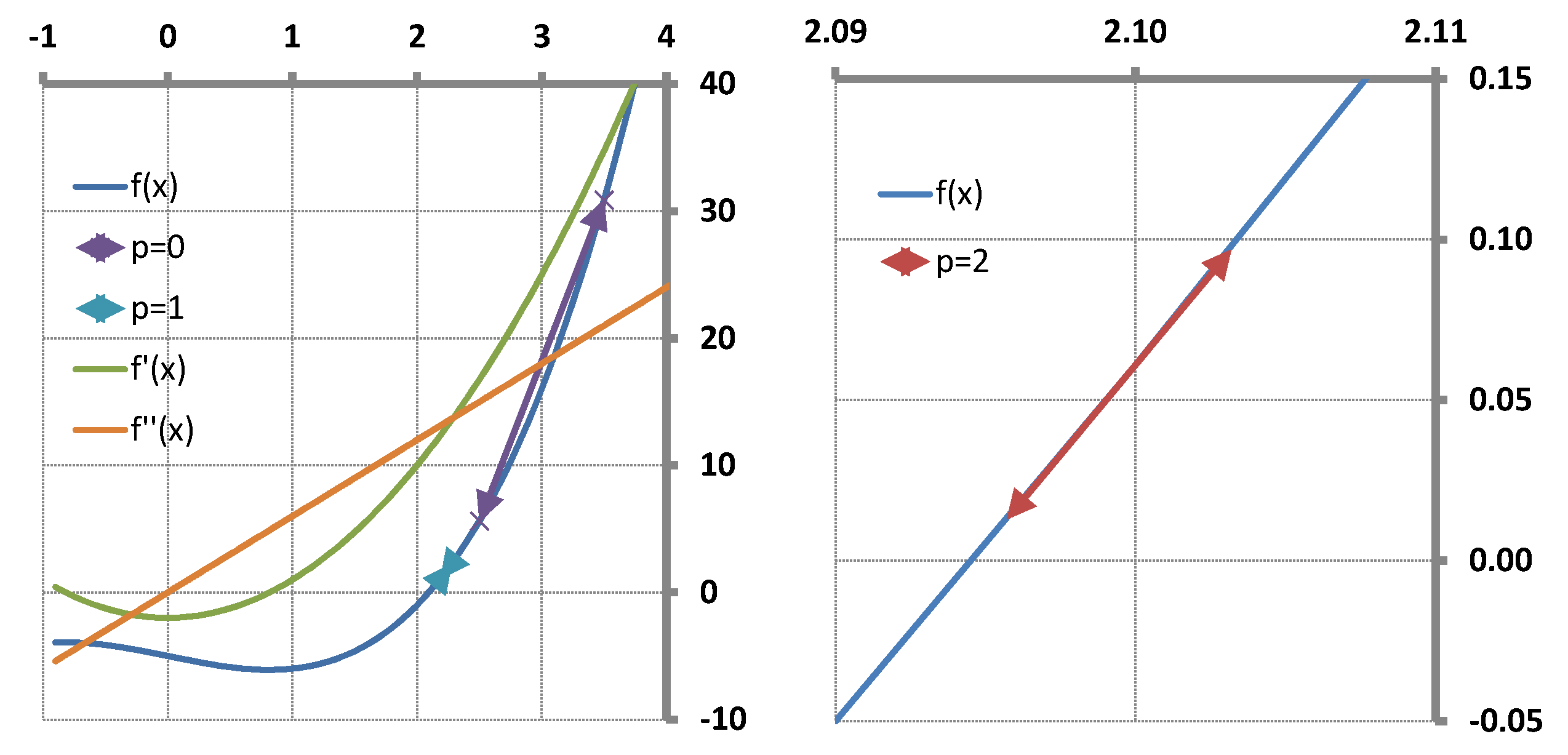
An example is given with function $x\to f\left(x\right)$, where $x\in$ ${\mathbb{R}}^1$$f:{\mathbb{R}}^1\to {\mathbb{R}}^1$ and

$$f\left(x\right)=x^3-2x-5$$

(99)

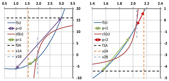
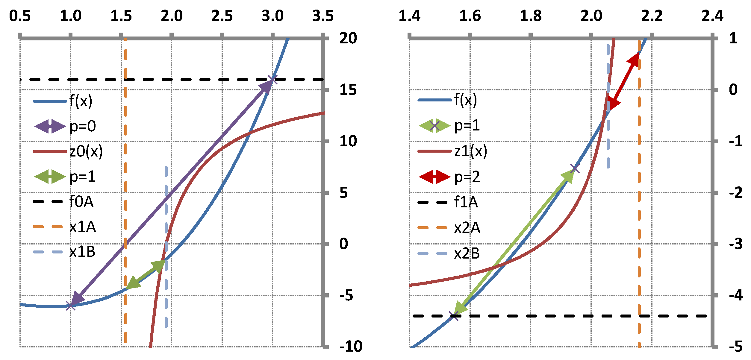
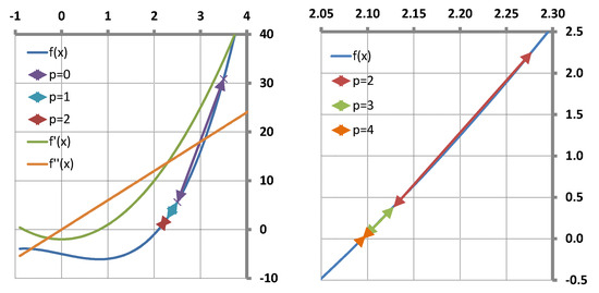
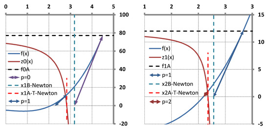
with root $x^{*}\cong 2.0945514815423\dots$. Figure 4 and Table 2 summarize the results of the first two iterations (left: $x_1^A$ is the zero of $y_0\left(x\right)$, $x_1^B$ is the zero of $z_0\left(x\right)$; right: $x_2^A$ is the zero of $y_1\left(x\right)$, $x_2^B$ is the zero of ${\mathit{z}}_1\left(x\right)$). Iterations were made with initial approximates $x_0^A=3.0$ and $x_0^B=1.0$, providing $f_0^A=16$ ($p=0$). The first Secant approximate $x_1^A=1.545\dots$ is found as the zero of the first Secant $y_0\left(x\right)$, and the first T-Secant appropriate $x_1^B=1.945\dots$ is found as the zero of the first hyperbola function $z_0\left(x\right)$ (Figure 4, left). Iteration then goes on ($p=1$) with new interpolation base points $x_1^A=1.545\dots$ and $x_1^B=1.945\dots$ providing $f_1^A=-4.3997\dots$, and new approximates $x_2^A=2.158\dots$ and $x_2^B=2.0556\dots$ are found as the zeros of the second Secant and the second hyperbola function $y_1\left(x\right)$ and $z_1\left(x\right)$, respectively (Figure 4, right). The next iteration ($p=2$) will then continue with interpolation base point $x_2^A=2.158\dots \dots$ and $x_2^B=2.0556\dots$ and with $f_2^A=0.7367\dots$. The iterated values of $f_p^A$$x_p^A$ and $x_p^B$ are also indicated in the diagrams. Further diagrams for this example are shown in Section 7.3.

Figure 4. T-secant iterations with test function (99) with initial approximates $x_0^A=3.0$ and $x_0^B=1.0$ ($\mathbf{Left}$: $x_1^A$ is the root of $y_0\left(x\right)$, $x_1^B$ is the root of $z_0\left(x\right)$; $\mathbf{Right}$: $x_2^A$ is the root of $y_1\left(x\right)$, $x_2^B$ is the root of $z_1\left(x\right)$) (see also Table 2).

Table 2. T-Secant iteration results with $x_0^A=3.0$ and $x_0^B=1.0$ (see also Figure 4 for $p=0,1,2$).

$\mathit{p}$	0	1	2	3	4
$x_p^A$	$3.0$	$1.545$	$2.158$	$2.093$	$2.09455149745$
$▵x_p$	$-2.0$	$0.400$	$-0.103$	$0.0014$	$1.6\times {10}^{-8}$
$f_p^A$	$16.0$	$-4.400$	$0.737$	$-0.015$	$1.8\times {10}^{-7}$
$q_p^A$	$0.727$	$1.532$	$0.634$	$1.015$	$0.999$
$x_{p+1}^A$	$1.545$	$2.158$	$2.093$	$2.09455150$	$2.0945514815423$
$e_{p+1}^A$	$-0.549$	$0.064$	$0.0014$	$1.6\times {10}^{-8}$	$2.7\times {10}^{-14}$
$f_{p+1}^A$	$-4.400$	$0.737$	$-0.015$	$1.8\times {10}^{-7}$
$t_p^F$	$-0.275$	$-0.167$	$-0.021$	$1.2\times {10}^{-5}$
$q_p^B$	$-2.645$	$-9.149$	$-30.329$	$-88077$
$x_{p+1}^B$	$1.945$	$2.056$	$2.09453$	$2.09455148153$

6. General Formulations

Re-ordering Equation (44) gives the general equation

$$▵\mathit{F}▵{\mathit{X}}^{-1}▵{\mathit{x}}^A=-{\mathit{f}}^A$$

(100)

of the Secant method. The initial trials are constructed according to Equation (32), providing that $▵\mathit{X}$ is a diagonal matrix with elements $\left(▵x_i\right)=\left(x_{i,i}^B-x_i^A\right)$ $\left(i=1,\dots ,n\right)$. Let the Jacobean approximate of the secant-method be defined as

$$\mathit{S}=▵\mathit{F}▵{\mathit{X}}^{-1}$$

(101)

$$S=\left[\begin{array}{ccc}\frac{f_{1,1}^B-f_1^A}{x_{1,1}^B-x_1^A}& \cdots & \frac{f_{n,1}^B-f_1^A}{x_{n,1}^B-x_1^A}\\ ⋮& ⋮& ⋮\\ \frac{f_{1,m}^B-f_m^A}{x_{1,1}^B-x_1^A}& \cdots & \frac{f_{n,m}^B-f_m^A}{x_{n,1}^B-x_1^A}\end{array}\right]=\left[\begin{array}{ccc}\frac{▵f_{1,1}}{▵x_1}& \dots & \frac{▵f_{n,1}}{▵x_n}\\ ⋮& ⋮& ⋮\\ \frac{▵f_{1,m}}{▵x_1}& \cdots & \frac{▵f_{n,m}}{▵x_n}\end{array}\right]=\left[\frac{▵f_{k,j}}{▵x_i}\right]$$

(102)

$\left(i=1,\dots ,n\right)$, $\left(j=1,\dots ,m\right)$, $\left(k=1,\dots ,n\right)$ and

$${\mathit{S}}^{+}=▵\mathit{X}▵{\mathit{F}}^{+}.$$

(103)

Then, Equation (100) simplifies as

$$\mathit{S}▵{\mathit{x}}^A=-{\mathit{f}}^A$$

(104)

and

$$▵{\mathit{x}}^A=-{\mathit{S}}^{+}{\mathit{f}}^A.$$

(105)

The $i^{\mathit{th}}$ element of the new approximate ${\mathit{x}}_{p+1}^A$ in the $p^{\mathit{th}}$ iteration will then be

$$x_{p+1,i}^A=x_{p,i}^A+▵x_{p,i}^A=x_{p,i}^A-\sum _{j=1}^m\left(S_{p,i,j}^{+}{f}_{p,j}^A\right)$$

(106)

$\left(i=1,\dots ,n\right)$. It follows from the first row of Equation (63) of the T-Secant method, from Equation (61) and from the Definition (103) of ${\mathit{S}}^{+}$, that the $p^{\mathit{th}}$ iteration stepsize is

$$▵{\mathit{x}}_p^A=-{\mathit{T}}_p^x{\mathit{S}}_p^{+}{\left({\mathit{T}}_p^F\right)}^{-1}{\mathit{f}}_p^A$$

(107)

and

$${\mathit{T}}_p^F{\mathit{S}}_p{\left({\mathit{T}}_p^X\right)}^{-\mathit{1}}▵{\mathit{x}}_p^A=-{\mathit{f}}_p^A.$$

(108)

Let the modified Jacobean approximate of the T-Secant method be defined as

$${\mathit{S}}_{p,T}={\mathit{T}}_p^F{\mathit{S}}_p{\left({\mathit{T}}_p^X\right)}^{-\mathit{1}}$$

(109)

$${\mathit{S}}_{p,T}=\left[\begin{array}{ccc}\frac{f_{p+1,1}^A}{f_{p,1}^A}& 0& 0\\ 0& \ddots & 0\\ 0& 0& \frac{f_{p+1,m}^A}{f_{p,m}^A}\end{array}\right]\left[\begin{array}{ccc}\frac{▵f_{p,1,1}}{▵x_{p,1}}& \dots & \frac{▵f_{p,n,1}}{▵x_{p,n}}\\ ⋮& ⋮& ⋮\\ \frac{▵f_{p,1,m}}{▵x_{p,1}}& \cdots & \frac{▵f_{p,n,m}}{▵x_{p,n}}\end{array}\right]\left[\begin{array}{ccc}\frac{▵x_{p,1}^A}{▵x_{p+1,1}}& 0& 0\\ 0& \ddots & 0\\ 0& 0& \frac{▵x_{p,n}^A}{▵x_{p+1,n}}\end{array}\right]$$

(110)

and in condensed form with general matrix elements (without the $p$ index):

$${\mathit{S}}_T={\mathit{T}}^F\mathit{S}{\left({\mathit{T}}^X\right)}^{-1}=diag\left(t_j^F\right)\left[\frac{▵f_{k,j}}{▵x_i}\right]diag\left(\frac{1}{t_i^X}\right)=\left[\frac{t_j^F}{t_i^X}\frac{▵f_{k,j}}{▵x_i}\right]$$

(111)

$\left(i=1,\dots ,n\right)$, $\left(j=1,\dots ,m\right)$, $\left(k=1,\dots ,n\right)$ and

$${\mathit{S}}_T^{+}={\mathit{T}}^X{\mathit{S}}^{+}{\left({\mathit{T}}^F\right)}^{-1}.$$

(112)

Equations (107) and (108) then can be re-written as

$$▵{\mathit{x}}^A=-{\mathit{S}}_T^{+}{\mathit{f}}^A$$

(113)

and

$${\mathit{S}}_T▵{\mathit{x}}^A=-{\mathit{f}}^A$$

(114)

in a similar form as in case of the traditional Secant method (Equations (105) and (104)). The $i^{\mathit{th}}$ element $x_{p+1,\mathit{i}}^B$ of the second new approximate $x_{p+1}^B$ in the $p^{\mathit{th}}$ iteration will then be

$$x_{p+1,i}^B=x_{p+1,i}^A+▵x_{p+1,i}=x_{p+1,i}^A-\frac{{\left(▵x_{p,i}^A\right)}^2}{{\displaystyle \sum _{j=1}^m}\left(S_{p,i,j}^{+}\frac{f_{p,j}^A}{t_{p,j}^F}\right)},$$

(115)

where $t_{p,j}^F\ne 0$, $\left(j=1,\dots ,m\right)$ and $\left(i=1,\dots ,n\right)$. Note that the T-Secant modification of the Jacobean approximate (102) is made with multipliers

$$t_{p,j}^F=\frac{f_{p+1,j}^A}{f_{p,j}^A}\mathrm{and}{t}_{p,i}^x=\frac{▵x_{p+1,i}}{▵x_{p,i}^A}$$

(116)

to the difference quantities $▵f_{p,k,j}$ and $▵x_{p,i}$. The basic equations of the Secant method and the T-Secant method are summarized in Table 3; rows 1–4 are the elements (matrix $\mathit{T}$) of the basic equations, rows 5–6 are the explicit basic equations, row 7 depicts the Jacobean-type matrices, and rows 8–9 are the general formulations of the basic equations.

Table 3. Summary of the multi-variable Secant and T-Secant methods basic equations.

	Secant Method	T-Secant Method	Equations
1	$\left[\begin{array}{c}▵{\mathit{X}}_p\\ ▵{\mathit{F}}_p\end{array}\right]=\left[\begin{array}{c}{\mathit{x}}_{p,k}^B-{\mathit{x}}_p^A\\ {\mathit{f}}_{p,k}^B-{\mathit{f}}_p^A\end{array}\right]=\left[\begin{array}{c}\mathit{diag}\left(▵x_{p,i}\right)\\ ▵f_{p,k,j}\end{array}\right]$		(36), (37)
2		${\mathit{T}}_p=\left[\begin{array}{cc}{\mathit{T}}_p^X& \mathbf{0}\\ \mathbf{0}& {\mathit{T}}_p^F\end{array}\right]$	(64)
3		${\mathit{T}}_p^X=diag\left(t_{p,i}^x\right)=\mathit{diag}\left(\frac{▵x_{p+1,i}}{▵x_{p,i}^A}\right)$	(65)
4		${\mathit{T}}_p^F=\mathit{diag}\left(t_{p,j}^F\right)\cong diag\left(\frac{f_{p+1,j}^A}{f_{p,j}^A}\right)$	(66), (67)
5	$▵\mathit{F}{\mathit{q}}^A=-{\mathit{f}}^A$	${\mathit{T}}^F▵\mathit{F}{\mathit{q}}^B=-{\mathit{f}}^A$	(41), (61)
6	$▵\mathit{F}▵{\mathit{X}}^{-1}▵{\mathit{x}}^A=-{\mathit{f}}^A$	${\mathit{T}}^F▵\mathit{F}▵{\mathit{X}}^{-1}{\left({\mathit{T}}^X\right)}^{-\mathit{1}}▵{\mathit{x}}^A=-{\mathit{f}}^A$	(100), (108)
7	$\mathit{S}=▵\mathit{F}▵{\mathit{X}}^{-1}=\left[\frac{▵f_{k,j}}{▵x_i}\right]$	${\mathit{S}}_T={\mathit{T}}^F\mathit{S}{\left({\mathit{T}}^X\right)}^{-1}=\left[\frac{t_j^F▵f_{k,j}}{t_i^x▵x_i}\right]$	(102), (111)
8	$\mathit{S}▵{\mathit{x}}^A=-{\mathit{f}}^A$	${\mathit{S}}_T▵{\mathit{x}}^A=-{\mathit{f}}^A$	(104), (114)
9	$▵{\mathit{x}}^A=-{\mathit{S}}^{+}{\mathit{f}}^A$	$▵{\mathit{x}}^A=-{\mathit{S}}_T^{+}{\mathit{f}}^A$	(105), (113)

7. Convergence

7.1. Single-Variable Case

As was shown in Section 4 (Equation (60)), the $p^{\mathit{th}}$ iteration stepsize of the second new approximate $x_{p+1}^B$ is

$$▵x_{p+1}=t_p^f▵x_p^A.$$

(117)

The Secant method is super-linear convergent, so the new approximate $x_{p+1}^A$ is expected to be a much better approximate to the solution $x^{*}$ then the previous one ($x_p^A$). Thus,

$$\left|f_{p+1}^A\right|⋘\left|f_p^A\right|$$

(118)

and

$$\left|t_p^f\right|=\left|\frac{f_{p+1}^A}{f_p^A}\right|⋘1$$

(119)

is expected to be a “small positive number”. It means that the T-Secant approximate $x_{p+1}^B$ will always be in the vicinity of the classic Secant approximate $x_{p+1}^A$, and the approximate errors of the new approximates will be of a similar order, providing that the solution $x^{*}$ will be evenly surrounded by the two new trial approximates $x_{p+1}^A$ and $x_{p+1}^B$.

7.2. Convergence Rate

It is well known that the single-variable Secant method has asymptotic convergence for sufficiently good initial approximates $x^A$ and $x^B$ if $f^{\prime }\left(x\right)$ does not vanish in $x\in \left[\begin{array}{cc}{x}^A& x^B\end{array}\right]$ and $f^{″}\left(x\right)$ is continuous at least in a neighborhood of the zero $x^{*}$. The super-linear convergence property has been proved in different waysm and it is known that the order of convergence ${\alpha }^S=\left(1+\sqrt{5}\right)/2$ with asymptotic error constant

$$C={\left(\frac{1}{2}\left|\frac{f^{″}\left(\xi \right)}{f^{\prime }\left(\xi \right)}\right|\right)}^{\frac{1}{\alpha }}.$$

(120)

The order of convergence of the T-Secant method is determined in this section. Let $p$ be the iteration counter and the approximate error be defined in the $p^{\mathrm{th}}$ iteration as

$$e_p=x_p-x^{*}.$$

(121)

It follows from Equation (48) and from Definition (121) that the error $e_{p+1}^A$ of the new Secant approximate $x_{p+1}^A$ can be expressed as

$$e_{p+1}^A=\frac{e_p^A{f}_p^B-e_p^B{f}_p^A}{f_p^B-f_p^A}=\frac{x_p^B-x_p^A}{f_p^B-f_p^A}\frac{f_p^B/e_p^B-f_p^A/e_p^A}{x_p^B-x_p^A}{e}_p^A{e}_p^B.$$

(122)

It follows from the mean value theorem that the first factor of the right side of Equation (122) can be replaced with $1/f^{\prime }\left({\eta }_p\right)$, where ${\eta }_p\in \left(x_p^A,x_p^B\right)$, if $f\left(x\right)$ is continuously differentiable on $\left(x_p^A,x_p^B\right)$ and $f^{\prime }\left({\eta }_p\right)\ne 0$. Let the function $\mathit{f}\left(x\right)$ be approximated around the root $x^{*}$ by a second order Taylor series expansion as

$$f_p=f\left(e_p+x^{*}\right)=f\left(x^{*}\right)+e_p{f}^{\prime }\left(x^{*}\right)+\frac{1}{2}{\left(e_p\right)}^2{f}^{″}\left({\xi }_p\right),$$

(123)

where ${\xi }_p\in \left(x_p^A,x_p^B,x^{*}\right)$ in the remainder term. Since $f\left(x^{*}\right)=0$, it follows from Equation (123) that

$$\frac{f_p}{e_p}=f^{\prime }\left(x^{*}\right)+\frac{1}{2}{f}^{″}\left({\xi }_p\right)e_p.$$

(124)

Substituting this expression to Equation (122), and since $e_p^B-e_p^A=x_p^B-x_p^A$, we obtain

$$e_{p+1}^A=\frac{1}{2}\frac{f^{″}\left({\xi }_p\right)}{f^{\prime }\left({\eta }_p\right)}\frac{e_p^B-e_p^A}{x_p^B-x_p^A}{e}_p^A{e}_p^B=C_p{e}_p^A{e}_p^B$$

(125)

and

$$C_p=\frac{1}{2}\frac{f^{\prime \prime }\left({\xi }_p\right)}{{\mathit{f}}^{\prime }\left({\eta }_p\right)}.$$

(126)

If the series $\left\{x_p^A\right\}$ converges to $x^{*}$, then ${\xi }_p$ and ${\eta }_p$$\to x^{*}$ with increasing iteration counter $p$, and

$$C_p\to \frac{1}{2}\frac{f^{″}\left(x^{*}\right)}{f^{\prime }\left(x^{*}\right)}=constant.$$

(127)

It follows from Equation (59) with Definition (121) and from the mean value theorem (with ${\eta }_{p-1}\in \left(x_{p-1}^A,x_{p-1}^B\right)$, if $\mathit{f}\left(x\right)$ is continuously differentiable on $\left(x_{p-1}^A,x_{p-1}^B\right)$), that

$$x_p^B=x_p^A-{\left(\frac{x_p^A-x_{p-1}^A}{f_{p-1}^A}\right)}^2{f}^{\prime }\left({\eta }_{p-1}\right)f_p^A,$$

(128)

and the error $e_p^B$ of the T-Secant approximate $x_p^B$ can be expressed as

$$e_p^B=e_p^A-{\left(\frac{e_p^A-e_{p-1}^A}{f_{p-1}^A}\right)}^2{f}^{\prime }\left({\eta }_{p-1}\right)f_p^A.$$

(129)

With the Taylor-series expansion (123) for $f_{p-1}^A$ and $f_p^A$, where ${\xi }_{p-1}\in \left(x_{p-1}^A,x_{p-1}^B,x^{*}\right)$ and ${\xi }_p\in \left(x_p^A,x_p^B,x^{*}\right)$ in the remainder term, we obtain

$$e_p^B=e_p^A-e_p^A{\left(\frac{e_p^A-e_{p-1}^A}{e_{p-1}^A}\right)}^2{\gamma }_p,$$

(130)

where

$${\gamma }_p=\frac{\frac{f^{\prime }\left(x^{*}\right)}{f^{\prime }\left({\eta }_{p-1}\right)}+\frac{1}{2}\frac{f^{″}\left({\xi }_p\right)}{f^{\prime }\left({\eta }_{p-1}\right)}{e}_p^A}{{\left(\frac{f^{\prime }\left(x^{*}\right)}{f^{\prime }\left({\eta }_{p-1}\right)}+\frac{1}{2}\frac{f^{″}\left({\xi }_{p-1}\right)}{f^{\prime }\left({\eta }_{p-1}\right)}{e}_{p-1}^A\right)}^2}$$

(131)

and $f^{\prime }\left({\eta }_{p-1}\right)\ne 0$. If the series $\left\{x_p^A\right\}$ converges to $x^{*}$, then, with increasing iteration counter $p$, ${\xi }_p$, ${\xi }_{p-1}$, ${\eta }_{p-1}$$\to x^{*}$, and $e_p^A$, $e_{p-1}^A\to 0$, it implies that

$$\frac{f^{\prime }\left(x^{*}\right)}{f^{\prime }\left({\eta }_{p-1}\right)}\to \frac{f^{\prime }\left(x^{*}\right)}{f^{\prime }\left(x^{*}\right)}=1$$

(132)

and ${\gamma }_p\to 1$. Substituting $e_p^B$ (Equation (130)) into Equation (125) gives

$$e_{p+1}^A=C_p{e}_p^A\left(e_p^A-e_p^A{\left(\frac{e_p^A-e_{p-1}^A}{e_{p-1}^A}\right)}^2{\gamma }_p\right),$$

(133)

and re-arranging

$$e_{p+1}^A=C_p{e}_p^A\left({\gamma }_p{\left(e_p^A\right)}^2\frac{2e_{p-1}^A-e_p^A}{{\left(e_{p-1}^A\right)}^2}+\left(1-{\gamma }_p\right)e_p^A\right)$$

(134)

with $\left\{x_p^A\right\}$ converges to $x^{*}$, ${\gamma }_p\to 1$, and the above equation simplifies as

$$e_{p+1}^A=C_p{e}_p^A{\left(e_p^A\right)}^2\frac{2e_{p-1}^A-e_p^A}{{\left(e_{p-1}^A\right)}^2}.$$

(135)

This means that $e_{p+1}^A$ depends on $e_p^A$ and $e_{p-1}^A$, and by assuming an asymptotic convergence, a power law relationship

$$\left|e_{p+1}^A\right|=C{\left|e_p^A\right|}^{\alpha }$$

(136)

can be established, where $C$ is the asymptotic error constant and $\alpha$ is the convergence rate, also called the “convergence order” of the iterative method. It also follows from Equation (136), that

$$\left|e_p^A\right|=C{\left|e_{p-1}^A\right|}^{\alpha }$$

(137)

and

$$\left|e_{p-1}^A\right|={\left(\frac{\left|e_p^A\right|}{C}\right)}^{\frac{1}{\alpha }}.$$

(138)

Let $E=\left|e_p^A\right|$ be introduced for simplifying purposes; then, it follows from Equations (133), (136)–(138) that

$$E^{\alpha }=\frac{C_p}{C}{E}^3\frac{2{\left(\frac{E}{C}\right)}^{\frac{1}{\alpha }}-E}{{\left(\frac{E}{C}\right)}^{\frac{2}{\alpha }}},$$

(139)

where $C_p$ and $C$ are constants and, if the series $\left\{x_p^A\right\}$ converges to $x^{*}$, with increasing iteration, counter $p$, $E\to 0^{+}$. Taking the logarithms of both sides of Equation (139) and dividing by $\mathit{lnE}$ gives

$$\alpha =\frac{ln\frac{C_p}{C}}{lnE}+3-\frac{2}{\alpha }·\frac{ln\left(\frac{E}{C}\right)}{lnE}+\frac{ln(2{\left(\frac{E}{C}\right)}^{\frac{1}{\alpha }}-E)}{lnE}.$$

(140)

If $\left\{x_p^A\right\}$ series converges to $x^{*}$, then, with increasing iteration, they counter $p$, $E\to 0^{+}$, $\ln E\to -\infty$ and

$$\underset{E\to 0^{+}}{lim}\frac{ln\frac{C_p}{C}}{lnE}=0$$

(141)

$$\underset{E\to 0^{+}}{lim}ln\left(\frac{E}{C}\right)=\underset{E\to 0^{+}}{lim}\left(lnE-lnC\right)=lnE$$

(142)

$$\underset{E\to 0^{+}}{lim}\frac{ln\left(2E^{\frac{1}{\alpha }}-E\right)}{lnE}=\frac{1}{\alpha },$$

(143)

and Equation (140) simplifies as

$$\alpha -3+\frac{1}{\alpha }=0,$$

(144)

with root (convergence rate of the T-Secant method):

$${\alpha }^{TS}=\frac{3+\sqrt{5}}{2}\cong 2.618033988\dots ={\alpha }^S+1={\phi }^2,$$

(145)

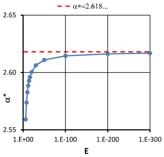
where ${\alpha }^S=\phi \cong 1.618033988\dots$ is the convergence rate of the traditional Secant method, and $\phi$ is the well-known golden ratio. It follows from Equation (140) that the actual values of ${\alpha }^{*}$ of ${\alpha }^{TS}$ depend on the approximate error $E=\left|e^A\right|$. Convergence rates ${\alpha }^{*}\left(E\right)$ were determined for different $E$ values and are shown in Figure 5. The upper bound ${\alpha }^{TS}={\alpha }^S+1=2.618\dots$ at $E\to 0^{+}$ is also indicated (horizontal dashed red line).

Figure 5. ${\alpha }^{*}$ convergence rate variation with decreasing $E\to 0^{+}$ (dashed red lines indicate $\alpha ={\alpha }^S+1\cong 2.618$ level, where ${\alpha }^S\cong 1.618$ is the convergence rate of the traditional Secant method).

7.3. Single-Variable Example

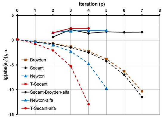
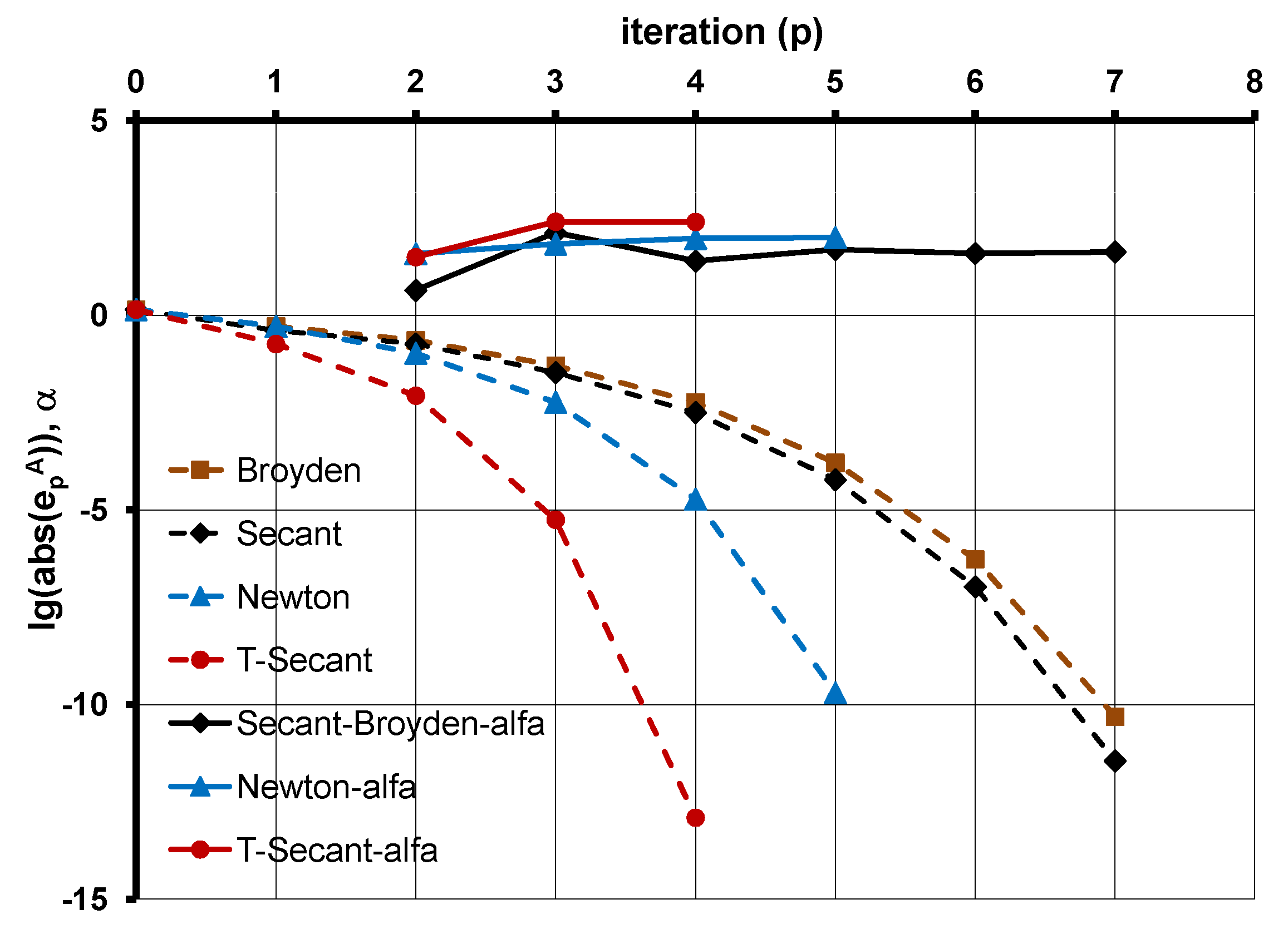
An example is given for demonstration purposes with a single-variable test function (99) with root $x^{*}\cong 2.09455\dots$. Iterations were made with initial approximates $x_0^A=3.5$ and $x_0^B=2.5$, and the convergence rates ${\alpha }^S$, ${\alpha }^N$, and ${\alpha }^{TS}$ were determined for the traditional Secant method (Table 4, Figure 6), for the Newton–Raphson method (Table 5, Figure 7), and for the T-Secant method (Table 6, Figure 8), respectively. The cumulative number of function values ($N_f$) and derivative function values ($N_{f^{\prime }}$) calculations are also indicated in the tables. Calculated convergence rates agree well with theoretical values ${\alpha }^S=1.62\dots$, ${\alpha }^N=2.0$ and ${\alpha }^{TS}=2.62\dots$. Figure 9 summarizes the results of iterations with three different methods (Secant, Newton–Raphson, and T-Secant). Two groups of graphs show the absolute approximate error $\left|e_p^A\right|$ decrease and the calculated convergence rates $\alpha$ for the three compared methods. Results demonstrate that the convergence rate of the T-Secant method is higher than the convergence rate of the Newton–Raphson method.

Table 4. Secant method iteration and computed convergence rate, ${\alpha }^S$ (see Figure 6).

$\mathit{p}$	${\mathit{x}}_{\mathit{p}}^{\mathit{A}}$	${\mathit{x}}_{\mathit{p}}^{\mathit{B}}$	${\mathit{x}}_{\mathit{p}\mathit{+}1}^{\mathit{A}}$	$\left|{\mathit{e}}_{\mathit{p}+1}^{\mathit{A}}\right|$	${\mathit{\alpha }}^{\mathit{S}}$	${\mathit{N}}_{\mathit{f}}$
0	3.5	2.5	2.2772	$1.8\times {10}^{-1}$		2
1	2.5	2.2772	2.1282	$3.4\times {10}^{-2}$		3
2	2.2772	2.1282	2.0977	$3.2\times {10}^{-3}$	0.64	4
3	2.1282	2.0977	2.094611	$5.9\times {10}^{-5}$	2.12	5
4	2.0977	2.094611	2.094552	$1.1\times {10}^{-7}$	1.39	6
5	2.094611	2.09455216	2.09455148	$3.6\times {10}^{-12}$	1.69	7
6	2.0945516	2.09455148	2.09455148154233	$2.7\times {10}^{-14}$	1.59	8
7	2.09455148	2.09455148154233	2.09455148154233	$2.7\times {10}^{-14}$	1.63	9

Figure 6. Secant iteration with test function (99) with initial approximates $x_0^A=3.5$ and $x_0^B=2.5$ ($\mathbf{Left}$: $p=0,1,$2; $\mathbf{Right}$: $p=2,3,4$ (see data in Table 4)).

Table 5. Newton method iteration and computed convergence rate, ${\alpha }^N$ (see Figure 7).

$\mathit{p}$	${\mathit{x}}_{\mathit{p}}^{\mathit{A}}$	${\mathit{x}}_{\mathit{p}+1}^{\mathit{A}}$	$\left|{\mathit{e}}_{\mathit{p}+1}^{\mathit{A}}\right|$	${\mathit{\alpha }}^{\mathit{N}}$	${\mathit{N}}_{\mathit{f}}$	${\mathit{N}}_{{\mathit{f}}^{\prime }}$
0	3.5	2.61	$5.2\times {10}^{-1}$		1	1
1	2.61	2.200	$1.1\times {10}^{-1}$		2	2
2	2.200	2.10037	$5.8\times {10}^{-3}$	1.58	3	3
3	2.10037	2.09457	$1.9\times {10}^{-5}$	1.82	4	4
4	2.09457	2.09455148	$2.0\times {10}^{-10}$	1.97	5	5
5	2.09455148	2.09455148154233	$2.7\times {10}^{-14}$	2.00	6	6

Figure 7. Newton iteration with test function (99) with initial approximate $x_0^A=3.5$ ($\mathbf{Left}$: $p=0,1$; $\mathbf{Right}$: $p=2$ (see data in Table 5)).

Table 6. T-Secant method iteration and computed convergence rate, ${\alpha }^{TS}$ (see Figure 8).

$\mathit{p}$	${\mathit{x}}_{\mathit{p}}^{\mathit{A}}$	${\mathit{x}}_{\mathit{p}}^{\mathit{B}}$	${\mathit{x}}_{\mathit{p}+1}^{\mathit{A}}$	$\left|{\mathit{e}}_{\mathit{p}+1}^{\mathit{A}}\right|$	${\mathit{\alpha }}^{\mathit{TS}}$	${\mathit{N}}_{\mathit{f}}$
0	3.5	2.5	2.28	$1.8\times {10}^{-1}$		2
1	2.28	2.1879	2.1032	$8.6\times {10}^{-3}$		4
2	2.1032	2.0957112	2.0945571	$5.6\times {10}^{-6}$	1.50	6
3	2.0945571	2.09455151	2.09455148154242	$1.2\times {10}^{-13}$	2.41	8
4	2.09455148154242	2.09455148154233	2.09455148154233	$2.7\times {10}^{-14}$	2.40	10

Figure 8. T-Secant iteration with test function (99) with initial approximates $x_0^A=3.5$ and $x_0^B=2.5$ ($\mathbf{Left}$: $p=0$ (with interpolation base points $A_0$$B_0$) and $p=1$ ($A_1$$B_1$); $\mathbf{Right}$: $p=2$ ($A_2$$B_2$) (see data in Table 6)).

Figure 9. Absolute approximate error $\left|e_p^A\right|$ decrease (dashed lines) and computed convergence rates ($\alpha$) (solid lines) of different methods (Broyden (brown line), Secant (black lines), Newton–Raphson (blue lines), and T-Secant (red lines) method).

7.4. Multi-Variable Convergence

Matrix $\mathit{S}$ (see Equation (102)) corresponds to a divided difference approximation of the Jacobian. It is known (e.g., from Dennis-Schnabel [13]) that these values give a second-order approximation of the derivative in the midpoint. When considering Newton’s iteration, it is assumed that the Jacobian has inverted in a neighborhood of ${\mathit{x}}^{*}$. If that condition holds, then there is a chance that the approximate Jacobian has also inverted in the same neighborhood.

It is known that the Secant method is locally q-super-linear convergent, so the new approximate ${\mathit{x}}_{p+1}^A$ is expected to be a much better approximate to the solution ${\mathit{x}}^{*}$ then the previous approximate ${\mathit{x}}_p^A$. Thus,

$$∥{\mathit{f}}_{p+1}^A∥⋘∥{\mathit{f}}_p^A∥$$

(146)

and the diagonal elements

$$\left|t_{p,j}^F\right|=\left|\frac{f_{p+1,j}^A}{f_{p,j}^A}\right|⋘1$$

(147)

of the transformation matrix ${\mathit{T}}_p^F$$\left(j=1\dots ,m\right)$ are expected to be “small numbers”. It follows from Equations (68), (70), (73), and (147) that

$${\mu }_i=\frac{{\displaystyle \sum _{j=1}^m}\left(S_{p,i,j}^{+}{f}_{p,j}^A\right)}{{\displaystyle \sum _{j=1}^m}\left(S_{p,i,j}^{+}\frac{f_{p,j}^A}{t_{p,j}^F}\right)}⋘1$$

(148)

$\left(i=1\dots ,n\right)$ and

$$∥▵{\mathit{x}}_{p+1}∥\le ∥\mathit{\mu }∥∥▵{\mathit{x}}_p^A∥⋘∥▵{\mathit{x}}_p^A∥$$

(149)

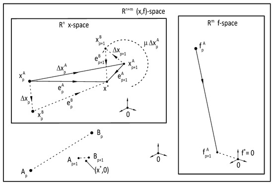
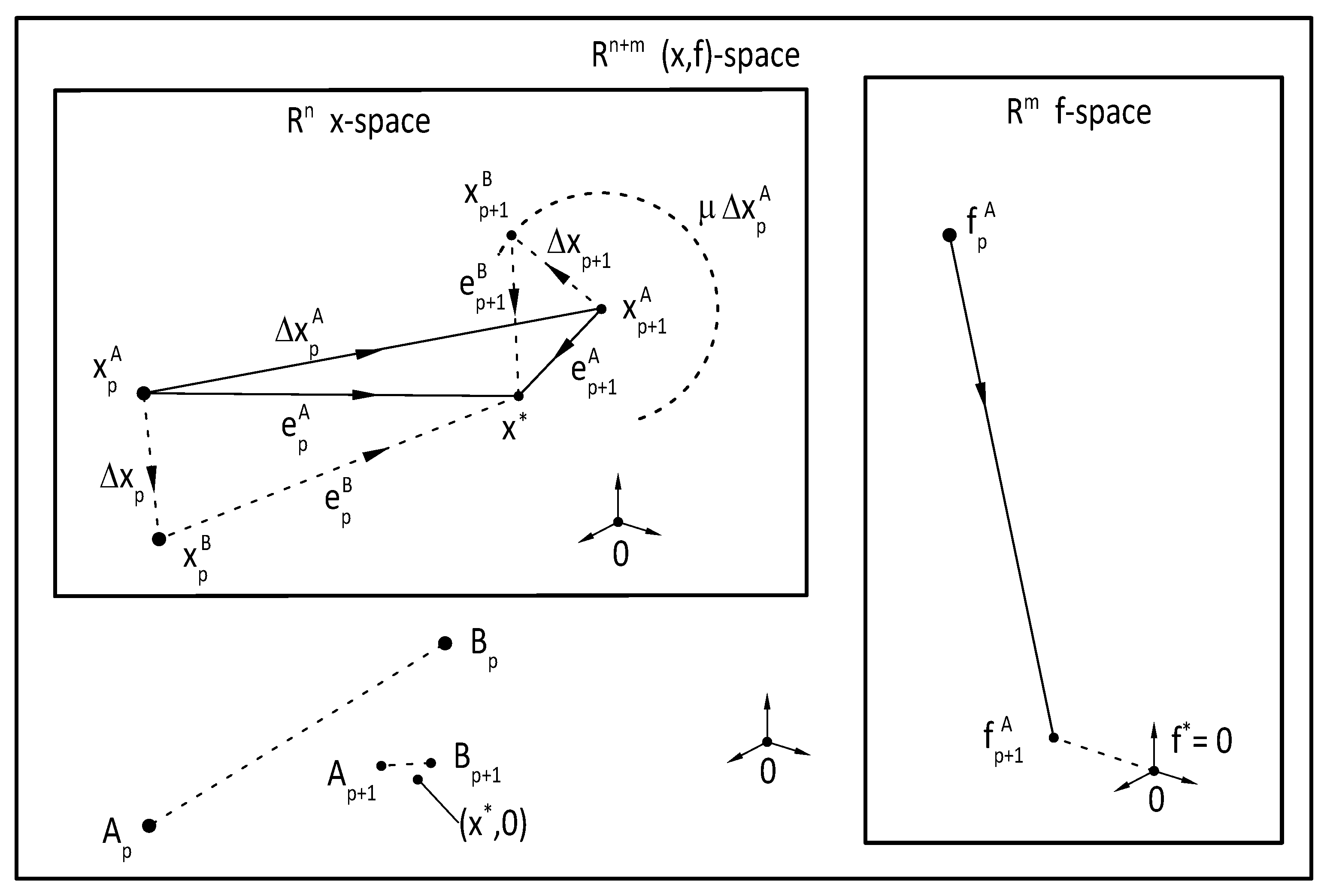
(see Figure 10). This means that the T-Secant approximate ${\mathit{x}}_{p+1}^B$ will always be in the vicinity of the classic Secant approximate ${\mathit{x}}_{p+1}^A$ and the approximate errors of the new approximates will be of similar order, providing that the solution ${\mathit{x}}^{*}$ will be evenly surrounded by the $n+1$ new trial approximates ${\mathit{x}}_{p+1}^A$ and ${\mathit{x}}_{k,p+1}^B$ $\left(k=1\dots ,n\right)$, and that matrix ${\mathit{S}}_{p+1}$ will be well-conditioned.

Figure 10. Geometrical representation of the T-Secant method convergence in multi-variable case (analogous to the convergence proof figure Dennis-Schnabel [13], p. 180).

8. Algorithm

Let $p$ be the iteration counter, ${\epsilon }^{*}$ be the error bound for termination criterion, and

$${\mathit{e}}_p^A={\mathit{x}}_p^A-{\mathit{x}}^{*}$$

(150)

be the approximate error vector of approximate $x^A$ in the $p^{\mathit{th}}$ iteration with elements $e_{p,i}^A$ $\left(i=1,\dots ,n\right)$. Let the scalar approximate error

$${\epsilon }_p=\frac{{∥{\mathit{e}}_p^A∥}_2}{n}=\frac{\sqrt{{\displaystyle \sum _{\mathit{i}=\mathit{1}}^{\mathit{n}}}{\left(e_{p,i}^A\right)}^2}}{n}$$

(151)

be defined, where ${∥.∥}_2$ is the Euclidean norm, and let the iteration be terminated when

$${\epsilon }_p<{\epsilon }^{*}$$

(152)

holds. Let ${\mathit{x}}_p^A$ be the initial trial and $▵{\mathit{x}}_p$ be the trial increment (iteration stepsize) in the $p^{th}$ iteration. Choose $T_{\mathit{min}}$ and $T_{\mathit{max}}$ as lower and upper bounds for $\left|t_{p,j}^F\right|$ $\left(j=1\dots ,m\right)$ and let $f_{\mathit{min}}$ and $q_{\mathit{min}}$ be lower bounds for $\left|f_{p,j}^A\right|$ $\left(j=1,\dots ,m\right)$ and $\left|q_{p,i}^B\right|$$\left(i=1,\dots ,n\right)$, respectively.

• Initial step
  Let $p=0$ and let the initial trial ${\mathit{x}}_p^A=\left(\begin{array}{ccc}{x}_{p,1}^A& \cdots & x_{p,\mathrm{n}}^A\end{array}\right)$ and the initial trial increment $▵{\mathit{x}}_p=\left(\begin{array}{ccc}▵x_{p,1}& \cdots & ▵x_{p,\mathrm{n}}\end{array}\right)$ be given. Calculate the corresponding function values ${\mathit{f}}_p^A$ and assume that $f_{\mathit{min}}<\left|f_{p,j}^A\right|(j=1\dots ,m)$.
• Step 1: Generate a set of $\mathrm{n}$ additional initial trials (interpolation base points)

  $${\mathit{x}}_{p,k}^B={\mathit{x}}_p^A+▵x_{p,k}·{\mathit{d}}^k$$

  (153)

  and evaluate function values ${\mathit{f}}_{p,k}^B$ $\left(k=1,\dots ,n\right)$.
• Step 2 (Secant): Construct matrix

  $$▵{\mathit{F}}_p=\left[▵{\mathit{f}}_{p,k}^i\right]=\left[{\mathit{f}}_{p,k}^B-{\mathit{f}}_p^A\right]$$

  (154)

  then calculate ${\mathit{q}}_p^A$ from Equation (42). Let $q_{\mathit{min}}<\left|q_{p,i}^A\right|$, and determine ${\mathit{x}}_{p+1}^A$ from Equation (46) and ${\epsilon }_p$ from Equation (151).
• Step 3: If ${\epsilon }_p$<${\epsilon }^{*}$, then terminate iteration; otherwise, continue with Step 4.
• Step 4 (T-Secant): Calculate ${\mathit{f}}_{p+1}^A$ and ${\mathit{T}}_p^F$ from Equation (67). Let $T_{\mathit{min}}<\left|t_{p,j}^F\right|<T_{\mathit{max}}$ and determine ${\mathit{q}}_p^B$ from Equation (68) ($▵{\mathit{F}}_p^{+}$ has already been calculated when ${\mathit{q}}_p^A$ was determined from Equation (42)). Let $q_{\mathit{min}}<\left|q_{p,i}^B\right|$. Calculate ${\mathit{x}}_{p+1}^B$ from Equation (70).
• Step 5: Let the new initial trial be

  $$\left[\begin{array}{c}{\mathit{x}}_{p+1}^A\\ {\mathit{f}}_{p+1}^A\end{array}\right]$$

  (155)

  and the new initial trial increment (iteration stepsize) be

  $$▵{\mathit{x}}_{p+1}={\mathit{x}}_{p+1}^B-{\mathit{x}}_{p+1}^A,$$

  (156)

  and continue iteration with Step 1.

Iteration constants $\left(\begin{array}{ccccc}{\delta }_{min}& f_{min}& q_{min}& T_{min}& T_{max}\end{array}\right)$ are necessary in order to avoid division by zero and to avoid computed values being near numerical precision. If $p_{\mathit{max}}$ is the number of necessary iterations for satisfying the termination criterion ${\epsilon }_p<{\epsilon }^{*}$, and $n$ is the number of unknowns to be determined, then the T-Secant method needs $n+1$ function evaluations in each iteration, as well as

$$N_f=p_{\mathit{max}}\left(n+1\right)$$

(157)

function evaluations to reach the desired termination criterion. $p_{\mathit{max}}$ depends on many circumstances, such as the nature of the function $f\left(x\right)$, termination criteria (${\epsilon }^{*}$ or others), and the distance of the initial trial ${\mathit{x}}^A$ from the solution ${\mathit{x}}^{*}$ and from the iteration constants $\left(T_{\mathit{min}},q_{\mathit{min}}^A,\dots \right)$.

9. Numerical Tests Results

9.1. Rosenbrock Test Function

A variant of the Rosenbrock function [24] has been used to test the numerical performance of the suggested method. The global minimum of the function

$$R\left(x\right)=\sum _{i=1}^{N-1}\left(\mathit{100}·{\left(x_{\mathit{i}+1}-x_i^2\right)}^2+{\left(1-x_{\mathit{i}}\right)}^2\right)$$

(158)

has to be determined, where $\mathit{x}=\left(\begin{array}{ccc}{x}_1& \cdots & x_N\end{array}\right)\in {\mathbb{R}}^N$ and $N\ge 2$. $R\left(\mathit{x}\right)$ has exactly one minimum for $N=3$ at ${\mathit{x}}^{*}=$$\left(\begin{array}{ccc}1& 1& 1\end{array}\right)$ and exactly two minima for $4\le N\le 7$, i.e., a global minimum of all and a local minimum near $\widehat{\mathit{x}}=\left(\begin{array}{cccc}-1& 1& \cdots & 1\end{array}\right)$. The sum of squares $\mathrm{R}\left(\mathit{x}\right)$ will be minimum when all terms are zero, such that the minimization of the function $\mathrm{R}\left(\mathit{x}\right)$ is equivalent to finding the zero of a function $\mathit{x}\to \mathit{f}\left(\mathit{x}\right)$, where $\mathit{x}\in {\mathbb{R}}^{\mathrm{N}}$, $\mathit{f}:{\mathbb{R}}^N\to {\mathbb{R}}^{2(N-1)}$, and

$$\mathit{f}\left(x\right)=\left[\begin{array}{c}{f}_{2\mathrm{i}-1}\left(\mathit{x}\right)\\ f_{2\mathrm{i}}\left(\mathit{x}\right)\end{array}\right]=\left[\begin{array}{c}10·(x_{\mathrm{i}+1}-x_{\mathrm{i}}^2)\\ 1-x_{\mathrm{i}}\end{array}\right]$$

(159)

$\left(i=1,\dots ,N-1\right)$. For $\mathrm{N}>7$, the function $\mathrm{R}\left(\mathit{x}\right)$ has exactly one global minimum and has some local minima with some $x_{\mathrm{j}}^{*}=-1$, with $x_{\mathrm{i}}^{*}=1$ for all other unknowns. The results were obtained by least squares solving of the simultaneous system of nonlinear equations $\mathit{f}\left(\mathit{x}\right)=\mathbf{0}$ via the T-Secant method.

9.2. $N=2$, $N=3$ and $N=10$ Examples

In case the case of $N=n=m=2$, the iterations terminated after $N_f=6$ function evaluations ($p_{\mathit{max}}=2$ iterations) in most cases. $f_2\left(\mathit{x}\right)=1-x_1$ is a linear function, and the first T-Secant iteration $\left(p=0\right)$ finds the exact value of $x_1$ in one step; then, $f_1\left(\mathit{x}\right)=10\left(x_2-x_1^2\right)$ also becomes linear. The exact value of $x_2$ was then determined in one additional step.

Let $N=n=3$ and $m=4$, $T_{\mathit{min}}=0.01$ and ${\epsilon }^{*}={10}^{-14}$. Let $p=0$, and

$$▵x_{0,i}=0.05·x_{0,i}^A$$

(160)

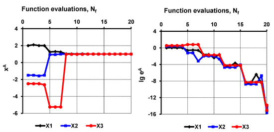
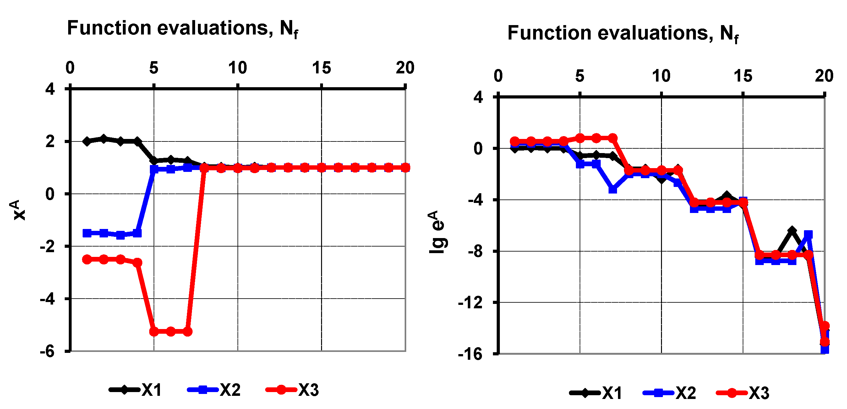
$(\mathrm{i}=1\dots ,3)$. The number of necessary function evaluations $N_f$ varied between 20 and 36 within $p_{\mathit{max}}=5-9$ iterations for different initial trials ${\mathit{x}}_0^A$. Iteration results are summarized in Table 7 and in Figure 11 with initial trial ${\mathit{x}}_0^A=\left({\mathit{x}}_{0,\mathit{i}}^A\right)=\left(\begin{array}{ccc}2.0& -1.5& -2.5\end{array}\right)$. Termination criterion ${\epsilon }_p<{\epsilon }^{*}$ was satisfied after $p_{\mathit{max}}=5$ iterations with $N_f=20$ function evaluations.

Table 7. Iteration results: ${\mathit{x}}_0^A=\left(\begin{array}{ccc}2.0& -1.5& -2.5\end{array}\right)$, $T_{\mathit{min}}=0.01$, $T_{\mathit{max}}=1.5$.

$\mathit{p}$	0	1	2	3
${\mathit{x}}_p^A$	$\left[\begin{array}{c}2\\ -1.5\\ -2.5\end{array}\right]$	$\left[\begin{array}{c}1.253\\ 0.938\\ -5.248\end{array}\right]$	$\left[\begin{array}{c}1.026\\ 0.990\\ 0.980\end{array}\right]$	$\left[\begin{array}{c}1.00004\\ 0.99998\\ 0.99994\end{array}\right]$
$▵{\mathit{x}}_p$	$\left[\begin{array}{c}0.1\\ -0.075\\ -0.125\end{array}\right]$	$\left[\begin{array}{c}0.046\\ 0.061\\ -0.026\end{array}\right]$	$\left[\begin{array}{c}-0.0217\\ 0.0079\\ -0.063\end{array}\right]$	$\left[\begin{array}{c}-3\times {10}^{-4}\\ 1\times {10}^{-4}\\ 2\times {10}^{-4}\end{array}\right]$
${\mathit{f}}_p^A$	$\left[\begin{array}{c}-55\\ -1\\ -47.5\\ 2.5\end{array}\right]$	$\left[\begin{array}{c}-6.320\\ -0.253\\ -61.28\\ 0.062\end{array}\right]$	$\left[\begin{array}{c}-0.621\\ -0.026\\ 0.005\\ 0.010\end{array}\right]$	$\left[\begin{array}{c}-0.00102\\ -0.00004\\ -0.00021\\ 0.00002\end{array}\right]$
${\mathit{q}}_p^A$	$\left[\begin{array}{c}7.47\\ 32.5\\ -22.0\end{array}\right]$	$\left[\begin{array}{c}4.915\\ -0.846\\ 243.9\end{array}\right]$	$\left[\begin{array}{c}-1.184\\ -1.269\\ 0.307\end{array}\right]$	$\left[\begin{array}{c}-0.160\\ -0.201\\ -0.327\end{array}\right]$
${\mathit{x}}_{p+1}^A$	$\left[\begin{array}{c}1.253\\ 0.938\\ -5.248\end{array}\right]$	$\left[\begin{array}{c}1.026\\ 0.990\\ 0.980\end{array}\right]$	$\left[\begin{array}{c}1.00004\\ 0.99998\\ 0.99994\end{array}\right]$	$\left[\begin{array}{c}0.9\dots \\ 1.0\dots \\ 1.0\dots \end{array}\right]$
${\mathit{e}}_{p+1}^A$	$\left[\begin{array}{c}0.253\\ 0.062\\ 6.248\end{array}\right]$	$\left[\begin{array}{c}0.026\\ 0.010\\ 0.020\end{array}\right]$	$\left[\begin{array}{c}4\times {10}^{-5}\\ 2\times {10}^{-5}\\ 6\times {10}^{-5}\end{array}\right]$	$\left[\begin{array}{c}3\times {10}^{-9}\\ 2\times {10}^{-9}\\ 5\times {10}^{-9}\end{array}\right]$
$R\left({\mathit{x}}_{p+1}^A\right)$	$6.2\times {10}^1$	$6.2\times {10}^{-1}$	$1.0\times {10}^{-3}$	$9.0\times {10}^{-8}$
${\epsilon }_p$	$2.1\times {10}^0$	$1.1\times {10}^{-2}$	$2.6\times {10}^{-5}$	$2.2\times {10}^{-9}$
${\mathit{f}}_{p+1}^A$	$\left[\begin{array}{c}-6.32\\ -0.253\\ -61.3\\ 0.062\end{array}\right]$	$\left[\begin{array}{c}-0.621\\ -0.026\\ 0.005\\ 0.010\end{array}\right]$	$\left[\begin{array}{c}-0.00102\\ -0.00004\\ -0.00021\\ 0.00002\end{array}\right]$	$\left[\begin{array}{c}0.0\dots \\ 0.0\dots \\ 0.0\dots \\ -0.0\dots \end{array}\right]$
$t_p^F$	$\left[\begin{array}{c}0.115\\ 0.253\\ 1.290\\ 0.025\end{array}\right]$	$\left[\begin{array}{c}0.098\\ 0.102\\ -0.01\\ 0.163\end{array}\right]$	$\left[\begin{array}{c}0.01\\ 0.01\\ -0.044\\ 0.01\end{array}\right]$	$\left[\begin{array}{c}-0.01\\ -0.01\\ -0.01\\ -0.01\end{array}\right]$
${\mathit{q}}_p^B$	$\left[\begin{array}{c}-120\\ 1298\\ -2365\end{array}\right]$	$\left[\begin{array}{c}51.6\\ -5.52\\ -240000\end{array}\right]$	$\left[\begin{array}{c}-118\\ -127\\ 32\end{array}\right]$	$\left[\begin{array}{c}16.0\\ 20.1\\ 32.7\end{array}\right]$
${\mathit{x}}_{p+1}^B$	$\left[\begin{array}{c}1.299\\ 0.999\\ -5.273\end{array}\right]$	$\left[\begin{array}{c}1.004\\ 0.998\\ 0.917\end{array}\right]$	$\left[\begin{array}{c}0.99978\\ 1.00008\\ 1.00013\end{array}\right]$	$\left[\begin{array}{c}1.0\dots \\ 0.9\dots \\ 0.9\dots \end{array}\right]$
$▵{\mathit{x}}_{p+1}$	$\left[\begin{array}{c}0.046\\ 0.061\\ -0.026\end{array}\right]$	$\left[\begin{array}{c}-0.0217\\ 0.0079\\ -0.063\end{array}\right]$	$\left[\begin{array}{c}-3\times {10}^{-4}\\ 1\times {10}^{-4}\\ 2\times {10}^{-4}\end{array}\right]$	$\left[\begin{array}{c}4\times {10}^{-7}\\ -2\times {10}^{-7}\\ -6\times {10}^{-7}\end{array}\right]$

Figure 11. $\left(\mathbf{Left}\right)$ Variables $x_{p,i}^A$ and $\left(\mathbf{Right}\right)$ absolute approximate errors $\mathit{lg}\left|e_p^A\left(x_{p,i}^A\right)\right|$$\left(i=1\dots 3\right)$ variation for initial trial ${\mathit{x}}_0^A=\left(\begin{array}{ccc}2.0& -1.5& -2.5\end{array}\right)$.

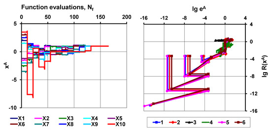
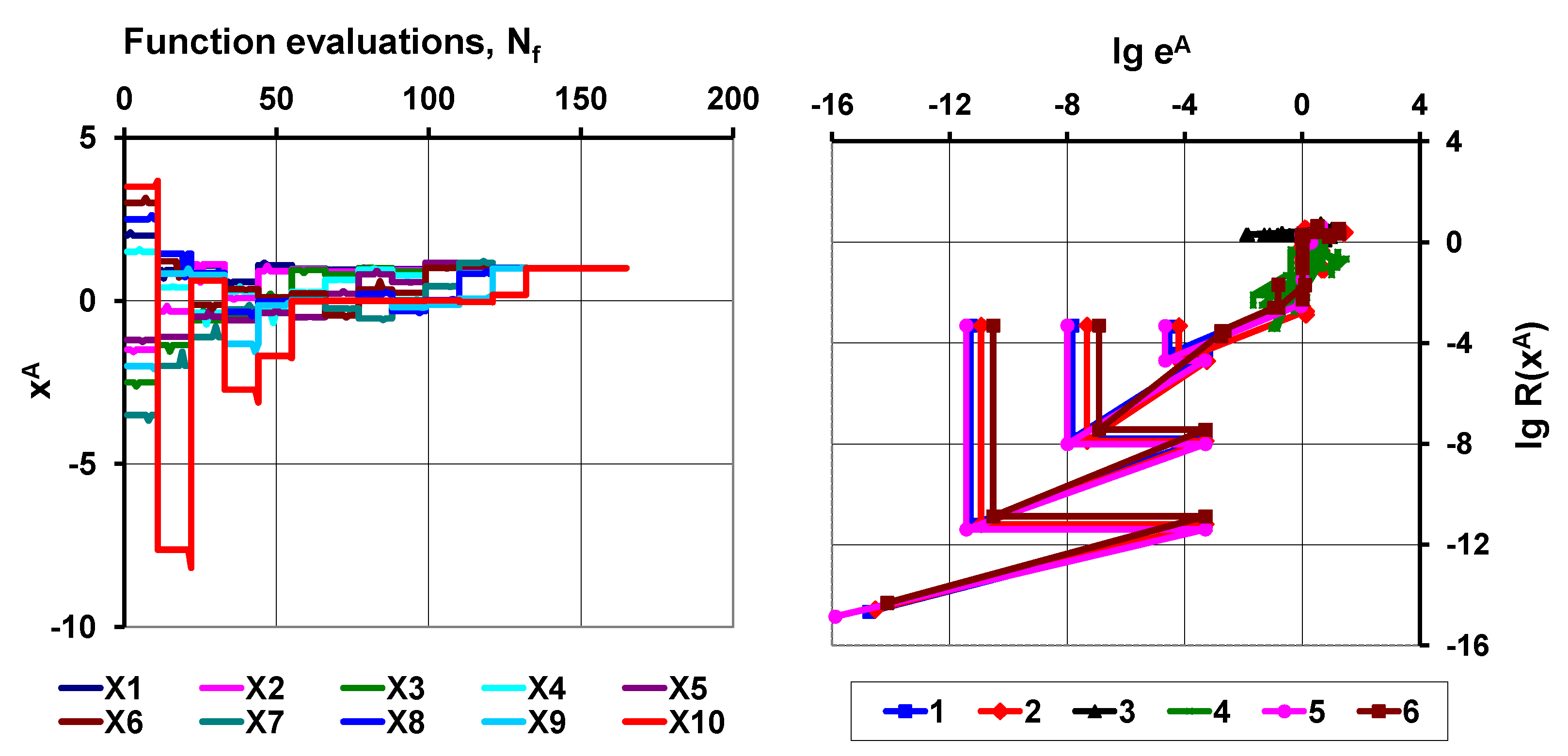
Let $N=n=10$ and $m=18$. Calculations were made with different, manually constructed initial trials ${\mathit{x}}_0^A=\left(x_{0,i}^A\right)$. Figure 12 (Left) shows the variation of $x_{p,i}^A$ for initial trial ${\mathit{x}}_0^A=$(2.0 −1.5 −2.5 1.5 −1.2 3.0 −3.5 2.5 −2.0 3.5). Iterations terminated after $N_f=154$ function evaluations ($p_{\mathit{max}}=14$ iterations) for the ${\epsilon }_p<{\epsilon }^{*}={10}^{-14}$ condition. Table 8 shows a set of further initial trials for numerical tests. Test “3” failed, probably due to the large distance from the global optimal solution. Test “4” found a local zero $x^{*}$ = $\left(-1111111111\right)$. Figure 12 (Right) summarizes the results of numerical tests “1–6”. The graphs show the iteration paths in the $lg\left|e_p^A\right|-R_p\left(x_p^A\right)$ plane. The graphs have an initial part, where the variation of $R_p\left(x_p^A\right)$ seems “chaotic”, while below $\left|e_p^A\right|\cong 0.01$ and $R_p\left(x_p^A\right)\cong 0.001$, the iterations run on similar paths.

Figure 12. $\left(\mathbf{Left}\right)$ Variation of $x_{p,i}^A$ for ${\mathit{x}}_0^A=\left(\begin{array}{cccccccccc}2.0& -1.5& -2.5& 1.5& -1.2& 3.0& -3.5& 2.5& -2.0& 3.5\end{array}\right)$ through iterations $\left(N=10=n=10,m=18\right)$ with $p_{\mathit{max}}=15$ and $N_f=165$. $\left(\mathbf{Right}\right)$ The absolute approximate errors $\mathit{lg}\left|e_p^A\left(x_{p,i}^A\right)\right|$$\left(i=1\dots 10\right)$ and the $R\left({\mathit{x}}_p^A\right)$ function variation through iterations for different initial trials $\left(N=10,n=10,m=18\right)$ (see Table 8).

Table 8. Initial trial vectors $\left(N=10,n=10,m=18\right)$, $\left({\mathit{x}}^{*}=\left(\begin{array}{ccc}1& \dots & 1\end{array}\right)\right)$.

	${\mathit{x}}_0^{\mathit{A}}$	${\mathit{p}}_{\mathit{max}}$	${\mathit{N}}_{\mathit{f}}$
1	$\left(\begin{array}{cccccccccc}1.3& -1.5& -2.1& 1.1& -1.3& 1.8& -1.8& 1.7& -2.0& 2.1\end{array}\right)$	15	165
2	$\left(\begin{array}{cccccccccc}3.1& -2.1& -4.3& 1.2& -2.4& 3.6& -1.6& 2.7& -4.2& 2.2\end{array}\right)$	21	231
3	$\left(\begin{array}{cccccccccc}-4.1& 1.1& -6.3& -3.2& -4.4& 1.6& 3.6& 5.7& -2.2& 3.2\end{array}\right)$	-	-
4	$\left(\begin{array}{cccccccccc}-3.0& -3.1& 2.3& -4.2& 2.4& -1.6& -3.6& 2.7& -2.2& 4.2\end{array}\right)$	-	-
5	$\left(\begin{array}{cccccccccc}2.1& 3.1& -1.3& -2.2& -3.4& 1.6& 2.6& -1.7& 2.2& -3.2\end{array}\right)$	16	176
6	$\left(\begin{array}{cccccccccc}3.1& 3.1& -4.3& -2.2& -3.4& 2.6& 1.6& -4.7& 2.2& -2.2\end{array}\right)$	20	220

9.3. Large $N\left(\begin{array}{ccc}200& 500& 1000\end{array}\right)$ Examples

A series of numerical tests has been performed with a large number of unknown variables. The values of the initial trials ${\mathit{x}}_0^A=\left(x_{0,i}^A\right),\left(i=1,\dots N\right)$ were generated as

$$x_{0,i}^A=x_i^{*}+L_1·\frac{Random-\frac{1}{2}}{5}+L_2,$$

(161)

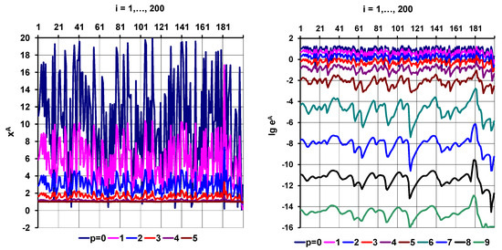
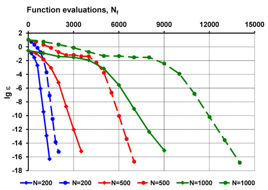
where “$\mathit{Random}$” is a random real number ($0\le \mathit{Random}<1$), and $L_i\left(i=1,2\right)$ are parameters regulating the size and location of the interval in which the initial trial values are expected to vary. ${\mathit{x}}^{*}=\left(x_i^{*}\right)=\left(\begin{array}{ccc}1& \dots & 1\end{array}\right)\left(i=1,\dots N\right)$ is the known global optimal solution. Table 9 shows the results of T-Secant iterations with $N=200$ and with initial trials ${\mathit{x}}_0^A: 0.1\le x_{0,i}^A\le 19.9$ ($L_1=99,L_2=9$). Figure 13 (Left) shows the variation of variables ${\mathit{x}}_p^A$ through T-Secant iterations. The iteration counter $p$ value is indicated below the graphs. Figure 13 (Right) shows the decrease in the approximate error ${\mathit{e}}_p^A=\left(e_{p,i}^A\right)$$\left(i=1,\dots ,200\right)$, with the $p$ iteration counter indication below the graphs. Table 10 shows the results of iterations with $N=1000$ and initial trials ${\mathit{x}}_0^A:0.5\le x_{0,i}^A\le 1.5$ ($L_1=5,L_2=0$). Figure 14 summarizes the results of numerical tests with a large number of unknowns $N=\left(\begin{array}{ccc}200& 500& 1000\end{array}\right)$. The norm ${\epsilon }_p$ of the approximate error ${\mathit{e}}_p^A$ decrease is shown, and the number of function value evaluations $N_f$ is indicated for $N=\left(\begin{array}{ccc}200\left(blue\right)& 500\left(red\right)& 1000\left(green\right)\end{array}\right)$ and for initial trials ${\mathit{x}}_0^A:0.5\le x_{0,i}^A\le 1.5$ (solid line) and ${\mathit{x}}_0^A:0.1\le x_{0,i}^A\le 19.9$ (dashed line).

Table 9. Iteration results ($N=200$, $L_1=99.9$, $L_2=9$) with initial trials $0.1\le x_{0,i}^A\le 19.9$ (dashed blue line on Figure 14).

$\mathit{p}$	${\mathit{\epsilon }}_{\mathit{p}}$	$\mathit{R}\left({\mathit{x}}_{\mathit{p}}^{\mathit{A}}\right)$	${\mathit{N}}_{\mathit{f}}$
0	10.6925833405791	24123.43773726327	1
1	5.45917411911925	6895.1103569982861	201
2	2.13338434746463	1247.4064173528971	402
3	0.71430571273689	220.36900527956962	603
4	0.163511639031299	32.621494717337107	804
5	0.0145616620270659	2.4077509738413969	1005
6	0.000197003511771894	0.026366233831030046	1206
7	0.000000084768909602	0.000007982826913871	1407
8	0.000000000032791210	0.000000003114429023	1608
9	0.000000000000013862	0.000000000001333830	1809
10	0.000000000000000546	0.000000000000104185	2010

Figure 13. $\left(\mathbf{Left}\right)$ Variation of variables ${\mathit{x}}_p^A$ through iterations. $\left(\mathbf{Right}\right)$ Decrease in approximate error $lg{e}_p^A$ through iterations, $N=200$ (with iteration counter $p$ value indication below the graphs).

Table 10. Iteration results ($N=1000,L_1=5,L_2=0$) with initial trials $0.5\le x_{0,i}^A\le 1.5$ (solid green line on Figure 14).

$\mathit{p}$	${\mathit{\epsilon }}_{\mathit{p}}$	$\mathit{R}\left({\mathit{x}}_{\mathit{p}}^{\mathit{A}}\right)$	${\mathit{N}}_{\mathit{f}}$
0	0.287800987765134	212.38512786560364	1
1	0.121219403643695	57.87378211356512	1001
2	0.0396263348376487	13.743840511211417	2002
3	0.0298060844365720	9.6618077142097238	3003
4	0.0120370539008435	5.9465782106406841	4004
5	0.000705489922936629	0.42465246853444877	5005
6	0.000002762586723754	0.001324115254348589	6006
7	0.000000000990421380	0.000000388965253003	7007
8	0.000000000000433209	0.000000000155930410	8008
9	0.000000000000000860	0.000000000000363149	9009

Figure 14. Number of function evaluations for $N=200$ (blue), $N=500$ (red), and $N=1000$ (green) with initial trials ${\mathit{x}}_0^A:0.5\le x_{0,i}^A\le 1.5$ (solid line) and ${\mathit{x}}_0^A:0.1\le x_{0,i}^A\le 19.9$ (dashed line).

10. Efficiency

10.1. Single-Variable Case

The efficiency of an algorithm relates to the amount of computational resources used by the algorithm. For better efficiency, it is desirable to minimize resource usage. An algorithm is considered efficient if its resource consumption (computational cost) is below some acceptable level (it runs in a reasonable amount of time or space on an available computer). The efficiency of an algorithm for the solution of nonlinear equations is thoroughly discussed by Traub [25] as follows. Let $p$ be the order of the iteration sequence such that for the approximate errors $e_i=x_i-x^{*}$, there exists a nonzero constant $C$ (asymptotic error constant) for which

$$\frac{\left|e_{i+1}\right|}{{\left|e_i\right|}^p}\to C.$$

(162)

A natural measure of the information used by an algorithm is the “informational usage” $d$, which is defined as the number of new pieces of information (values of the function and its derivatives) required per iteration (called “horner” by Ostrowski [26]). Then, the efficiency of the algorithm within one iteration can be measured by the “informational efficiency”:

$$EFF=\frac{p}{d}.$$

(163)

An alternative definition of efficiency is

$${}^{*}\mathit{EFF}=p^{\frac{1}{d}},$$

(164)

called the “efficiency index” by Ostrowski [26]. Another measure of efficiency, called “computational efficiency”, takes into account the “cost” of calculating different derivatives. The concept of informational efficiency ($\mathit{EFF}$) and the efficiency index (${}^{*}\mathit{EFF}$) do not take into account the cost of evaluating $f$ and its derivatives, nor do they take into account the total number of pieces of information needed to achieve a certain accuracy in the root of the function. If $f$ is composed of elementary functions, then the derivatives are also composed of elementary functions; thus, the cost of evaluating the derivatives is merely the cost of combining the elementary functions. Table 11 compares the efficiencies of classic (secant, Newton) and improved algorithms (T-Secant, T-Newton).

Table 11. Efficiencies of classic and improved algorithms.

Method	$\mathit{d}$	$\mathit{p}$	$\mathit{EFF}$ [25]	${}^{*}\mathit{EFF}$ [26]
Secant	1	$1.618\dots$	$1.618\dots$	$1.618\dots$
Newton	2	$2.0$	$1.0$	$1.414\dots$
T-Secant	2	$2.618\dots$	$1.309\dots$	$1.618\dots$
T-Newton	3	$3.0$	$1.0$	$1.442\dots$

10.2. Multi-Variable Case

Very limited data are available to compare the performance of the T-Secant method with other methods, especially in cases with a large number of unknowns. Broyden [27] suggested the mean convergence rate

$$L=\frac{1}{N_f}ln\frac{R\left(x_0^A\right)}{R\left(x_{p_{max}}^A\right)}$$

(165)

as a measure of efficiency of an algorithm for solving a particular problem, where $N_f$ is the total number of function evaluations, $x_0^A$ is the initial trial, and $x_{p_{\mathit{max}}}^A$ is the last trial for the solution $x^{*}$ when the termination criteria is satisfied after $p_{\mathit{max}}$ iterations. $R\left(x\right)$ is the Euclidean norm of $\mathit{f}\left(x\right)$. Efficiency results were given by Broyden [27] for the Rosenbrock function for $N=2$ and for ${\mathit{x}}_0^A=\left(\begin{array}{cc}-1.2& 1.0\end{array}\right)$. The calculated convergence rates for the two Broyden method variants [27], for the Powell’s method [28], for the adaptive coordinate descent method [29] m and for the Nelder–Mead simplex method [30] were compared with the calculated values for the T-Secant method in Table 12. Rows 1–5 are data from referenced papers, rows 6–8 are T-Secant results with the referenced initial trials, and rows 9–15 are calculated data for $N>2$.

Table 12. Calculated values of the mean convergence rates ($L$ and $L_N$) for the Rosenbrock function (${ }^1$: a substitute value ${10}^{-25}$ was used when $R\left({\mathit{x}}_{p_{\mathit{max}}}^A\right)=0$).

	$\mathit{N}$	Method	$\mathit{R}\left({\mathit{x}}_0^{\mathit{A}}\right)$	$\mathit{R}\left({\mathit{x}}_{{\mathit{p}}_{\mathit{max}}}^{\mathit{A}}\right)$	${\mathit{p}}_{\mathit{max}}$	${\mathit{N}}_{\mathit{f}}$	$\mathit{L}$	${\mathit{L}}_{\mathit{N}}$
1	2	Broyden 1. [27]	4.9193	4.73 × 10$-1$	-	59	0.391	0.78
2	2	Broyden 2. [27]	4.9193	2.55 × 10−1	-	39	0.607	1.22
3	2	Powell [28]	4.9193	7.00 × 10 $-1$	-	151	0.150	0.30
4	2	ACD [29]	130.062	1.00 × 10$-1$	-	325	0.086	0.17
5	2	Nelder-Mead [30]	2.0000	1.36 × 10$-1$	-	185	0.127	0.25
6	2	T-secant [27,28]	4.9193	1.0 × 10−25 1	3	9	6.573 1	13.15 1
7	2	T-secant [29]	130.06	1.0 × 10−25 1	3	9	6.937 1	13.87 1
8	2	T-secant [30]	2.0000	6.66 × 10−15	2	6	5.556	11.11
9	3	T-secant	72.722	1.41 × 10−14	5	20	1.809	5.43
10	3		32.466	1.0 × 10−25 1	4	16	3.815 1	11.45 1
11	5		93.528	1.34 × 10−14	8	48	0.760	3.80
12	5		7.193	5.90 × 10−14	4	24	1.351	6.76
13	10		202.62	1.0 × 10−25 1	14	154	0.408 1	4.08 1
14	200		92.778	9.00 × 10$-15$	10	2010	0.042	8.44
15	1000		212.39	3.63 × 10$-13$	6	6006	0.006	5.66

Results show that the mean convergence rate $L$ (Equation (165)) for $N=2$ is much higher for the T-Secant method ($\simeq 5.5–6.9$) than for the other listed methods ($\simeq 0.1–0.6$); however, it is obvious that the mean convergence rate values decrease rapidly with increasing $N$ values (more unknowns need more function evaluations). A modified convergence rate

$$L_N=N\ast L=\frac{N}{N_f}\ln \frac{R\left({\mathit{x}}_0^A\right)}{R\left({\mathit{x}}_{p_{\mathit{max}}}^A\right)}$$

(166)

can be used as an $“N”$ independent measure of efficiency (see Table 12). The values of $L$ and $L_N$ are at least 10 times larger for the T-Secant method than for the referenced classic methods for $N=2$ (see Table 12). Note that the efficiency measures ($L$ and $L_N$) are also dependant on the initial conditions (distance of the initial trial set from the optimal solution, termination criterion). Results from a large number of numerical tests indicate an average $L_N$ value of around $7.4$, with standard deviation $3.7$ for the T-Secant method even for large $N$ values. It has to be noted that if the value of $R\left({\mathit{x}}_{p_{\mathit{max}}}^A\right)$ is zero, then the mean convergence rates ($L$ and $L_N$) are not countable (zero in the denominator). A substitute value ${10}^{-25}$ was used when iterations ended with $R\left({\mathit{x}}_{p_{\mathit{max}}}^A\right)=0$ in the sample examples.

11. Discussions

11.1. General

The suggested procedure needs the usual approximate $x_{p+1}^A$ to be determined by any of a classic quasi-Newton iterative methods (Wolfe–Popper–Secant, Broyden, etc.). By using the “information” $f_{p+1}^A$, an additional and independent approximate $x_{p+1}^B$ is determined, which provides the possibility for a full-rank update of the approximate derivatives (${\mathit{S}}_p$ for Secant or ${\mathit{B}}_p$ for Broyden). Results and experience show that the suggested procedure considerably accelerates the convergence and the efficiency of the classic methods, and the full-rank update technique increases the stability of the iterative procedure. In multi-variable-case, it follows from Equation (107) that

$${\left({\mathit{T}}_p^X\right)}^{-1}▵{\mathit{x}}_p^A=-{\mathit{S}}_p^{+}{\left({\mathit{T}}_p^F\right)}^{-1}{\mathit{f}}_p^A,$$

(167)

and in explicit form after re-arrangement:

$$\left[\frac{{\left(▵x_{p,i}^A\right)}^2}{x_{p+1,i}^B-x_{p+1,i}^A}\right]=-\left[S_{p,i,j}^{+}\right]\left[\frac{f_{p,j}^A}{t_{p,j}^F}\right].$$

(168)

Then, the $i^{\mathit{th}}$ element of the new approximate ${\mathit{x}}_{p+1}^B$ can be expressed from the $i^{\mathit{th}}$ row of the above equation as

$$x_{p+1,i}^B=x_{p+1,i}^A-\frac{{\left(▵x_{p,i}^A\right)}^2}{{\displaystyle \sum _{j=1}^m}\left(S_{p,i,j}^{+}\frac{f_{p,j}^A}{t_{p,j}^F}\right)}.$$

(169)

The mechanism of the procedure resembles to the mechanism of an engine’s turbocharger that is powered by the flow of exhaust gases (analogous to $f_{p+1}^A$ or $t_{p,j}^F$).

11.2. Newton Method

Matrix $\mathit{S}$ in the general formula (104) gives a direct connection between the Secant and Newton methods, as differences go to differentials,

$$\mathit{S}=\left[\frac{▵f_{k,j}}{▵x_i}\right]=\left[S_{i,j}\right]⟶\mathit{J}=\left[\frac{\partial f_{k,j}}{\partial x_i}\right]=\left[J_{i,j}\right]$$

(170)

where $\mathit{J}$ is the Jacobian matrix of the function $\mathit{f}:{\mathbb{R}}^n\to {\mathbb{R}}^m$ ($m\ge n$) with $k$ and $i$ column and with $j$ row indexes, respectively. It follows from formula (111) of matrix ${\mathit{S}}_T$ that the suggested full-rank update procedure can also be applied to the Newton method as

$${\mathit{S}}_T=\left[\frac{t_j^F}{t_i^X}\frac{▵f_{k,j}}{▵x_i}\right]⟶{\mathit{J}}_T=\left[\frac{t_j^F}{t_i^x}\frac{\partial f_{k,j}}{\partial x_i}\right],$$

(171)

where ${\mathit{J}}_T$ is the modified Jacobian matrix of the “T-Newton” method. In the single-variable case, with approximate $x_p^A$ in the $p^{\mathit{th}}$ iteration, with function value $f_p^A=f\left(x_p^A\right)$ and with derivative function value $f_p^{\prime A}=f^{\prime }\left(x_p^A\right)$, the new Newton–Raphson approximate can be expressed as

$$x_{p+1}^A=x_p^A-\frac{\partial x_p}{\partial f_p}{f}_p^A=x_p^A-\frac{f_p^A}{f_p^{\prime A\prime }}$$

(172)

and the iteration stepsize is

$$▵x_p^A=x_{p+1}^A-x_p^A$$

(173)

with the hyperbolic function (Equation (88))

$$z_p\left(x\right)=\frac{a_p}{x-x_{p+1}^A}+f_p^A.$$

(174)

where

$$a_p={\left(x_{p+1}^A-x_p^A\right)}^2{f}_p^{\prime A}\frac{f_{p+1}^A}{f_p^A}$$

(175)

($▵f_p/▵x_p$ is replaced by $f_p^{\prime A}$), the new “T-Newton” approximate is

$$x_{p+1}^B=x_{p+1}^A-\frac{{\left(▵x_p^A\right)}^2{f}_p^{\prime A}{f}_{p+1}^A}{{\left(f_p^A\right)}^2}$$

(176)

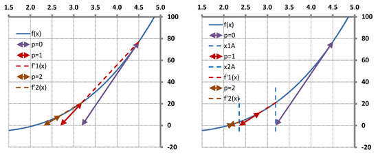
($▵f_p/▵x_p$ is again replaced by $f_p^{\prime A}$), similar to Equation (59) in case of the T-secant method. It can be seen from Table 13 and Table 14 that the convergence rate is be improved from ${\alpha }^N=2$ to ${\alpha }^{TN}=3$. In the multi-variable case, it follows from Equation (107) (${\mathit{S}}_p^{+}$ is replaced by ${\mathit{J}}_p^{+}$) that

$${\left({\mathit{T}}_p^X\right)}^{-1}▵{\mathit{x}}_p^A=-{\mathit{J}}_p^{+}{\left({\mathit{T}}_p^F\right)}^{-1}{\mathit{f}}_p^A$$

(177)

and in explicit form after re-arrangement:

$$\left[\frac{{\left(▵x_{p,i}^A\right)}^2}{x_{p+1,i}^B-x_{p+1,i}^A}\right]=-\left[J_{p,i,j}^{+}\right]\left[\frac{f_{p,j}^A}{t_{p,j}^F}\right].$$

(178)

Then, the $i^{\mathit{th}}$ element of the new “T-Newton” approximate ${\mathit{x}}_{p+1}^B$ can be expressed from the $i^{\mathit{th}}$ row of the above equation as

$$x_{p+1,i}^B=x_{p+1,i}^A-\frac{{\left(▵x_{p,i}^A\right)}^2}{{\displaystyle \sum _{j=1}^m}\left(J_{p,i,j}^{+}\frac{f_{p,j}^A}{t_{p,j}^F}\right)},$$

(179)

similar to Equation (70) in case of the T-Secant method. Thus, the “hyperbolic” approximation accelerates the convergence of the Newton=-Raphson method by only one additional function evaluation.

Table 13. Newton method iteration and computed convergence rate, ${\alpha }^N$.

$\mathit{p}$	${\mathit{x}}_{\mathit{p}}^{\mathit{A}}$	${\mathit{x}}_{\mathit{p}+1}^{\mathit{A}}$	$\left|{\mathit{e}}_{\mathit{p}+1}^{\mathit{A}}\right|$	${\mathit{\alpha }}^{\mathit{N}}$	${\mathit{N}}_{\mathit{f}}$	${\mathit{N}}_{{\mathit{f}}^{\prime }}$
0	4.5	3.187	$1.1\times {10}^0$		1	1
1	3.187	2.44965	$3.6\times {10}^{-1}$		2	2
2	2.44965	2.14996	$5.5\times {10}^{-2}$	1.42	3	3
3	2.14996	2.096188	$1.6\times {10}^{-3}$	1.66	4	4
4	2.096188	2.094552	$1.5\times {10}^{-6}$	1.89	5	5
5	2.094552	2.09455148	$1.3\times {10}^{-12}$	1.99	6	6
6	2.09455148	2.09455148154233	$3.6\times {10}^{-15}$	2.00	7	7

Table 14. T-Newton method iteration and computed convergence rate, ${\alpha }^{TN}$ (see Figure 15).

$\mathit{p}$	${\mathit{x}}_{\mathit{p}}^{\mathit{A}}$	${\mathit{x}}_{\mathit{p}+1}^{\mathit{B}}$	$\left|{\mathit{e}}_{\mathit{p}+1}^{\mathit{B}}\right|$	${\mathit{\alpha }}^{\mathit{TN}}$	${\mathit{N}}_{\mathit{f}}$	${\mathit{N}}_{{\mathit{f}}^{\prime }}$
0	4.5	2.830	$7.4\times {10}^{-1}$		2	1
1	2.830	2.17760	$8.3\times {10}^{-2}$		4	2
2	2.17760	2.09486	$3.1\times {10}^{-4}$	1.84	6	3
3	2.09486	2.09455148	$1.9\times {10}^{-11}$	2.56	8	4
4	2.09455148	2.09455148154233	$3.6\times {10}^{-15}$	2.97	9	5

Figure 15. T-Newton iterations with test function (99) with initial approximate $x_0^A=4.5$. $\mathbf{Left}$: $x_1^B$ is the root of the tangent line through $f_0^{\prime A}$, $x_1^A$ is the root of $z_0\left(x\right)$. $\mathbf{Right}$: $x_2^B$ is the root of the tangent line through $f_1^{\prime A}$; $x_2^A$ is the root of $z_1\left(x\right)$ (see data in Table 14).

Table 14. T-Newton method iteration and computed convergence rate, ${\alpha }^{TN}$ (see Figure 15).

$\mathit{p}$	${\mathit{x}}_{\mathit{p}}^{\mathit{A}}$	${\mathit{x}}_{\mathit{p}+1}^{\mathit{B}}$	$\left|{\mathit{e}}_{\mathit{p}+1}^{\mathit{B}}\right|$	${\mathit{\alpha }}^{\mathit{TN}}$	${\mathit{N}}_{\mathit{f}}$	${\mathit{N}}_{{\mathit{f}}^{\prime }}$
0	4.5	2.830	$7.4\times {10}^{-1}$		2	1
1	2.830	2.17760	$8.3\times {10}^{-2}$		4	2
2	2.17760	2.09486	$3.1\times {10}^{-4}$	1.84	6	3
3	2.09486	2.09455148	$1.9\times {10}^{-11}$	2.56	8	4
4	2.09455148	2.09455148154233	$3.6\times {10}^{-15}$	2.97	9	5

11.3. Broyden’s Method

Broyden’s method is a special case of the Secant method. In the single-variable case, the derivative of the function is approximated as

$$f_p^{\prime }\simeq B_p=B_{p-1}+\frac{▵f_p-B_{p-1}▵x_p}{{\left|▵x_p\right|}^2}▵x_p$$

(180)

in the $p^{\mathit{th}}$ iteration step, and with

$$\frac{▵x_p}{{\left|▵x_p\right|}^2}=\frac{1}{▵x_p}$$

(181)

it is simplified as

$$B_p=B_{p-1}+\frac{▵f_p-B_{p-1}▵x_p}{▵x_p}.$$

(182)

The next Broyden-approximate is then determined as

$$x_{p+1}^A=x_p^A-\frac{f_p^A}{B_p}.$$

(183)

The convergence can similarly be improved by the new hyperbolic approximation procedure as in cases of the Secant and Newton methods. An additional new approximate

$$x_{p+1}^B=x_{p+1}^A-\frac{{\left(▵x_p^A\right)}^2{B}_p{f}_{p+1}^A}{{\left(f_p^A\right)}^2}$$

(184)

can be determined, and the iteration continues with this value. Figure 16 demonstrates the effect of the hyperbolic approximation applied to the classic Broyden method. Not surprisingly, the convergence rate will be improved from ${\alpha }^B=\phi \simeq 1.618$ to ${\alpha }^{TB}={\phi }^2\simeq 2.618$, as in case of the Secant method. In the multi-variable case, the $i^{\mathit{th}}$ element of the new the “T-Broyden” approximate ${\mathit{x}}_{p+1}^B$ can be expressed as

$$x_{p+1,i}^B=x_{p+1,i}^A-\frac{{\left(▵x_{p,i}^A\right)}^2}{{\displaystyle \sum _{j=1}^m}\left(B_{p,i,j}^{+}\frac{f_{p,j}^A}{t_{p,j}^F}\right)},$$

(185)

similar to Equation (179) for the T-Newton method with $J_{p,i,j}^{+}$ replaced by $B_{p,i,j}^{+}$. The new approximate $B_{p+\mathit{1}}$ to the Jacobian matrix can then be fully updated in a similar way as it was in the case of the T-Secant method.

Figure 16. Broyden ($\mathbf{Left}$) and T-Broyden ($\mathbf{Right}$) iterations with test function (99) with initial approximates $x_0^A=4.5$.

12. Conclusions

A completely new iteration strategy has been worked out for solving simultaneous nonlinear equations:

$$\mathit{f}\left(\mathit{x}\right)=0,$$

(186)

$\mathit{x}\in$${\mathbb{R}}^n$, and $\mathit{f}:{\mathbb{R}}^n\to {\mathbb{R}}^m$ ($m\ge n$). It replaces the Jacobian matrix with finite-difference approximations. The stepsize $▵x_{p+1}$ was determined as the difference between two new approximates

$${\mathit{x}}_{p+1}^A={\mathit{x}}_p^A+▵{\mathit{x}}_p^A$$

(187)

and ${\mathit{x}}_{p+\mathit{1}}^B$ with elements

$$x_{p+1,i}^B=x_{p+1,i}^A+▵x_{p+1,i}=x_{p+1,i}^A-\frac{{\left(▵x_{p,i}^A\right)}^2}{{\displaystyle \sum _{j=1}^m}\left(S_{p,i,j}^{+}\frac{f_{p,j}^A}{t_{p,j}^F}\right)}$$

(188)

$\left(i=1,\dots ,n\right)$ as

$$▵{\mathit{x}}_{p+1}={\mathit{x}}_{p+1}^B-{\mathit{x}}_{p+1}^A.$$

(189)

The first one is a classic quasi-Newton approximate with stepsize $▵{\mathit{x}}_p^A$, while the second one was determined from a hyperbolic approximation governed by ${\mathit{x}}_{p+1}^A$ and ${\mathit{f}}_{p+1}^A$, such that the classic Secant equation

$$\mathit{S}▵{\mathit{x}}^A=-{\mathit{f}}^A$$

(190)

was modified by a non-uniform scaling transformation

$$\mathit{T}=\left[\begin{array}{cc}{\mathit{T}}^X& \mathbf{0}\\ \mathbf{0}& {\mathit{T}}^F\end{array}\right]$$

(191)

with diagonal elements $t_j^F$$\left(j=1,\dots ,m\right)$, $t_i^X$$\left(i=1,\dots ,n\right)$ as

$${\mathit{S}}_T▵{\mathit{x}}^A=-{\mathit{f}}^A,$$

(192)

where

$$\mathit{S}=\left[\frac{▵f_{k,j}}{▵x_i}\right]\mathit{and}{\mathit{S}}_T=\left[\frac{t_j^F}{t_i^X}\frac{▵f_{k,j}}{▵x_i}\right]$$

(193)

$\left(k=1,\dots ,\mathit{n}\right)$. It was shown that the new stepsize $▵{\mathit{x}}_{p+1}$ is much smaller than the stepsize $▵{\mathit{x}}_p^A$ of the classic quasi-Newton approximate, providing that ${\mathit{x}}_{p+1}^B$ will always be in the vicinity of ${\mathit{x}}_{p+1}^A$. Having two new approximates, a set of $n+1$ new independent trial approximates ${\mathit{x}}_{p+1}^A$ and ${\mathit{x}}_{k,p+1}^B$ $\left(k=1,\dots ,n\right)$ was constructed (see Equation (32)), providing that the new trial approximates are always in general positions, ensuring the stable behavior of the iteration. According to the geometrical representation in the single-variable case, the suggested procedure corresponds to finding the root of a hyperbolic function with vertical and horizontal asymptotes $x_{p+1}^A$ and $f_p^A$. It was shown in Section 7 that the suggested method has super-quadratic convergence with a rate of ${\alpha }^{TS}=$${\phi }^2=2.618\dots$(where $\phi =1.618\dots$ is the well-known golden ratio) in the single-variable case.

The suggested method needs two function evaluations in each iteration in single-variable cases and $n+1$ evaluations in multi-variable cases. The efficiency of the proposed method was studied in Section 10 in the multi-variable case and compared with other classic low-rank-update and line-search methods on the basis of available data. The results show that the efficiency of the suggested full-rank-update procedure is considerably better than the efficiency of the other referenced methods. A Rosenbrock test function (Equations (158) and (159)) with up to $n=1000$ variables was used to demonstrate this efficiency in Section 9.

References

- Rüth, B.; Uekermann, B.; Mehl, M.; Birken, P.; Monge, A.; Bungartz, H.-J. Quasi-Newton waveform iteration for partitioned surface-coupled multiphysics applications. Int. J. Numer. Methods Eng. 2021, 122, 5236–5257. [Google Scholar] [CrossRef] [Scilit]
- Barnafi, N.A.; Pavarino, L.F.; Scacchi, S. Parallel inexact Newton-Krylov and quasi-Newton solvers for nonlinear elasticity. Comput. Methods Appl. Mech. Engrg. 2022, 400, 115557. [Google Scholar] [CrossRef] [Scilit]
- Ryu, J.; Jae, M. A quantification methodology of Seismic Probabilistic Safety Assessment for nuclear power plant. Ann. Nucl. Energy 2021, 159, 108296. [Google Scholar] [CrossRef] [Scilit]
- Yahaya, M.M.; Kumam, P.; Awwal, A.M.; Aji, S. A structured quasi-Newton algorithm with nonmonotone search strategy for structured NLS problems and its application in robotic motion control. J. Comput. Appl. Math. 2021, 395, 113582. [Google Scholar] [CrossRef] [Scilit]
- Schröter, M.; Sauer, O. Quasi-Newton Algorithms for Medical Image Registration. In Proceedings of the World Congress on Medical Physics and Biomedical Engineering, Munich, Germany, 7–12 September 2009; Dössel, O., Schlegel, W.C., Eds.; IFMBE Proceedings. Springer: Berlin/Heidelberg, Germany, 2019; Volume 25/4. [Google Scholar] [CrossRef] [Scilit]
- Ludwig, A. The Gauss–Seidel–quasi-Newton method: A hybrid algorithm for solving dynamic economic models. J. Econ. Dyn. Control. 2007, 31, 1610–1632. [Google Scholar] [CrossRef] [Scilit]
- Wülfingen, G.B. On some advantages of the application of Newton’s method for the solution of nonlinear economic models. In Proceedings of the IFAC Dynamic Modelling, Warsaw, Poland, 16–19 June 1980; pp. 339–347. [Google Scholar]
- Schaefer, B.; Ghasemi, S.A.; Roy, S.; Goedecker, S. Stabilized quasi-Newton optimization of noisy potential energy surfaces. J. Chem. Phys. 2015, 142, 034112. [Google Scholar] [CrossRef] [Scilit] [PubMed]
- Kemeny, J.G.; Snell, J.L. Mathematical Models in the Social Sciences. Introduction to Higher Mathematics; Blaisdell Publishing Company, A Division of Ginn and Company: New York, NY, USA; Toronto, ON, Canada; London, UK, 1963; Volume VII, 145p. [Google Scholar]
- Beregi, S.; Barton, D.A.W.; Rezgui, D.; Nield, S.A. Real-Time Hybrid Testing Using Iterative Control for Periodic Oscillations, arXive. Available online: https://arxiv.org/abs/2312.06362 (accessed on 15 December 2023).
- Barnafi, N.A.; Pavarino, L.F.; Scacchi, S. Parallel inexact Newton-Krylov and Quasi-Newton Solvers for Nonlinear Elasticity, arXive. Available online: https://arxiv.org/abs/2203.05610 (accessed on 15 December 2023).
- Ortega, J.M.; Rheinboldt, W.C. Iterative Solution of Nonlinear Equations in Several Variables; Academic Press: New York, NY, USA, 1970. [Google Scholar]
- Dennis, J.E., Jr.; Schnabel, R.B. Numerical Methods for Unconstrained Optimization and Nonlinear Equations; Prentice-Hall: Englewood Cliffs, NJ, USA, 1983. [Google Scholar]
- Stoer, J.; Bulirsch, R. Introduction to Numerical Analysis, 3rd ed.; Springer: Berlin/Heidelberg, Germany, 2002. [Google Scholar]
- Martinez, J.M.; Qi, L. Inexact Newton methods for solving nonsmooth equations. J. Comput. Appl. Math. 1995, 60, 127–145. [Google Scholar] [CrossRef] [Scilit]
- Dembo, R.S.; Eisenstat, S.C.; Steihaug, T. Inexact Newton methods. SIAM J. Numer. Anal. 1971, 19, 400–408. [Google Scholar] [CrossRef] [Scilit]
- Birgin, E.G.; Krejic, N.; Martinez, J.M. Globally convergent inexact quasi-Newton methods for solving nonlinear systems. Num. Algorithms. 2003, 32, 249–260. [Google Scholar] [CrossRef] [Scilit]
- Martínez, J.M. Practical quasi-Newton methods for solving nonlinear systems. J. Comput. Applied Math. 2000, 124, 97–121. [Google Scholar] [CrossRef] [Scilit]
- Wolfe, P. The Secant Method for Simultaneous Nonlinear Equations. Commun. ACM 1959, 2, 12–13. [Google Scholar] [CrossRef] [Scilit]
- Popper, G. Numerical method for least square solving of nonlinear equations. Period. Polytech. 1985, 29, 67–69. [Google Scholar]
- Berzi, P. Model investigation for pile bearing capacity prediction. In Proceedings of the Euromech (280) Symposium on Identification of Nonlinear Mechanical Systems from Dynamic Tests, Ecully, France, 29–31 October 1991. [Google Scholar]
- Berzi, P. Pile-Soil Interaction due to Static and Dynamic Load. In Proceedings of the XIII ICSMFE, New Delhi, India, 5–10 January 1994; pp. 609–612. [Google Scholar]
- Berzi, P.; Beccu, R.; Lundberg, B. Identification of a percussive drill rod joint from its response to stress wave loading. Int. J. Impact Eng. 1994, 18, 281–290. [Google Scholar] [CrossRef] [Scilit]
- Rosenbrock, H.H. An automatic Method for finding the Greatest or Least Value of a Function. Comput. J. 1960, 3, 175–184. [Google Scholar] [CrossRef] [Scilit]
- Traub, J.F. Iterative Methods for the Solution of Equations, 1st ed.; Prentice-Hall, Inc.: Englewood Cliffs, NJ, USA, 1964. [Google Scholar]
- Ostrowski, A.M. Solution of Equations and Systems of Equations; Academic Press: New York, NY, USA, 1966. [Google Scholar]
- Broyden, C.G. A class of Methods for Solving Nonlinear Simultaneous Equations. Math. Comput. Am. Math. 1965, 19, 577–593. [Google Scholar] [CrossRef]
- Powell, M.J.D. An efficient method for finding the minimum of a function of several variables without calculating derivatives. Comput. J. 1964, 7, 155–162. [Google Scholar] [CrossRef] [Scilit]
- Loshchilov, I.; Schoenauer, M.; Sebag, M. Adaptive Coordinate Descent. In Proceedings of the Genetic and Evolutionary Computation Conference (GECCO), Dublin, Ireland, 12–16 July 2011; ACM Press: New York, NY, USA, 2011; pp. 885–892. [Google Scholar]
- Nelder, J.A.; Mead, R. A simplex method for function minimization. Comput. J. 1965, 7, 308–313. [Google Scholar] [CrossRef] [Scilit]
Disclaimer/Publisher’s Note: The statements, opinions and data contained in all publications are solely those of the individual author(s) and contributor(s) and not of MDPI and/or the editor(s). MDPI and/or the editor(s) disclaim responsibility for any injury to people or property resulting from any ideas, methods, instructions or products referred to in the content. |
© 2024 by the author. Licensee MDPI, Basel, Switzerland. This article is an open access article distributed under the terms and conditions of the Creative Commons Attribution (CC BY) license (https://creativecommons.org/licenses/by/4.0/).