Machine-Learning-Based Design Optimization of Chassis Bushings

Abstract

In this work, a method is developed for the component design of chassis bushings with contoured inner cores, aided by artificial neural networks (ANNs) and design optimization. First, a model of a physical chassis bushing is generated using the finite element method (FEM). To determine the material parameters of the material model, a material parameter optimization is conducted. Based on the bushing model, different samples for a design study are generated using the design of experiments method. Due to invalid areas of the geometrical model definitions, constraints are established and the design parameter space is cleaned up. From the cleaned design parameter space, a database of several design parameter samples and three associated quasi-static stiffnesses, calculated with FEM simulations, is generated. The database is subsequently used for the training and hyper-parameter optimization of the ANN. Subsequently, the feed-forward ANN is employed in a design study, where stiffnesses are prescribed and design parameters identified. The design process is inverted with the help of a constrained design parameter optimization (DO), based on particle swarm optimization (PSO). Two usecases are defined for the evaluation of the design accuracy of the entire method. The design parameters found are validated by corresponding FEM simulations.

1. Introduction

The vehicle development process is subject to strong competitive pressure because of the continuously increasing number of vehicle derivatives and shorter vehicle development cycles [1]. Aggressive new players with innovative technologies and progressing digitalization in the automotive industry are causing further challenges for vehicle manufacturers [2].

According to Klostermeier [3], the use of digital twins is important for the automotive industry as increasingly efficient and faster product development with a simultaneous reduction in real prototypes helps to reduce costs and development time.

The full vehicle specifications defined at the beginning of the vehicle development process from the domains of ride comfort, driving dynamics, acoustics, and so forth often lead to component requirements at the component level with a high demand on design and material selection [4]. With the use of digital twins in the development process, it is possible to generate design concepts at an early phase and use them to make virtual estimates of the required installation space as well as forecasts of the target value fulfillment.

Specifically, the design of elastomeric bearings is important for achieving the required full-vehicle characteristics. The vibration-isolating behavior based on the viscoelastic characteristics of elastomers helps to reduce vibrations and noise from engine-, transmission-, and road-induced vibrations [4]. In addition, elastomeric bearings (chassis bushings) in the chassis contribute significantly to the elasto-kinematic characteristics of the wheel control. The design of the compliance of chassis bushings helps to adjust wheel position values under the action of forces [4].

Due to the nonlinear material behavior of rubber [4], the design of the component behavior is very demanding and requires robust virtual calculation and simulation methods.

Adkins [5] and Göbel [6] have already developed analytical calculation models for the stiffnesses of cylindrical bushings at radial, axial, and torsional deformation. They assumed linear elastic material behavior for quasi-static deformation of the elastomer material. Their calculation models are based on cylindrical bushings with a constant cross-section.

The validity of analytical calculation models based on linear elastic material behavior has been investigated in a previous study [7] that considered eight simple bushings (cylinders with constant cross-section) with different design parameters. The mean relative deviation of the calculated to the measured static stiffness was 10% for radial deformation.

Bushings in modern vehicles are subject to strong requirements. To fulfill the target values, it is often necessary to use component designs that deviate significantly from simple bushings with constant cross-sections. Complex component designs (e.g., contoured inner sleeves) lead to an inhomogeneous stress distribution in the elastomer material and require numerical methods [4,8].

For the design of elastomer components with complex geometries, the finite element method (FEM) is usually used. This method enables the variation of individual model parameters (e.g., geometry parameters) and the calculation of the mechanical properties [9]. The use of FEM in early vehicle development phases enables a prediction of the packaging as well as forecasts of the target value fulfillment.

For the design of an engine mount, Liu [10] has presented an optimization method based on FEM. Liu describes a geometric optimization problem using an objective function to minimize the error between calculated and required stiffness in two different loading directions. The design parameters are optimized in a given design space. Kaya [11] has described another optimization method using FEM for the design of suspension bushings, presenting the geometric optimization problem by minimizing the error between the calculated and measured force signal. The design parameters are also optimized in a given design space. However, the optimization of design parameters to fulfill the target values using FEM leads to high simulation efforts and, therefore, to high component costs.

A more efficient method for predicting component properties in relation to design parameters is the use of artificial neural networks (ANNs). However, this requires a large database containing the design parameters depending on the target values.

Jung’s [12] method utilizes FEM results to train ANNs. In this study, at given design parameters, the stiffness of bushings was predicted using ANNs. Cernuda [13] has investigated the usability of ANNs in the vehicle development process. The dataset was generated by FEM as well. This study also shows that ANNs can be used to predict the stiffnesses of bushings depending on their design parameters.

In addition to the design of the static behavior of elastomeric bearings, the structural durability of elastomeric components is important in the vehicle development process. Ernst [14] has introduced a virtual method to define the requirements for the structural durability of engine mounts. He developed a complex modeling approach based on empirical rheological descriptions, which represents the component property changes due to multi-axial loads. The complex rheological substitute model of an engine mount was parameterized using particle swarm optimization based on test rig experiments. Uriarte [15] has shown the use of particle swarm optimization for the determination of material parameters of the hyper-elastic material model following Mooney-Rivlin [16]. The study describes particle swarm optimization as a simple and intelligent solution method that requires only a few parameters and leads to a solution quickly.

In the current work, ANNs are used to design the quasi-static component behavior of bushings. The database required for the network training is generated using FEM and includes different design parameter sets and the associated quasi-static stiffness of various loading directions. The difference of this study compared to the mentioned studies is the design optimization under consideration of constraints of the mechanical as well as geometrical properties of the bushing based on artificial neural networks. With the help of the presented method, the design process can be inverted to require target values and to calculate design parameters.

This paper is structured as follows: Section 2 describes the experimental characterization of a physical bushing, the present component design, and the FEM of a reference bushing. The determination of the material parameters of the reference bushing-model based on material parameter optimization is presented in Section 3. Section 4 shows the generation of different design parameter sets using the design of experiments (DoE) method and the generation of the FEM database. The training of ANNs is described in Section 5. Finally, Section 6 presents a design parameter optimization under constraints based on the ANN applying different usecases as examples.

2. Experimental Characterization and Finite Element Modeling of the Reference Bushing

2.1. Reference Bushing

In this study, a physical chassis bushing is used and referred to as a reference bushing. The reference bushing was chosen due to the complex geometry of the inner core, and it represents the basis for the geometrical model development, FEM modeling, and material parameter optimization.

The inner core of the reference bushing has a non-constant cross-section and the outer sleeve is cylindrical. Between the outer sleeve and inner core, there is a layer of elastomer. For the geometric modeling of the reference bushing, the outer contour of the elastomer layer is measured with a 3D scanner (GOM ATOS II). Figure 1 depicts the cross-section of the bushing (middle) and the geometrical model of the inner core (right).

The contour of the inner core is assumed to be defined by the three circles C1, C2, and C3. The circles touch tangentially and thus represent the transition points of the contour. In the x-direction, the contour is limited, on one hand, by the symmetry plane in the center of the bushing and, on the other hand, by the length of the inner core.

2.2. Experimental Characterization

The characterization of the bushing is performed on a 4-DOF servo-hydraulic elastomer test rig. The quasi-static force–displacement characteristic curve is measured in each of the radial, axial, and torsional load directions. The radial stiffness is calculated in a range from 0 to 3.5 kN, the axial stiffness in a range from 0 to 0.6 kN, and the torsional stiffness in a range from 0 to 5°. The force–displacement curve in these ranges is approximated to be linear and the calculation of the stiffnesses is based on linear regression. Consequently, the component behavior in each load direction is described with one scalar value. Figure 2 shows the measured force–displacement curves of the reference bushing. Each load direction is measured twice and subsequently the linear regression for determining the stiffnesses is performed for both measurements. Finally, the mean value is calculated from the stiffnesses of the two measurements. It is worth mentioning that the curves of both measurements coincide for each load direction.

2.3. Virtual Modeling

The virtual modeling of the quasi-static material properties is based on a hyper-elastic material model, which represents the nonlinear-elastic and nearly incompressible material behavior of the elastomer. The stress–strain relationship is derived from the strain energy density, which describes the stored strain energy per unit volume of a deformed body [9,17]. The hyper-elastic material model, according to Yeoh [18], describes the dependence of the strain energy density on the deformation by a polynomial approach based on the first invariant of the Cauchy–Green deformation tensor. This nonlinear formulation of the first invariant based on Yeoh is given by

$$W=C_{10}\left(I_1-3\right)+C_{20}{\left(I_1-3\right)}^2+C_{30}{\left(I_1-3\right)}^3.$$

(1)

The coefficients $C_{10}$, $C_{20}$, and $C_{30}$ represent the material parameters. The first invariant $I_1$ of the Cauchy–Green deformation tensor based on the principal stretches ${\lambda }_1$, ${\lambda }_2$, and ${\lambda }_3$ is obtained by the equation below [18]:

$$I_1={{\lambda }_1}^2+{{\lambda }_2}^2+{{\lambda }_3}^2.$$

(2)

The identification of the material coefficients and, therefore, the definition of the material model are based on a reverse-engineering approach, using real measured component stiffnesses and a subsequent material parameter optimization (see Section 3). In the following, the finite element modeling of the bushing using the FEM software Abaqus/CAE 2017 is described. The analysis is defined as a quasi-static, general procedure. The outer sleeve and inner core are defined as rigid bodies and the elastomer as deformable. The elastomer is meshed with 24,576 tetrahedral elements with quadratic shape functions and in hybrid formulation. Detailed information about the chosen element type is given in [19]. Due to the vulcanization of the elastomer to the outer sleeve and inner core of the real bushing, the type of the contact conditions is defined as tie. Prestressing effects due to the manufacturing process are not considered in this work. The numerical simulations of the radial (y-axis) and axial (x-axis) load directions are each defined with a force-type boundary condition. The outer sleeve is fixed and a force is applied to the inner core. For the simulation of the torsional load, a displacement specification (rx-angle) of the inner core is defined and the outer sleeve is set to be fixed. The coordinate system of the load directions is shown in Figure 1. The force and displacement specifications for the simulation of the load directions can be seen in

Table 1. Force and displacement boundary conditions of the simulation.

Stiffness	Boundary Condition	Target Stiffness Value
radial	force	3.5 kN
axial	force	0.6 kN
torsional	displacement	5°

.

The target values represent the maximum values used to calculate the stiffnesses from the measurement data of the test rig and the calculation of the stiffnesses of the simulation results is based on linear regression, as are the measurement results. Figure 3 shows an example of inhomogeneous von Mises stress distribution on the deformed geometry of the elastomer under radial (Figure 3a), axial (Figure 3b), and torsional (Figure 3c,d) loads.

3. Material Parameter Identification

3.1. Fundamentals of Particle Swarm Optimization

The finite element modeling of the reference bushing requires the parameterization of the chosen material model (Yeoh). The optimization of nonlinear and multimodal tasks, such as the nonlinear and geometry-dependent material behavior of hyper-elastic materials, requires a suitable optimization method. In this work, the material parameters are determined using particle swarm optimization (PSO). PSO provides a robust optimization method due to its easy implementation [20], especially for constraint optimization problems [21], and a non-gradient based algorithm. Furthermore, in this work, the utilization of PSO offers the advantage of easy extendibility for more complex material and geometry models in the context of component design.

Kennedy and Eberhart [22] have presented a method for the optimization of nonlinear functions based on PSO. They describe the movement of particles in a defined search space with the ability to share information about the quality of the solution in the parameter space. Following Schmitt [23] and Helwig [21], the optimization problem of PSO is defined by an objective function $f:S\subset {\mathbb{R}}^D\to \mathbb{R}$ in the search space. The movement of a swarm with $N$ particles in the search space $S$ is described with the following movement equations:

$$V_{t+1}^{n,d}=V_t^{n,d}+c_1{r}_t^{n,d}\left(L_t^{n,d}-X_t^{n,d}\right)+c_2{s}_t^{n,d}\left(G_t^d-X_t^{n,d}\right),$$

(3)

$$X_{t+1}^{n,d}=X_t^{n,d}+V_{t+1}^{n,d}.$$

(4)

At time $t$ (iteration), particle $n$ with dimension $d$ has position $X_t^n$ with velocity $V_t^n$ in the search space. In $L_t^n$, the position of each particle with the smallest value for $f$ is stored (local attractor); in $G_t$, the position of the particle with the smallest value for $f$ of the entire swarm is stored (global attractor) and is known to all particles. The parameters $c_1$ and $c_2$ define the influence of the personal memory and the common swarm memory (called acceleration coefficients). With $r_t^n$ and $s_t^n$, random numbers are drawn in a uniform distribution from [0, 1] and are considered as swarm influence.

In this work, the optimization problem is defined by minimizing the mean absolute percentage error (MAPE). The test rig results represent the true stiffnesses and are represented by $c^{\mathrm{t}\mathrm{r}\mathrm{u}\mathrm{e}}$. The simulation results are described as calculated stiffnesses and are shown by $c^{\mathrm{c}\mathrm{a}\mathrm{l}\mathrm{c}}$. Consequently, the relative absolute deviation is calculated between the true and calculated values for each load direction. Finally, the mean value of all relative absolute deviations is determined. The material parameters $C_{10}$, $C_{20}$, and $C_{30}$ are summarized in the vector $x_{\mathrm{M}\mathrm{P}}=[C_{10},C_{20},C_{30}]$. The objective function ${\mathcal{L}}_{\mathrm{M}\mathrm{I}}$ is defined as

$${\mathcal{L}}_{\mathrm{M}\mathrm{I}}\left(c^{\mathrm{t}\mathrm{r}\mathrm{u}\mathrm{e}},c^{\mathrm{c}\mathrm{a}\mathrm{l}\mathrm{c}}\left(x_{\mathrm{M}\mathrm{P}}\right)\right)=\frac{1}{3}\left(\left|\frac{c_{rad}^{\mathrm{t}\mathrm{r}\mathrm{u}\mathrm{e}}-c_{rad}^{\mathrm{c}\mathrm{a}\mathrm{l}\mathrm{c}}\left(x\right)}{c_{rad}^{\mathrm{t}\mathrm{r}\mathrm{u}\mathrm{e}}}\right|+\left|\frac{c_{ax}^{\mathrm{t}\mathrm{r}\mathrm{u}\mathrm{e}}-c_{ax}^{\mathrm{c}\mathrm{a}\mathrm{l}\mathrm{c}}\left(x\right)}{c_{ax}^{\mathrm{t}\mathrm{r}\mathrm{u}\mathrm{e}}}\right|+\left|\frac{c_{tors}^{\mathrm{t}\mathrm{r}\mathrm{u}\mathrm{e}}-c_{tors}^{\mathrm{c}\mathrm{a}\mathrm{l}\mathrm{c}}\left(x\right)}{c_{tors}^{\mathrm{t}\mathrm{r}\mathrm{u}\mathrm{e}}}\right|\right).$$

(5)

The minimization of the objective function, based on the optimization of the material parameters, is given by

$$x_{\mathrm{M}\mathrm{P}}^{\star }=\arg \underset{x\in {\mathbb{R}}^3}{\min }{\mathcal{L}}_{\mathrm{M}\mathrm{I}},$$

(6)

where $x_{\mathrm{M}\mathrm{P}}^{\star }$ represents the optimal set of material parameters.

3.2. Setup and Results of the Material Parameter Identification

The material parameters of one particle represent the input parameters into the simulation environment. The defined limits of the material parameter space are shown in

Table 2. Limits of the material parameter space for PSO.

Yeoh Material Parameter	${\mathit{C}}_{10}$ (MPa)	${\mathit{C}}_{20}$ (MPa)	${\mathit{C}}_{30}$ (MPa)
lower bounds	0.457	−0.0457	0.00457
upper bounds	1.12	−0.112	0.0112

. In [9], equations are given to estimate material parameters for the material model according to Yeoh using the Shore hardness of elastomer material. In this study, a Shore hardness range of 50–70 ShA is assumed for the reference bushing. With the use of this assumption and the equations from [9], the material parameter bounds are calculated.

The number of particles $N$ per iteration $t$ is defined as six. To reduce the simulation effort, the maximum number of iterations is set to 35. Figure 4 shows the convergence behavior of the PSO algorithm.

The minimum $\mathrm{M}\mathrm{A}\mathrm{P}\mathrm{E}$ found in the entire optimization process is 8.85%. The corresponding material parameters are shown in

Table 3. Optimized material parameters of the reference bushing model.

Yeoh Material Parameter	${\mathit{C}}_{10}$ (MPa)	${\mathit{C}}_{20}$ (MPa)	${\mathit{C}}_{30}$ (MPa)
[lower, upper] bounds	[0.457, 1.12]	[−0.0457, −0.112]	[0.00457, 0.0112]
	0.4954	−0.0555	0.0086

.

The simulation results based on the identified material parameters from Table 3 are compared with the test rig results in

Table 4. Comparison of the simulation results from the reference bushing model with the test rig measurement.

Load Direction	Radial	Axial	Torsional
Stiffness measurement	6.265 (kN/mm)	0.68 (kN/mm)	3.93 (Nm/°)
Stiffness simulation	5.668 (kN/mm)	0.68 (kN/mm)	4.60 (Nm/°)
Relative deviation	9.5%	0%	−17%

. The relative deviation between the stiffnesses from the test rig measurement and simulation is 9.5% in the radial load direction, 0% in the axial load direction, and −17% in the torsional load direction.

The optimization task is performed using a Matlab-based framework containing the PSO algorithm, the automated simulation process, and the analysis of the simulation results. In the further course of this work, the reference bushing model is based on the determined material parameters and represents the basis of the subsequent design studies.

4. Data Generation—Design of Experiment

4.1. Data Sampling Method

The design studies require an efficient simulation plan with sufficient variation in the design parameters (DPs) and a minimal simulation effort. A method for the variation of parameters in a defined parameter space is Latin hypercube sampling (LHS) [24]. This method is based on a matrix $X^{LHD}$ of the form $n_r\times n_f$, where each column of the matrix $X^{LHD}$ consists of a random permutation of the numbers $\left\{1,\dots ,n_r\right\}$. In this context, the dimension $n_f$ of the matrix $X^{LHD}$ is defined by the number of design parameters being varied (Latin hypercube design—LHD). With the matrix $Y^{LHS}$, a random number from the range (0, 1) is subtracted from each value of the matrix $X^{LHD}$ and then each value is divided by $n_r$ [25,26].

$$Y^{LHS}=\frac{X^{LHD}-rand\left(\mathrm{0,1}\right)}{n_r}.$$

(7)

4.2. Simplification of the Geometrical Model

In the following section, the geometrical modeling of the reference bushing is described. First, a model simplification of the free elastomer contour is performed (see Figure 5). This step is necessary for the parameterization process of the basic shape as the free elastomer contour must automatically adapt to changes in the geometrical dimensions of the outer sleeve and inner core.

The spline of the elastomer contour resulting from the optical measurement (Figure 5a) is simplified with the help of four corner points and three connecting lines (Figure 5b). For the parameterization of the simplified elastomer contour, the two angles $\alpha$ and $\delta$, the two lengths $c$ and $d$ in the y-direction, and the two lengths $e$ and $f$ in the x-direction are introduced. The angles $\beta$ and $\gamma$ result from their geometrical dependence on the implemented parameters. The parameters of the simplified elastomer contour are defined in a way such that the static transfer behavior of the reference bushing is nearly not influenced. These parameters are shown in

Table 5. Parameters for the simplified elastomer contour of the reference bushing.

DP	$\mathit{\alpha }$ (°)	$\mathit{\delta }$ (°)	$\mathit{c}$ (mm)	$\mathit{d}$ (mm)	$\mathit{e}$ (mm)	$\mathit{f}$ (mm)
	97.96	91.55	0.95	0.73	6.7	14.8

.

For the validation of the geometrical model simplification, a further finite element model based on the simplified elastomer contour was generated with the model definitions from Section 2 and Section 3, and the simulation was conducted again. Subsequently, the model simplification was evaluated. The relative deviations between the stiffnesses of the reference bushing model and the simplified bushing model are −0.19% in the radial load direction, 0% in the axial load direction, and 0.15% in the torsional load direction. Consequently, the simplified geometrical model of the free elastomer contour was used for the design study and the parameters of the simplified elastomer contour defined in Table 5 were not changed in the design study. The free parameters of the simplified elastomer contour, $\beta$ and $\gamma$, ensure the fulfillment of the geometrical model definitions when the design parameters (see Section 4.5) of the design study are varied.

4.3. Geometrical Modeling and Parameterization

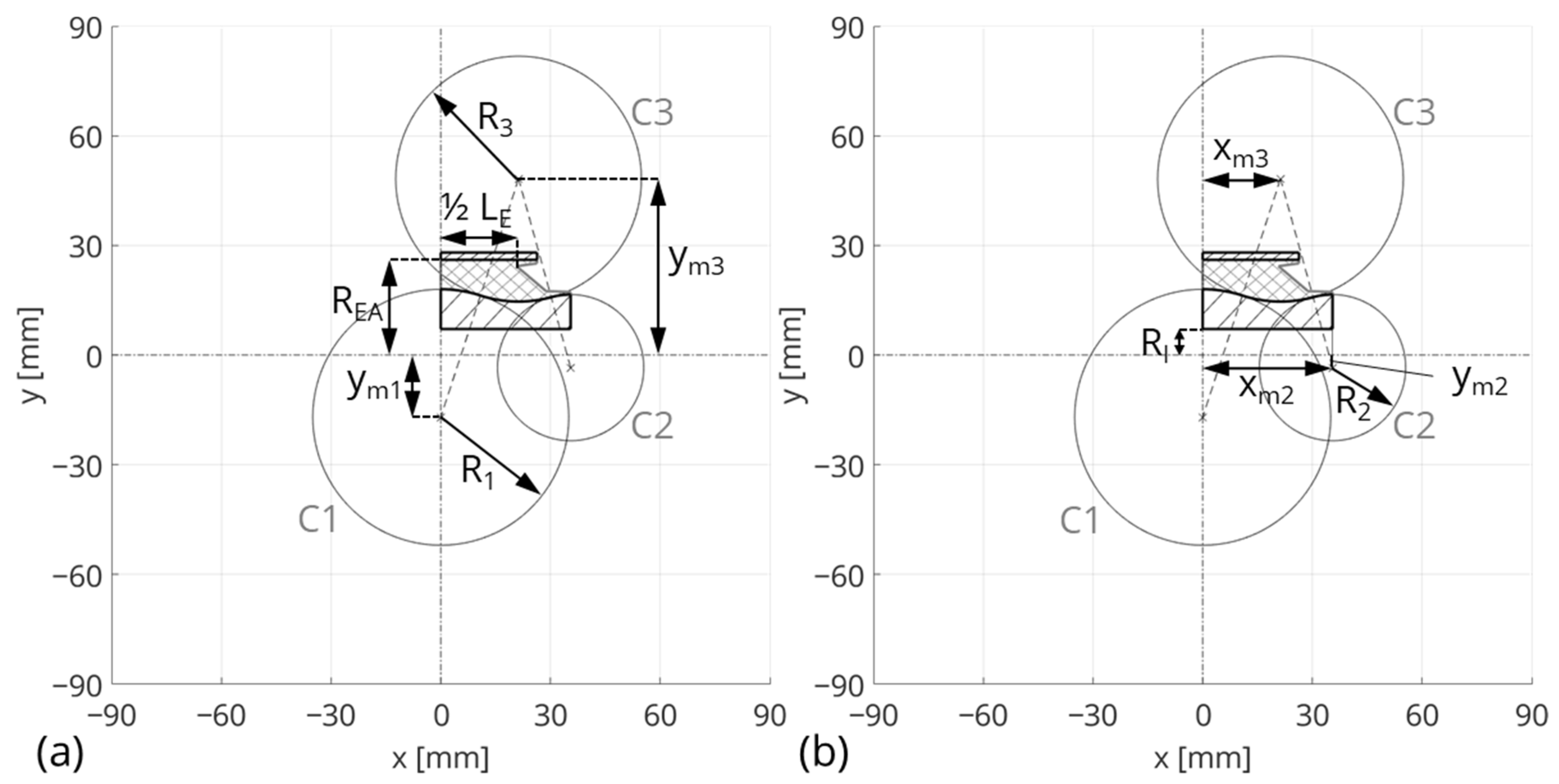
In this section, the design parameters varied in the design study are described. The geometrical modeling of the reference bushing is shown in Figure 6. Figure 6a shows the six varying design parameters using the LHS. Figure 6b represents parameters that are fixed or defined as a function of other parameters.

Using the symmetry properties of the bushing, the geometrical modeling can be described by one quarter of the bushing, as shown in Figure 6. The geometrical model definition of the inner core is based on the three circles C1, C2, and C3. Each of the circles is defined by the three parameters $x_m$, $y_m$, and $R$. The design study includes the parameters $R_1$, $y_{m1}$, $R_3$, and $y_{m3}$ of the inner core; the parameter $L_E$, which defines the width of the elastomer in the x-direction; and the parameter $R_{EA}$, which defines the outer radius of the elastomer in the y-direction (see Figure 6a).

The circle C1 is defined in the x-direction with $x_{m1}=0$ in the middle of the bushing. The radius of circle 2 is defined with a fixed value of $R_2=20\mathrm{m}\mathrm{m}$. At the inner core, there is a hole with $R_I=7.1\mathrm{m}\mathrm{m}$. The parameter $x_{m2}$ depends on $L_E$ and represents the half-length of the inner core (see Figure 6b). Due to the model simplification of the free elastomer contour, the parameter $f$ is added to the width of the elastomer:

$$x_{m2}=f+\frac{1}{2}{L}_E.$$

(8)

The parameters $x_{m3}$ and $y_{m2}$ are defined by

$$x_{m3}=\sqrt{{\left(R_1+R_3\right)}^2-{\left(\left|y_{m1}\right|+\left|y_{m3}\right|\right)}^2},$$

(9)

$$y_{m2}=y_{m3}-\sqrt{{\left(R_2+R_3\right)}^2-{\left(x_{m2}-x_{m3}\right)}^2}.$$

(10)

4.4. Constraints of the Geometrical Model

The geometrical model definition of the contour of the inner core requires that C3 is tangentially touched by C1 and C2. This leads to constraints, which restrict the design parameter space. The first constraint results from the requirement $x_{m3}>0$ and is defined by

$$R_3+R_1>\left|y_{m3}\right|+\left|y_{m1}\right|.$$

(11)

The requirement of a positive gradient of the connecting line between the two circle centers C1 and C3 leads to a further constraint

$$y_{m1}<y_{m3}.$$

(12)

Ensuring a negative gradient of the connecting line between the two circle centers C3 and C2, a constraint is given by

$$x_{m2}>x_{m3}.$$

(13)

A further constraint results from the requirement of the negative gradient regarding the connecting line between the two circle centers C3 and C2. The requirement $y_{m3}>y_{m2}$ leads to

$$R_2+R_3>x_{m2}-x_{m3}.$$

(14)

Ensuring a realistic bushing design requires additional constraints that further restrict the design parameter space. The first requirement concerns the elastomer layer thickness in the y-direction, which should be fulfilled over the entire width in the x-direction. For this purpose, a minimum and a maximum elastomer layer thickness, $T_{E,min}$ and $T_{E,max}$, as well as the following three constraints, are defined

$$R_1-\left|y_{m1}\right|<R_{EA}-T_{E,min},$$

(15)

$$R_1-\left|y_{m1}\right|>R_{EA}-T_{E,max},$$

(16)

$$R_2-\left|y_{m2}\right|<R_{EA}-T_{E,min}.$$

(17)

Another requirement is based on the material thickness of the inner core. The parameter $T_M$ and the following three constraints represent this requirement

$$R_1-\left|y_{m1}\right|>R_I+T_M,$$

(18)

$$\left|y_{m3}\right|-R_3>R_I+T_M,$$

(19)

$$R_2-\left|y_{m2}\right|>R_I+T_M.$$

(20)

The inner core of the reference bushing is coated with a thin elastomer layer over the full length of the bushing. Due to this, a last constraint is defined, which requires a minimum elastomer layer thickness between the corner point at angle $\gamma$ and the contour of the inner core. This corner point is described with the coordinates $A_x$ and $A_y$.

$$A_x=x_{m2}-e,$$

(21)

$$A_y=R_2+y_{m2}+d+\left(e·\mathit{tan}\left(\delta -90°\right)\right).$$

(22)

The description of the contour of the inner core at position $x=A_x$ is given by the equation of the circle C3.

$${R_3}^2={\left(A_x-x_{m3}\right)}^2+{\left(y_{C3}-y_{m3}\right)}^2.$$

(23)

Rearranging Equation (22) yields for the lower part of circle C3

$$y_{C3}=y_{m3}-\sqrt{{R_3}^2-{\left(A_x-x_{m3}\right)}^2}.$$

(24)

Consequently, the last constraint is defined with the aid of parameter $T_{E,A}$.

$$A_y>y_{C3}+T_{E,A}.$$

(25)

The fixed parameters of the constraints for the design study are illustrated in

Table 6. Fixed parameters of the constraints for the design study.

${\mathit{T}}_{\mathit{E},\mathit{m}\mathit{i}\mathit{n}}$ (mm)	${\mathit{T}}_{\mathit{E},\mathit{m}\mathit{a}\mathit{x}}$ (mm)	${\mathit{T}}_{\mathit{M}}$ (mm)	${\mathit{T}}_{\mathit{E},\mathit{A}}$ (mm)
3.5	8	5	1

.

4.5. Data Generation

The design parameter space used for the design study is defined in

Table 7. Design parameter space used for the design study.

	${\mathit{R}}_1$ (mm)	${\mathit{R}}_3$ (mm)	$\frac{1}{2}{\mathit{L}}_{\mathit{E}}$ (mm)	${\mathit{y}}_{\mathit{m}1}$ (mm)	${\mathit{y}}_{\mathit{m}3}$ (mm)	${\mathit{R}}_{\mathit{E}\mathit{A}}$ (mm)
min	30	30	12	−20	45	20.5
max	40	40	18	−15	50	24.45

. The number of initial samples is $n_r=\mathrm{20,000}$. With the constraints, the design parameter space is cleaned and $n_{r,valid}=2322$ valid samples remain.

Based on this cleaned design parameter space, the database for the training of the ANNs is generated. The simulation campaign required for this is automated using a Matlab-based workflow.

5. Machine-Learning-Based Surrogate Model

5.1. Fundamentals of Neural Networks

In the context of machine learning, ANNs are trained using data and a computer algorithm learns correlations inside the data [27]. The structure of an ANN is inspired by the biological nervous system and consists of neurons arranged in several layers [28]. The neurons are always connected to all neurons of the next layer and process information. The topology of a typical ANN is shown schematically in Figure 7.

The first layer is called the input layer and represents the input data. Next is the hidden layer, which consists of neurons and enables the internal processing of the input data of the network. Finally, the output layer represents the processed data in the defined dimension of the output vector. A classical form of a feed-forward neural network (FFNN) with a multilayer architecture is also called a multilayer perceptron (MLP). The number of neurons in each layer and the number of hidden layers represent hyper-parameters of the neural network and influence the performance and prediction accuracy. Following [29], the information processing between two layers is described by

$$h_j=f_a\left({\sum }_{i=1}^D{W}_{ji}^{\left(M\right)}·x_i^{\left(M\right)}+w_{j0}\right).$$

(26)

The matrix $W_{ji}^M$ represents the weights and the vector $w_{j0}$ represents the bias of each layer. The dimension of the input signal $x_i$ is defined as $i$. The output is described by the vector $h_j$ and occurs in the subsequent layer, which is denoted by superscript $M$ and defined by the number of output nodes with dimension $j$. In the case of the first layer, the global input $x$ corresponds to input vector $x_i^M$. The input vector of the subsequent layer corresponds to the output vector of the previous layer. An activation function of the layer is denoted by $f_a$ and can be considered as a further hyper-parameter. The most commonly used activation functions are tangent hyperbolic $\tanh \left(x\right)$, linear activation function, sigmoid function $\sigma \left(x\right)={\left[1+\mathrm{e}\mathrm{x}\mathrm{p}\left(-x\right)\right]}^{-1}$, and the rectifier activation function $\mathrm{R}\mathrm{e}\mathrm{L}\mathrm{U}\left(x\right)=\mathrm{m}\mathrm{a}\mathrm{x}\left(0,x\right)$. A more detailed description of the activation functions can be found in [28].

5.2. Training of the Neural Network

To adapt the ANN to a certain task, the adaptation of the network parameters (weights and biases) is called training. The training of the ANN is, in general, a mathematical optimization procedure that minimizes the approximation error between the prediction and the true value by adjusting the network parameters.

In this work, a loss function based on the mean squared error (MSE) is used to describe the minimization problem

$$\mathcal{L}\left(\upsilon \right)={\mathcal{L}}_{\mathrm{M}\mathrm{S}\mathrm{E}}\left(y^{\mathrm{t}\mathrm{r}\mathrm{u}\mathrm{e}}\left(x\right),y^{\mathrm{p}\mathrm{r}\mathrm{e}\mathrm{d}}\left(x,\upsilon \right)\right)=\frac{1}{N_{\mathrm{d}\mathrm{a}\mathrm{t}\mathrm{a}}}{\sum }_{i=1}^{N_{\mathrm{d}\mathrm{a}\mathrm{t}\mathrm{a}}}{‖y_i^{\mathrm{t}\mathrm{r}\mathrm{u}\mathrm{e}}\left(x_i\right)-y_i^{\mathrm{p}\mathrm{r}\mathrm{e}\mathrm{d}}\left(x_i,\upsilon \right)‖}^2.$$

(27)

The weights $W$ and bias $w_{j0}$ are summarized in the vector $\upsilon \in {\mathbb{R}}^{n_p}$, where $n_p$ denotes the total number of network parameters. The ground truth $y^{\mathrm{t}\mathrm{r}\mathrm{u}\mathrm{e}}\left(x\right)$ is defined as a number $N_{\mathrm{d}\mathrm{a}\mathrm{t}\mathrm{a}}$ of input–output pairs of the underlying problem. The prediction from the ANN is denoted by ${\mathrm{y}}^{pred}\left(\mathrm{x},\mathsf{\upsilon }\right)$. The minimization of the loss function is defined as

$${\upsilon }^{\star }=\arg \underset{\upsilon \in {\mathbb{R}}^{n_p}}{\min }\mathcal{L}\left(\upsilon \right),$$

(28)

where ${\upsilon }^{\star }$ represents the optimal set of hyper-parameters.

In this work, the optimization algorithm according to Kingma and Ba [30], called the Adam optimizer, is used. The algorithm is based on the gradient descent method, in which the network parameters are updated in each iteration, called an epoch:

$${\upsilon }^{k+1}={\upsilon }^k-\check{\eta }\frac{1}{N_{\mathrm{d}\mathrm{a}\mathrm{t}\mathrm{a}}}{\sum }_{i=1}^{N_{\mathrm{d}\mathrm{a}\mathrm{t}\mathrm{a}}}\frac{\partial L\left(y_i^{\mathrm{t}\mathrm{r}\mathrm{u}\mathrm{e}}\left(x_i\right),y_i^{\mathrm{p}\mathrm{r}\mathrm{e}\mathrm{d}}\left(x,{\upsilon }^k\right)\right)}{\partial {\upsilon }^k}.$$

(29)

The hyper-parameter $\check{\eta }$ defines the size of the update step and is called the learning rate. The data volume of the total training data is defined by $N_{\mathrm{d}\mathrm{a}\mathrm{t}\mathrm{a}}$.

5.3. Setup of the Neural Network Used in This Study

In this work, the ANN learns the relationships between the design parameters and the stiffnesses. For each stiffness, a separate MLP model is created and the input values of each MLP model correspond to the six design parameters of the design study, shown in Table 7. The output values represent the three scalar stiffnesses. To increase the performance of the learning process and the prediction accuracy of the ANN, the input and output values are presented in normalized form. The MLP models are implemented using TensorFlow and KerasTuner. A schematic illustration of the neural-network model used is shown in Figure 8.

In this work, 80% of the database (ground truth, consisting of $n_{r,valid}=2322$ input–output pairs) is used for the training processes and 20% of the database ($n_{r,test}=464$) is used to evaluate the accuracies of the ANN models. The number of epochs, where the network parameters are updated, is set to 5000. To regularize the training process (avoidance of under- or overfitting), the regularization strategies of early stopping and dropout are used, see [31] and [27], respectively. The dropout is controlled by a hyper-parameter $d_r$, called the dropout rate.

5.4. Hyper-Parameter Optimization

In the context of machine learning, parameters that control the setup and behavior of the learning algorithm are called hyper-parameters. These parameters have a major influence on the prediction quality of the ANN and the performance of the learning process. The optimal setup of hyper-parameters is determined using a hyper-parameter optimization based on Bayesian optimization. For that, a surrogate for the objective is built, and the uncertainty in that surrogate is quantified using Gaussian process regression. From this surrogate objective, an acquisition function is defined to determine the next sampling points. A detailed description is given in [32]. A brief overview of further approaches for hyper-parameter optimization as well as another technique based on deep reinforcement learning can be found in [33]. The optimization process uses as an objective function the validation loss based on the test dataset. The value ranges of the hyper-parameters are summarized in

Table 8. Value ranges of the hyper-parameter optimization.

Hyper-Parameter	Description	Options
${\mathit{N}}_{\mathit{H}\mathit{L}}$	number of hidden layers	$N_{HL}=\left[1:1:10\right]$
${\mathit{N}}_{\mathit{N}}$	number of neurons per layer	$N_N=\left[8:4:128\right]$
${\mathit{d}}_{\mathit{r}}$	dropout rate	$d_r=\left[0:0.005:0.02\right]$
${\mathit{f}}_{\mathit{a}}$	activation function	$f_a=\left\{\mathrm{l}\mathrm{i}\mathrm{n}\mathrm{e}\mathrm{a}\mathrm{r},\mathrm{s}\mathrm{i}\mathrm{g}\mathrm{m}\mathrm{o}\mathrm{i}\mathrm{d},\mathrm{R}\mathrm{e}\mathrm{L}\mathrm{U},\mathrm{t}\mathrm{a}\mathrm{n}\mathrm{h}\right\}$
$\check{\mathit{\eta }}$	learning rate	$\check{\eta }=\left\{0.01,0.001,0.0001\right\}$

.

The results of the best training configurations after the Bayesian optimization are shown in

Table 9. Architecture of the MLP models for the radial, axial, and torsional stiffnesses.

Hyper-Parameter	${\mathit{c}}_{\mathit{r}\mathit{a}\mathit{d}}$	${\mathit{c}}_{\mathit{a}\mathit{x}}$	${\mathit{c}}_{\mathit{t}\mathit{o}\mathit{r}\mathit{s}}$
${\mathit{N}}_{\mathit{H}\mathit{L}}$	8	8	10
${\mathit{N}}_{\mathit{N}}$	8 in each hidden layer	{104, 16, 20, 116, 100, 32, 56, 8}	{128, 96, 8, 8, 12, 80, 60, 8, 8, 8}
${\mathit{d}}_{\mathit{r}}$	0 in each hidden layer	0.005 in each hidden layer	0 in each hidden layer
${\mathit{f}}_{\mathit{a}}$	ReLU in each hidden layer	{tanh, tanh, ReLU, tanh, σ, σ, tanh, ReLU}	{ReLU, ReLU, tanh, ReLU, ReLU, σ, ReLU, ReLU, ReLU, ReLU}
$\check{\mathit{\eta }}$	0.01	0.001	0.001

.

The evaluation of the accuracies of each ANN model is based on the MAPE according to the following equation with $dir=\left\{rad,ax,tors\right\}$.

$$\mathrm{M}\mathrm{A}\mathrm{P}\mathrm{E}=f_{\mathrm{M}\mathrm{A}\mathrm{P}\mathrm{E}}\left(c^{\mathrm{t}\mathrm{r}\mathrm{u}\mathrm{e}},c^{\mathrm{p}\mathrm{r}\mathrm{e}\mathrm{d}}\right)=\frac{1}{n_{r,test}}{\sum }_{i=1}^{n_{r,test}}\left|\frac{c_{dir,i}^{\mathrm{t}\mathrm{r}\mathrm{u}\mathrm{e}}-c_{dir,i}^{\mathrm{p}\mathrm{r}\mathrm{e}\mathrm{d}}}{c_{dir,i}^{\mathrm{t}\mathrm{r}\mathrm{u}\mathrm{e}}}\right|.$$

(30)

The upper half of Figure 9 illustrates the true and predicted stiffnesses of the three loading directions; the lower half shows the corresponding relative prediction errors.

The ANN model of the radial stiffness has the highest total prediction error with $\mathrm{M}\mathrm{A}\mathrm{P}\mathrm{E}=2.46\%$. This is also shown in the level of the relative prediction errors in Figure 9, bottom left. In ranges of small stiffness values, the highest relative errors are present. The axial stiffness has smaller relative prediction errors (see Figure 9, bottom middle) and a smaller total prediction error with $\mathrm{M}\mathrm{A}\mathrm{P}\mathrm{E}=0.55\%$. The total prediction error of the ANN model for torsional stiffness is the smallest over the entire test dataset, with $\mathrm{M}\mathrm{A}\mathrm{P}\mathrm{E}=0.3\%$, and the ANN model has the smallest relative prediction errors (see Figure 9, bottom right).

Table 10. Prediction accuracies of the ANN models for the radial, axial, and torsional stiffnesses.

	${\mathit{c}}_{\mathit{r}\mathit{a}\mathit{d}}$	${\mathit{c}}_{\mathit{a}\mathit{x}}$	${\mathit{c}}_{\mathit{t}\mathit{o}\mathit{r}\mathit{s}}$
MAPE (%)	2.46	0.55	0.3

shows the accuracies of the ANN models.

6. Design Optimization

6.1. Methodology and Problem Description

The trained ANN models in Section 5 predict stiffnesses (target values) based on the input of geometrical parameters (design parameters) of a bushing. For the use of these ANN models in the vehicle development process, especially in early development phases, it is necessary to invert this design process as described in this section. This results in an inverse mathematical problem and is solved in this work by optimizing the design parameters to achieve the required stiffnesses under given geometrical constraints. The resulting design optimization is realized using PSO. Analogously to the procedure presented in Section 3, the optimization problem is described by minimizing the MAPE. The required stiffnesses are given by $c^{\mathrm{r}\mathrm{e}\mathrm{q}}$ and the predicted stiffnesses from the ANN models are defined by $c^{\mathrm{p}\mathrm{r}\mathrm{e}\mathrm{d}}$.

During the optimization, invalid design parameter combinations can occur due to the geometrically invalid domains in the design parameter space. Consequently, the PSO algorithm must be extended. The basis for this extension is the degree of fulfillment of a particle with regard to its constraints (see Equations (11)–(20) and (25)). Based on a rating term $r_n$, according to Röber [34], a rating is assigned to each particle $n\in S$, which contains the information on whether a particle is valid or not, and how far away this particle is from the valid domain.

$$r_n=r_{max}·\left(r_n^C-\frac{1}{1+‖r_n^v‖}\right).$$

(31)

In the first step, for each constraint that is not fulfilled, the absolute distance to fulfill the constraint is determined by a calculation of the residuum and saved in the vector $r_n^v$. If all constraints are fulfilled, the value 0 is assigned to $r_n^v$ for this particle. In the next step, the rank $r_n^C$ is calculated for each particle, where the number of failed constraints is defined as $N_{fc}$.

$$r_n^C=1+N_{fc}.$$

(32)

Finally, the maximum rank of one particle of all iterations thus far is stored in $r_n^{max}$. Consequently, the information of the ranks of the particles (degree of fulfillment with respect to the constraints of each particle) is used in the objective function ${\mathcal{L}}_{\mathrm{D}\mathrm{O}}$. The design parameters are summarized in the vector $x_{\mathrm{D}\mathrm{P}}\in {\mathbb{R}}^{n_{\mathrm{D}\mathrm{P}}}$, where $n_{\mathrm{D}\mathrm{P}}$ denotes the number of design parameters. The objective function ${\mathcal{L}}_{\mathrm{D}\mathrm{O}}$ is defined as

$$\begin{array}{ll}{\mathcal{L}}_{\mathrm{D}\mathrm{O}}\left(x_{\mathrm{D}\mathrm{P}}\right)=& \frac{1}{3}\left(\left|\frac{c_{rad}^{\mathrm{r}\mathrm{e}\mathrm{q}}-c_{rad}^{\mathrm{p}\mathrm{r}\mathrm{e}\mathrm{d}}\left(x_{\mathrm{D}\mathrm{P}}\right)}{c_{rad}^{\mathrm{r}\mathrm{e}\mathrm{q}}}\right|+\left|\frac{c_{ax}^{\mathrm{r}\mathrm{e}\mathrm{q}}-c_{ax}^{\mathrm{p}\mathrm{r}\mathrm{e}\mathrm{d}}\left(x_{\mathrm{D}\mathrm{P}}\right)}{c_{ax}^{\mathrm{r}\mathrm{e}\mathrm{q}}}\right|+\left|\frac{c_{tors}^{\mathrm{r}\mathrm{e}\mathrm{q}}-c_{tors}^{\mathrm{p}\mathrm{r}\mathrm{e}\mathrm{d}}\left(x_{\mathrm{D}\mathrm{P}}\right)}{c_{tors}^{\mathrm{r}\mathrm{e}\mathrm{q}}}\right|\right)\\ & +\left(r_n^C-\frac{1}{1+‖r_n^v‖}\right)·r_n^{max}.\end{array}$$

(33)

Finally, the mathematical constraint optimization problem can be formulated as

$$x_{\mathrm{D}\mathrm{P}}^{\star }=\arg \underset{x\in {\mathbb{R}}^{n_{\mathrm{DP}}}}{\min }{\mathcal{L}}_{\mathrm{D}\mathrm{O}}\left(x_{\mathrm{D}\mathrm{P}}\right)$$

(34)

$$\mathrm{s}\mathrm{u}\mathrm{b}\mathrm{j}\mathrm{e}\mathrm{c}\mathrm{t} \mathrm{t}\mathrm{o} \mathrm{g}\mathrm{e}\mathrm{o}\mathrm{m}\mathrm{e}\mathrm{t}\mathrm{r}\mathrm{i}\mathrm{c}\mathrm{a}\mathrm{l} \mathrm{c}\mathrm{o}\mathrm{n}\mathrm{s}\mathrm{t}\mathrm{r}\mathrm{a}\mathrm{i}\mathrm{n}\mathrm{t}\mathrm{s} \mathrm{E}\mathrm{q}\mathrm{u}\mathrm{a}\mathrm{t}\mathrm{i}\mathrm{o}\mathrm{n}\mathrm{s} \left(11\right)–\left(20\right) \mathrm{a}\mathrm{n}\mathrm{d} \left(25\right),$$

where $x_{\mathrm{D}\mathrm{P}}^{\star }$ represents the optimal set of design parameters. In the initialization of the PSO algorithm, $n$ particles are randomly drawn. This leads to the fact that invalid particles also exist at the beginning. To increase the performance of the PSO algorithm, a loop is implemented to ensure that only valid particles are generated after the initialization.

6.2. Numerical Examples

In this study, two typical usecases are defined to demonstrate the usability of the design optimization algorithm based on the ANN models in the bushing development process. In the first usecase, the quasi-static stiffnesses are required in the radial, axial, and torsional load directions. In addition to the target values, the second usecase requires that the outer dimensions of the bushing be smaller than a certain value due to installation space requirements. Accordingly, the design optimization algorithm must determine the optimal set of design parameters for the bushing to fulfill the requirements in both cases. The described usecases are shown in

Table 11. Requirements of the two usecases.

	${\mathit{c}}_{\mathit{r}\mathit{a}\mathit{d}}^{\mathbf{r}\mathbf{e}\mathbf{q}}$ (kN/mm)	${\mathit{c}}_{\mathit{a}\mathit{x}}^{\mathbf{r}\mathbf{e}\mathbf{q}}$ (kN/mm)	${\mathit{c}}_{\mathit{t}\mathit{o}\mathit{r}\mathit{s}}^{\mathbf{r}\mathbf{e}\mathbf{q}}$ (Nm/°)	$\frac{1}{2}{\mathit{L}}_{\mathit{E}}$ (mm)	${\mathit{R}}_{\mathit{E}\mathit{A}}$ (mm)
Usecase 1	8	0.6	3.5	-	-
Usecase 2	10	0.7	4	≤13	≤21

.

For both usecases, the number $n$ of particles per iteration $t$ is defined as 60. To reduce the simulation effort, the number of iterations of both usecases is set to 20.

6.3. Results of the Design Optimization

Table 12. Results of the first usecase.

	${\mathit{c}}_{\mathit{r}\mathit{a}\mathit{d}}$ (kN/mm)	${\mathit{c}}_{\mathit{a}\mathit{x}}$ (kN/mm)	${\mathit{c}}_{\mathit{t}\mathit{o}\mathit{r}\mathit{s}}$ (Nm/°)
Requirement	8	0.6	3.5
Results DO	7.9301	0.6447	3.5004
Results FEM	7.7025	0.6477	3.5039

shows the results of the first usecase from the design parameter optimization (DO) and from the final FEM simulation. The resulting stiffnesses of the DO are based on the predictions of the ANN models. Using the corresponding design parameters, an FEM model is generated and a simulation is performed to verify the ANN prediction for the found solution. Subsequently, these simulation results are used to validate the ANN models.

The minimum $\mathrm{M}\mathrm{A}\mathrm{P}\mathrm{E}$ found in the entire design optimization process is $2.78\%$ and fulfills all constraints. The related design parameters are shown in

Table 13. Design parameters of the first usecase as a result of the optimization task.

DP	${\mathit{R}}_1$ (mm)	${\mathit{R}}_3$ (mm)	$\frac{1}{2}{\mathit{L}}_{\mathit{E}}$ (mm)	${\mathit{y}}_{\mathit{m}1}$ (mm)	${\mathit{y}}_{\mathit{m}3}$ (mm)	${\mathit{R}}_{\mathit{E}\mathit{A}}$ (mm)
[lower, upper] bounds	[30, 40]	[30, 40]	[12, 18]	[−20, −15]	[45, 50]	[20.5, 24.45]
	34.4504	32.7475	12.5964	−17.7151	47.9825	21.7282

.

Table 14. Optimization task of the second usecase.

	${\mathit{c}}_{\mathit{r}\mathit{a}\mathit{d}}$ (kN/mm)	${\mathit{c}}_{\mathit{a}\mathit{x}}$ (kN/mm)	${\mathit{c}}_{\mathit{t}\mathit{o}\mathit{r}\mathit{s}}$ (Nm/°)	$\frac{1}{2}{\mathit{L}}_{\mathit{E}}$ (mm)	${\mathit{R}}_{\mathit{E}\mathit{A}}$ (mm)
Requirement	10	0.7	4	≤13	≤21
Results DO	10.006	0.7416	3.9968	12.552	20.9137
Results FEM	10.2002	0.7491	4.007	-	-

presents the second usecase. As shown in Table 12, the resulting stiffnesses of the DO are based on the predictions of the ANN models and a finite element model is generated with the corresponding design parameters. The simulation is conducted and the ANN models are validated with the simulation results.

The minimum $\mathrm{M}\mathrm{A}\mathrm{P}\mathrm{E}$ found in the entire design optimization process is $2.03\%$ and fulfills all constraints. The related design parameters are shown in

Table 15. Design parameters of the second usecase as a result of the optimization task.

DP	${\mathit{R}}_1$ (mm)	${\mathit{R}}_3$ (mm)	$\frac{1}{2}{\mathit{L}}_{\mathit{E}}$ (mm)	${\mathit{y}}_{\mathit{m}1}$ (mm)	${\mathit{y}}_{\mathit{m}3}$ (mm)	${\mathit{R}}_{\mathit{E}\mathit{A}}$ (mm)
[lower, upper] bounds	[30, 40]	[30, 40]	[12, 13]	[−20, −15]	[45, 50]	[20.5, 21]
	35.421	33.6226	12.552	−18.2982	47.3173	20.9137

.

Table 16. Prediction errors of the usecases.

	MAPE (%) (Requirement-DO)	MAPE (%) (DO-FEM)	MAPE (%) (Requirement-FEM)
Usecase 1	2.78	1.15	3.93
Usecase 2	2.03	1.07	3.06

summarizes the prediction errors based on the MAPE of the two usecases between the target values (requirement), the results of the DO, and the results of the bushing designs simulated with ABAQUS (FEM).

For both usecases, the prediction error between the target values and the stiffnesses from the DO is less than 3%. The prediction error between the DO and the FEM simulation is less than 2% in both cases and, consequently, smaller than the prediction error between the target values and the DO. This indicates a very good prediction accuracy of the ANN models. The slightly greater uncertainty is in the optimization algorithm. For both cases, the accuracy between the required target values and the simulated stiffnesses based on the design parameters from the DO is less than 4%. Due to the small prediction errors, a very good design accuracy of the entire method is shown.

To evaluate the performance of the rating term (see Equation (31)), the number of valid particles in all iterations is considered in Figure 10.

The initialization of the PSO algorithm is completed at iteration 0. As mentioned, this results in 60 valid particles. In the first iteration, the lowest number of valid particles is present. Due to the rating of the invalid particles in the objective function, the number of valid particles increases again. At iteration 4, a plateau near the maximum number of defined particles of the PSO algorithm is reached. Generally, this behavior is present in both usecases. The second usecase has a marginally smaller number of valid particles over all iterations. This can be explained by the additional geometrical restrictions in comparison to usecase 1, which results in a more complex optimization task for the PSO algorithm. Finally, it can be said that the use of the rating method based on the rating term (Equations (31) and (34)) is well suited to the DO with constraints in this study.

7. Conclusions

In this work, the application of ANNs was investigated for the design process of chassis bushings. The nonlinear and strongly geometry-dependent transfer behavior resulting from the elastomer of the bushing was modeled by ANNs.

In the first step, a physical chassis bushing was characterized on a multi-axial elastomer test rig. Subsequently, a reference bushing based on the physical bushing was created as a finite element model in the simulation environment ABAQUS. The geometrical modeling of the inner core and outer sleeve was approximated with basic geometrical elements and relations between them. The free elastomer contour required an optical measurement and was modeled as a spline. To model the material behavior, the material model according to Yeoh was used. The material parameters for the Yeoh model were determined using a subsequent material parameter optimization based on PSO and the measurement results of the physical bushing. For the subsequent design study, a geometrical model simplification was conducted regarding the optically measured elastomer contour. Subsequently, the geometrical model simplification was validated in relation to the reference bushing model. The resulting FEM model represented the simplified bushing model for the design study.

In the next step, six design parameters were defined for the geometrical design of the bushing, which represented the basis for the subsequent design study. Based on the DoE method of Latin hypercube sampling, 20,000 samples were created in a design parameter space to generate the training data. To avoid invalid geometrical models within the design parameter space, geometrical constraints were defined. Subsequently, the design parameter space was cleaned, resulting in 2322 valid samples.

In the following step, the cleaned design parameter space formed the basis for the training of the ANNs. For the stiffness prediction in the radial, axial, and torsional load directions, one ANN was trained each. The network training was based on the Adam optimizer and 80% of the data was used for the training process. The remaining 20% of the data was used for the validation of the trained networks. To increase the prediction accuracy of the ANN, a hyper-parameter optimization based on Bayesian optimization was performed, resulting in three different ANN topologies.

Finally, a DO was presented using the ANN for the design process. The basis for this was PSO which was extended to address the geometrical constraints. To showcase the performance of the DO, two usecase studies were discussed and the accuracy of the DO was evaluated. In the first usecase, target values in the form of quasi-static stiffnesses of the radial, axial, and torsional load directions were required. In the second usecase, in addition to the required target values of the quasi-static stiffnesses, two installation space requirements (width and outer diameter of the elastomer body) were defined. Using DO, the optimal design parameters to fulfill the target values were determined in each case. In both cases, a MAPE < 3% was achieved between the target values and the stiffnesses from the DO. To evaluate the deviation between the ANN prediction and the results of the FEM simulation using the resulting design parameters from the DO, the MAPE was calculated. In both usecases, the MAPE was smaller than 2%.

The small prediction errors represent a very good prediction accuracy of the ANN models as well as good design accuracy of the entire method. In future work, the transferability of the method to other types of chassis bushings (e.g., bushings with an intermediate sleeve) should be tested. Furthermore, the method can also be generalized and used for installation space issues with other components. In addition, the extension to more complex optimization tasks, including multi-objective optimization, should be investigated.

References

- Huber, W. Industrie 4.0 in der Automobilproduktion; Springer Fachmedien: Wiesbaden, Germany, 2016. [Google Scholar] [CrossRef]
- Winkelhake, U. Die Digitale Transformation der Automobilindustrie, 2nd ed.; Springer: Berlin/Heidelberg, Germany, 2021. [Google Scholar] [CrossRef]
- Klostermeier, R.; Haag, S.; Benlian, A. Digitale Zwillinge—Eine explorative Fallstudie zur Untersuchung von Geschäftsmodellen. HMD Prax. Wirtsch. 2018, 55, 297–311. [Google Scholar] [CrossRef]
- Ersoy, M.; Gies, S. Fahrwerkhandbuch, 5th ed.; Springer Fachmedien: Wiesbaden, Germany, 2017. [Google Scholar] [CrossRef]
- Adkins, J.E.; Gent, A.N. Load-deflexion relations of rubber bush mountings. Br. J. Appl. Phys. 1954, 5, 354–358. [Google Scholar] [CrossRef]
- Göbel, E.F. Gummifedern; Springer: Berlin/Heidelberg, Germany, 1969. [Google Scholar] [CrossRef]
- Töpel, E.; Büttner, K.; Penisson, C.; Prokop, G. Discussion of Static Calculation Methods for Chassis Bushings. In Proceedings of the 28th Aachen Colloquium Automobile and Engine Technology 2019, Aachen, Germany, 7–9 October 2019; Eckstein, L., Pischinger, S., Eds.; pp. 1661–1674. [Google Scholar]
- TrelleborgVibracoustic. Schwingungstechnik im Automobil: Grundlagen Werkstoffe Konstruktion Berechnung und Anwendungen, 1st ed.; Vogel Business Media: Würzburg, Germany, 2015. [Google Scholar]
- Stommel, M.; Stojek, M.; Korte, W. FEM zur Berechnung von Kunststoff- und Elastomerbauteilen, 2nd ed.; Hanser: München, Germany, 2018. [Google Scholar] [CrossRef]
- Liu, C.-H.; Hsu, Y.-Y.; Yang, S.-H. Geometry Optimization for a Rubber Mount with Desired Stiffness Values in Two Loading Directions Considering Hyperelasticity and Viscoelasticity. Int. J. Automot. Technol. 2021, 22, 609–619. [Google Scholar] [CrossRef]
- Kaya, N.; Erkek, M.Y.; Güven, C. Hyperelastic modelling and shape optimisation of vehicle rubber bushings. Int. J. Veh. Des. 2016, 71, 212–225. [Google Scholar] [CrossRef]
- Jung, Y.-W.; Kim, H.-K. Prediction of Nonlinear Stiffness of Automotive Bushings by Artificial Neural Network Models Trained by Data from Finite Element Analysis. Int. J. Automot. Technol. 2020, 21, 1539–1551. [Google Scholar] [CrossRef]
- Cernuda, C.; Llavori, I.; Zavoianu, A.-C.; Aguirre, A.; Zabala, A.; Plaza, J. Critical Analysis of the Suitability of Surrogate Models for Finite Element Method Application in Catalog-Based Suspension Bushing Design. In Proceedings of the 2020 25th IEEE International Conference on Emerging Technologies and Factory Automation (ETFA), Vienna, Austria, 8–11 September 2020; IEEE: Piscataway, NJ, USA, 2020; pp. 829–836. [Google Scholar]
- Ernst, S.; Thüringer, T.; Töpel, E.; Büttner, K.; Prokop, G. Multiaxial characterisation and modelling of complex elastomeric mount properties for determining virtual spectrum load data. Int. J. Fatigue 2021, 150, 106312. [Google Scholar] [CrossRef]
- Uriarte, I.; Zulueta, E.; Guraya, T.; Arsuaga, M.; Garitaonandia, I.; Arriaga, A. Characterization of recycled rubber using particle swarm optimization techniques. Rubber Chem. Technol. 2015, 88, 343–358. [Google Scholar] [CrossRef]
- Rivlin, R.S.; Saunders, D.W. Large elastic deformations of isotropic materials, V.I.I. Experiments on the deformation of rubber” Philosophical Transactions of the Royal Society of London. Ser. A Math. Phys. Sci. 1951, 243, 251–288. [Google Scholar]
- Balke, H. Einführung in Die Technische Mechanik, 3rd ed.; Springer: Berlin/Heidelberg, Germany, 2014. [Google Scholar] [CrossRef]
- Yeoh, O.H. Some Forms of the Strain Energy Function for Rubber. Rubber Chem. Technol. 1993, 66, 754–771. [Google Scholar] [CrossRef]
- Systèmes, D. ABAQUS 6.14 Getting Started with Abaqus: Interactive Edition; Dassault Systèmes Simulia Corp.: Providence, RI, USA, 2014. [Google Scholar]
- Lee, K.; Park, J. Application of Particle Swarm Optimization to Economic Dispatch Problem: Advantages and Disadvantages. In Proceedings of the 2006 IEEE PES Power Systems Conference and Exposition, Atlanta, GA, USA, 29 October–1 November 2006; IEEE: Piscataway, NJ, USA; pp. 188–192. [Google Scholar]
- Helwig, S. Particle Swarms for Constrained Optimization. Ph.D. Thesis, Friedrich-Alexander-Universitaet, Erlangen, Germany, 2010. [Google Scholar]
- Kennedy, J.; Eberhart, R. Particle swarm optimization. In Proceedings of the International Conference on Neural Networks, Perth, WA, Australia, 27 November–1 December 1995; IEEE: Piscataway, NJ, USA, 1995; pp. 1942–1948. [Google Scholar]
- Schmitt, B.I. Convergence Analysis for Particle Swarm Optimization; FAU University Press: Erlangen, Germany, 2015. [Google Scholar]
- Mckay, M.D.; Beckman, R.J.; Conover, W.J. A Comparison of Three Methods for Selecting Values of Input Variables in the Analysis of Output From a Computer Code. Technometrics 2000, 42, 55–61. [Google Scholar] [CrossRef]
- Siebertz, K.; van Bebber, D.; Hochkirchen, T. Statistische Versuchsplanung, 2nd ed.; Springer: Berlin/Heidelberg, Germany, 2017. [Google Scholar] [CrossRef]
- Olsson, A.; Sandberg, G.; Dahlblom, O. On Latin hypercube sampling for structural reliability analysis. Struct. Saf. 2003, 25, 47–68. [Google Scholar] [CrossRef]
- Goodfellow, I.; Courville, A.; Bengio, Y. Deep Learning; The MIT Press: Cambridge, MA, USA, 2016. [Google Scholar]
- Da Silva, I.N.; Hernane Spatti, D.; Andrade Flauzino, R.; Liboni, L.H.B.; dos Reis Alves, S.F. Artificial Neural Networks; Springer International Publishing: Cham, Germany, 2017. [Google Scholar] [CrossRef]
- Bishop, C.M. Pattern Recognition and Machine Learning, 1st ed.; Springer: New York, NY, USA, 2016. [Google Scholar]
- Kingma, D.P.; Ba, J. Adam: A Method for Stochastic Optimization. arXiv 2014, arXiv:1412.6980. [Google Scholar]
- Montavon, G.; Orr, G.B.; Müller, K.-R. Neural Networks: Tricks of the Trade, 2nd ed.; Springer: Berlin/Heidelberg, Germany, 2012. [Google Scholar] [CrossRef]
- Frazier, P.I. A Tutorial on Bayesian Optimization. arXiv 2018, arXiv:1807.02811. [Google Scholar]
- Fuchs, A.; Heider, Y.; Wang, K.; Sun, W.; Kaliske, M. DNN²: A hyper-parameter reinforcement learning game for self-design of neural network based elasto-plastic constitutive descriptions. Comput. Struct. 2021, 249, 106505. [Google Scholar] [CrossRef]
- Röber, M. Multikriterielle Optimierungsverfahren für Rechenzeitintensive Technische Aufgabenstellungen. Ph.D. Thesis, Technische Universität Chemnitz, Chemnitz, Germany, 2012. [Google Scholar]
Figure 1.
Cross-section of the reference bushing and geometrical model of the inner core.
Figure 2.
Force–displacement characteristics of the reference bushing, measured with the test rig.
Figure 3.
Example simulation results of the reference bushing, inhomogeneous von Mises stress distribution on the deformed geometry of the elastomer under (a) radial, (b) axial, and (c,d) torsional loads scaled by factor 2 for radial load and factor 4 for axial and torsional loads.
Figure 4.
Convergence behavior of the PSO algorithm for material parameter identification. The crosses represent particles. The encircled crosses show the particle with the smallest mean absolute percentage error (MAPE) in each iteration.
Figure 5.
Model simplification and parameterization of the free elastomer contour: (a) represents the reference bushing and (b) shows the simplified bushing model.
Figure 6.
Geometrical modeling of the reference bushing: (a) represents the parameters varied within the design study, and (b) shows fixed and resulting parameters from boundary conditions.
Figure 7.
Schematic illustration of a neural network consisting of an input layer with three input parameters, a hidden layer with six neurons, and an output layer with one output parameter.
Figure 8.
Schematic illustration of the neural-network architecture used.
Figure 9.
Prediction accuracies of the ANN models for the radial, axial, and torsional stiffnesses.
Figure 10.
Performance of the ranking term based on the number of valid particles of all iterations for both usecases.