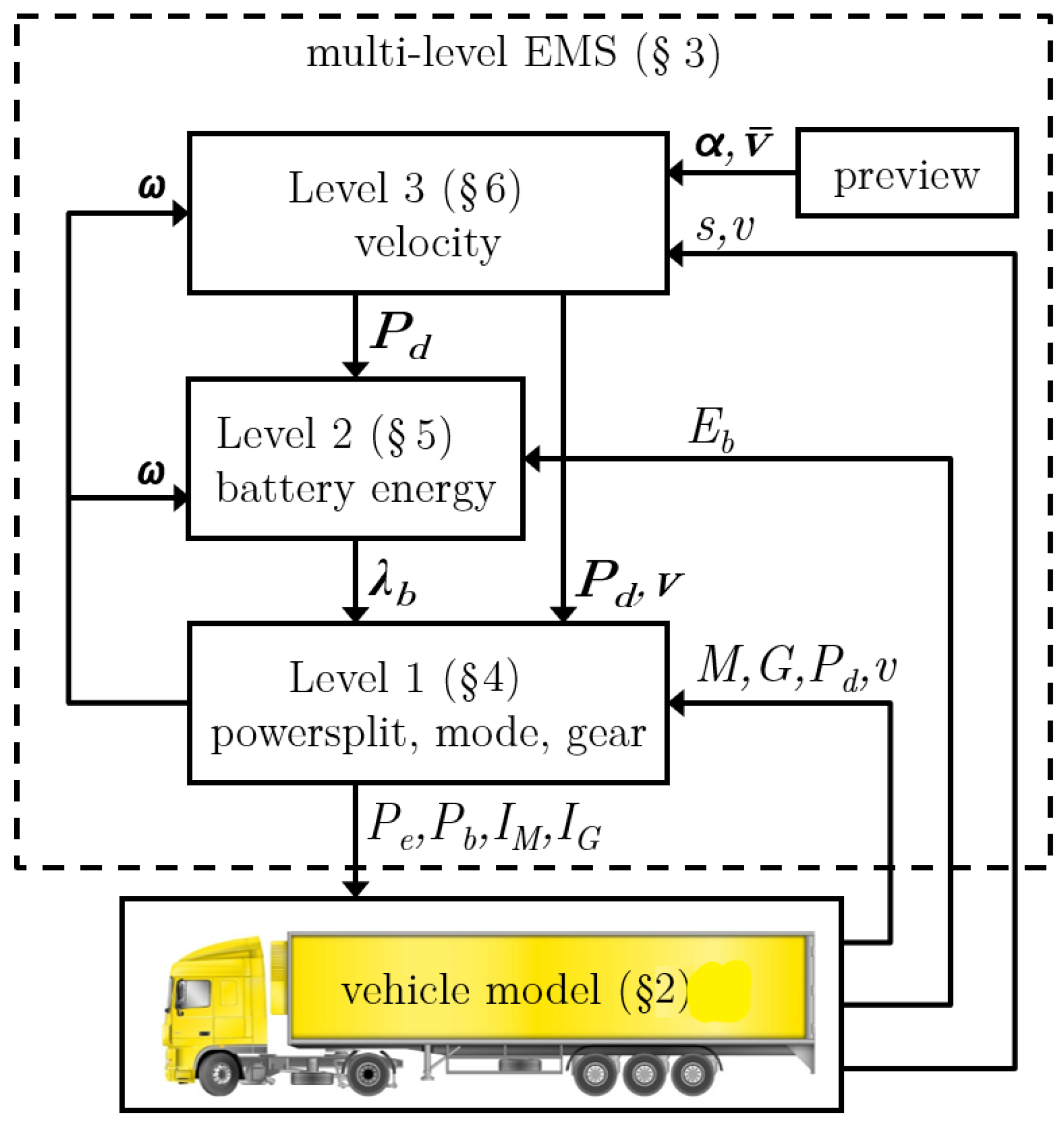
Figure 1.
Multi-level optimization of the velocity (
v), battery energy (
) and power split (
) including mode and gear selection (
). In
Section 3 the scheme is described, with the prediction of: road slope (
), velocity limit (
), driveline rotational speed (
), driveline power (
), velocity (
) and battery costate (
), dependent on: vehicle position (
s), velocity (
v), battery energy (
), driveline power (
), mode (
M) and gear (
G).
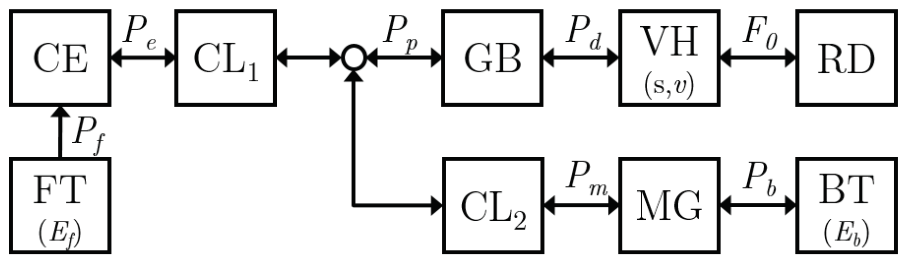
Figure 2.
Topology of the parallel Hybrid Electric Vehicle with its relevant power flows, defined positive towards the road and relevant states (between parenthesis).
Figure 2.
Topology of the parallel Hybrid Electric Vehicle with its relevant power flows, defined positive towards the road and relevant states (between parenthesis).
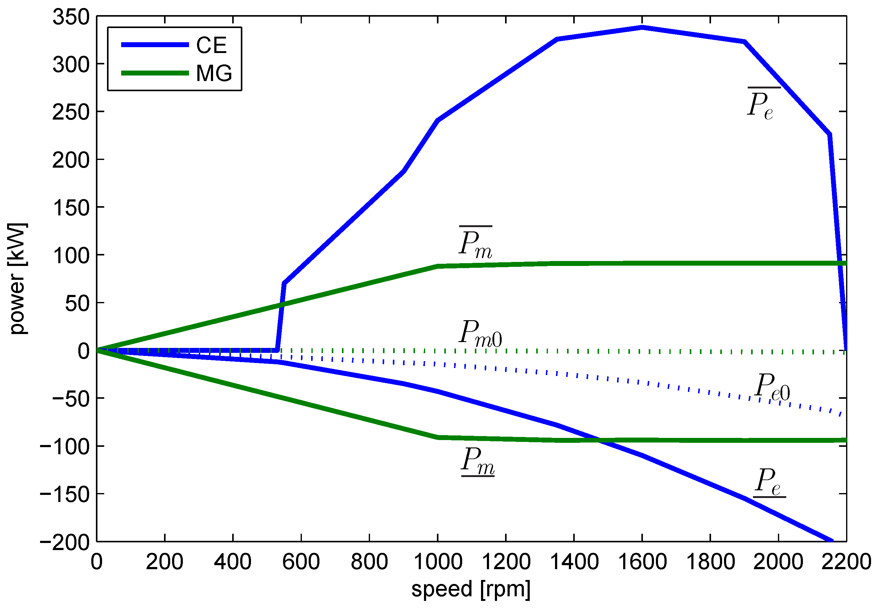
Figure 3.
Power capabilities of internal combustion engine (CE) and motor generator (MG) as a function of the rotational speed. Dotted lines indicate the nominal friction and .
Figure 3.
Power capabilities of internal combustion engine (CE) and motor generator (MG) as a function of the rotational speed. Dotted lines indicate the nominal friction and .
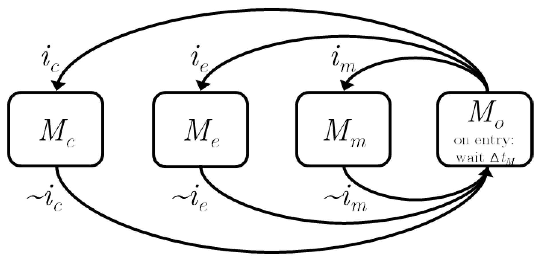
Figure 4.
State machine for switching between modes M. All mode switches go through (‘open driveline’), which is maintained for . The negation of the mode command is denoted with .
Figure 4.
State machine for switching between modes M. All mode switches go through (‘open driveline’), which is maintained for . The negation of the mode command is denoted with .
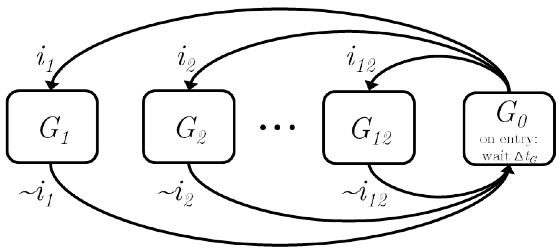
Figure 5.
State machine for switching between gears G. All gear switches go through (‘open driveline’), which is maintained for . The negation of the gear command is denoted with .
Figure 5.
State machine for switching between gears G. All gear switches go through (‘open driveline’), which is maintained for . The negation of the gear command is denoted with .
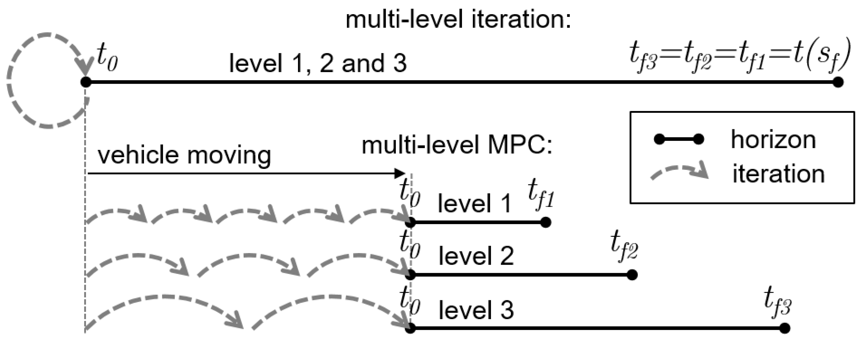
Figure 6.
Schematic of the horizon in the ‘multi-level iteration’ and ‘multi-level Model Predictive Controller (MPC)’ solution schemes. The multi-level iteration has an identical horizon, for all levels, and for all iterations, comprising the complete drive cycle. The multi-level MPC has a solution scheme, with shorter horizon lengths. With each time sample, the vehicle moves along the drive cycle. At each time sample, one iteration is performed, over a horizon starting at , having a fixed horizon length to . When the level has a faster sample time, iterations are performed more often, thereby improving the feedback performance.
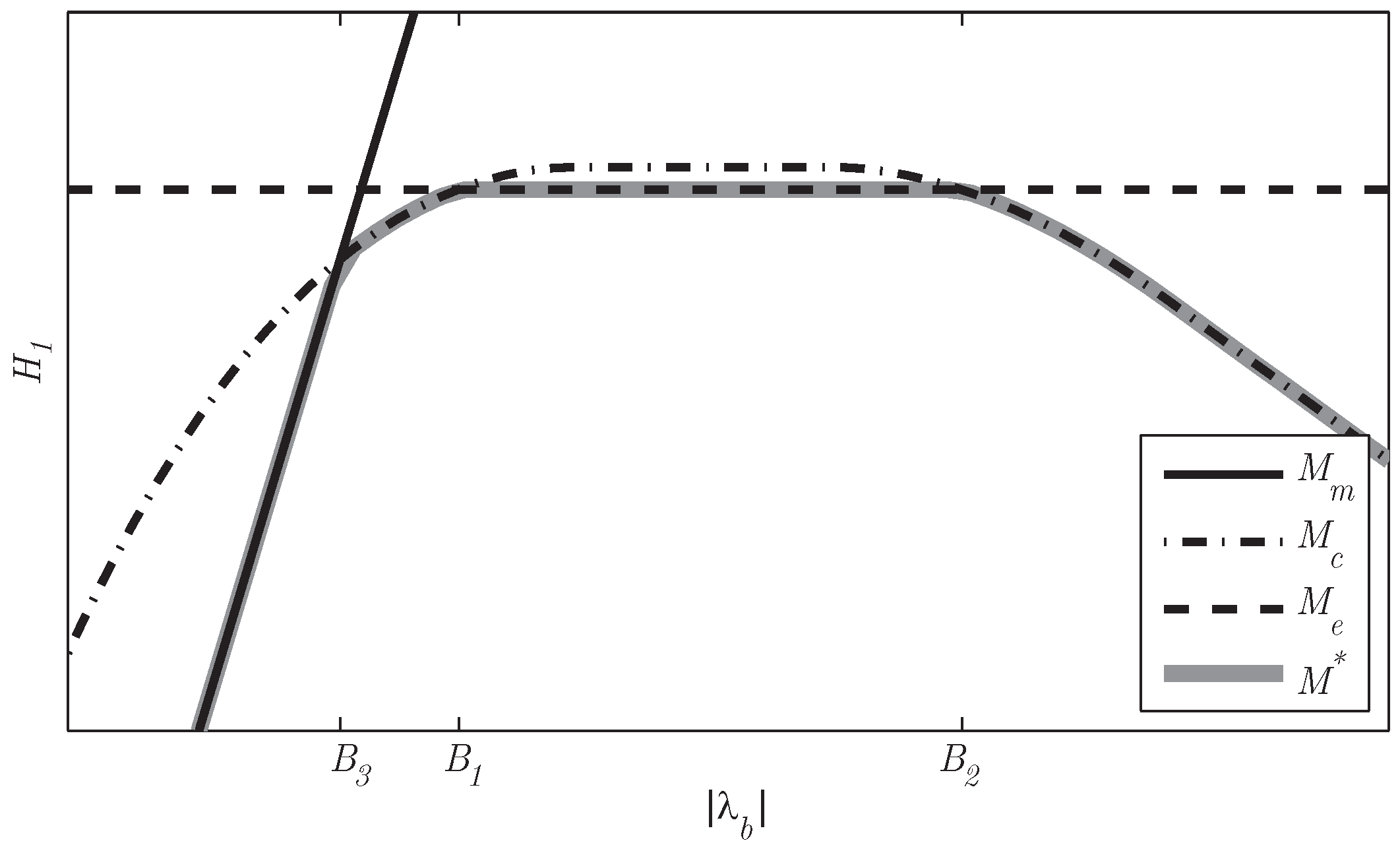
Figure 7.
The Hamiltonian of the three modes as a function of for a power demand and rotational speed. The optimal mode changes at the boundary points .
Figure 7.
The Hamiltonian of the three modes as a function of for a power demand and rotational speed. The optimal mode changes at the boundary points .
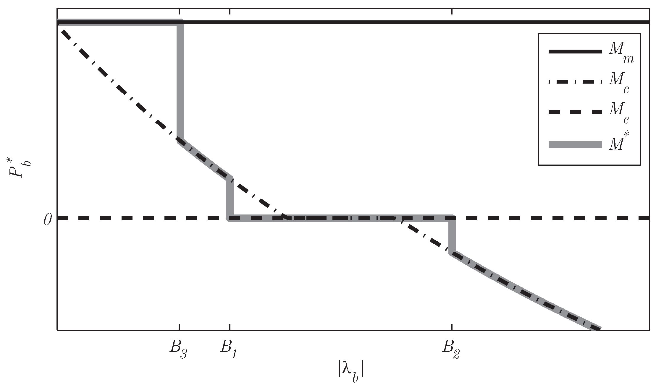
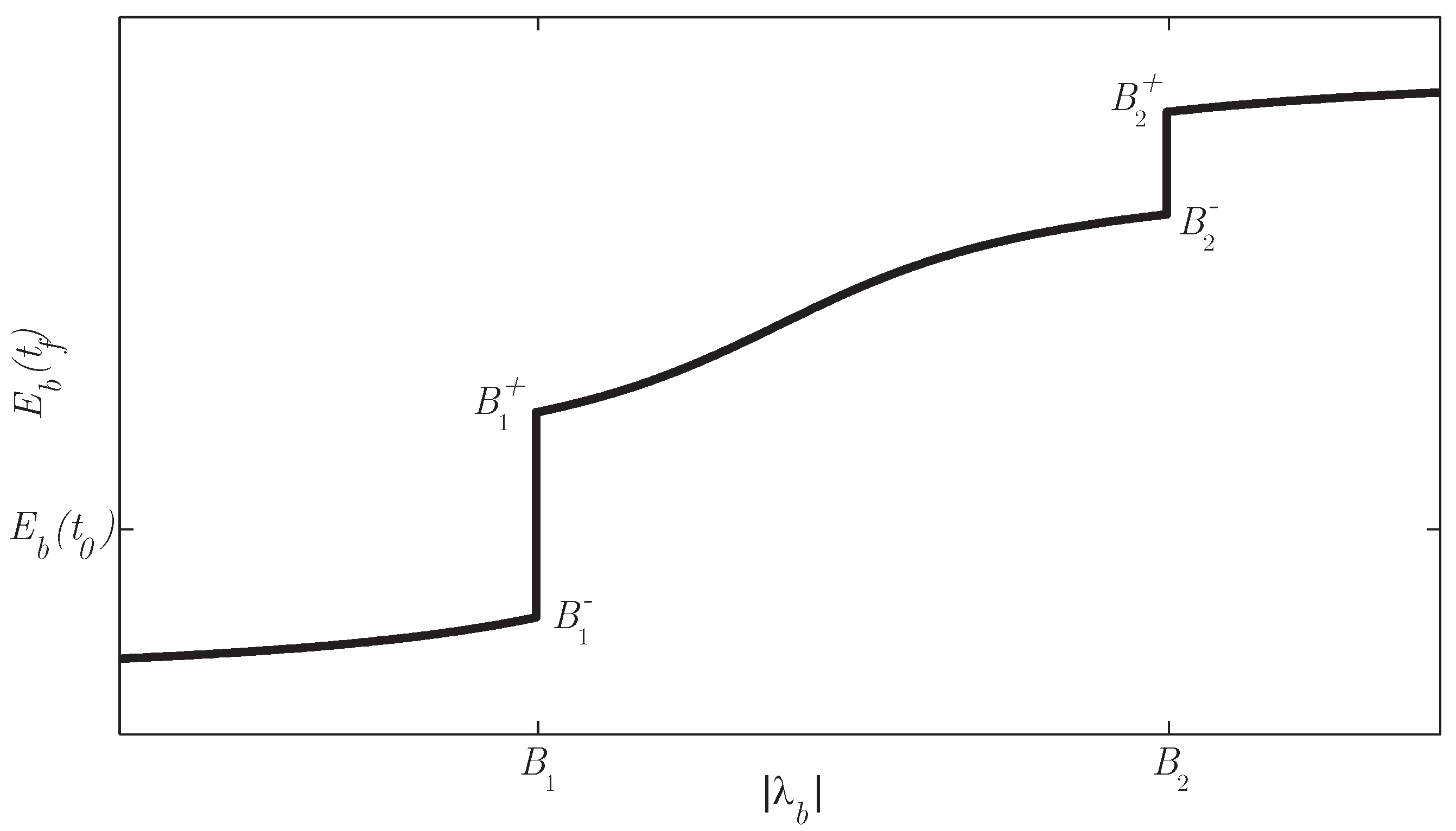
Figure 8.
as a function of for the modes for a power demand and gear. At and , the optimal mode switches between and , with a corresponding jump in . At a jump occurs due to switching between and .
Figure 8.
as a function of for the modes for a power demand and gear. At and , the optimal mode switches between and , with a corresponding jump in . At a jump occurs due to switching between and .
Figure 9.
Explicit mode change map as a function of costate
and power demand
, indicating the guards
B between the optimal modes
(motor-only),
(engine-only) and
(combined).
Figure 7 and
Figure 8 are cross sections at
.
Figure 9.
Explicit mode change map as a function of costate
and power demand
, indicating the guards
B between the optimal modes
(motor-only),
(engine-only) and
(combined).
Figure 7 and
Figure 8 are cross sections at
.
Figure 10.
Illustrating the Receding Horizon Integer Program to solve at each time step. Over a horizon of four seconds with a sampling time of one second, all feasible modes and gears are enumerated (blue), starting at the current mode and gear (red). For all feasible modes, H is calculated, increased with an equivalent fuel penalty on each mode or gear change, and the optimal trajectory over the horizon (blue dotted line) is determined, using Dynamic Programming (DP).
Figure 11.
For dealing with constraints, non-unique solutions and a limited horizon, the flowchart shows the procedure for solving the boundary value problems (BVP). Starting with one unsolved (sub)problem (SP), from to , the process is started. Dependent on the number of constraint violations, the procedure ends with a set of solved subproblems, each providing a segment of over the complete horizon. Each subproblem contains the solution to a BVP, and dependent on the stated conditions, the additional procedures I1, I2 or I3 are needed.
Figure 12.
Changing the constant for a drive cycle, causes jumps in the charge sustenance, due to non-unique (singular) solutions at and .
Figure 12.
Changing the constant for a drive cycle, causes jumps in the charge sustenance, due to non-unique (singular) solutions at and .
Figure 13.
Illustration of algorithm I2a. Power demand of a drive segment with and two optimal modes: ( is positive during high power demands, resulting in too low ) and ( is zero during high power demands, resulting in too high ). A charge sustaining trajectory (), is possible with one switch at or , or with infinitely many switchings indicated as .
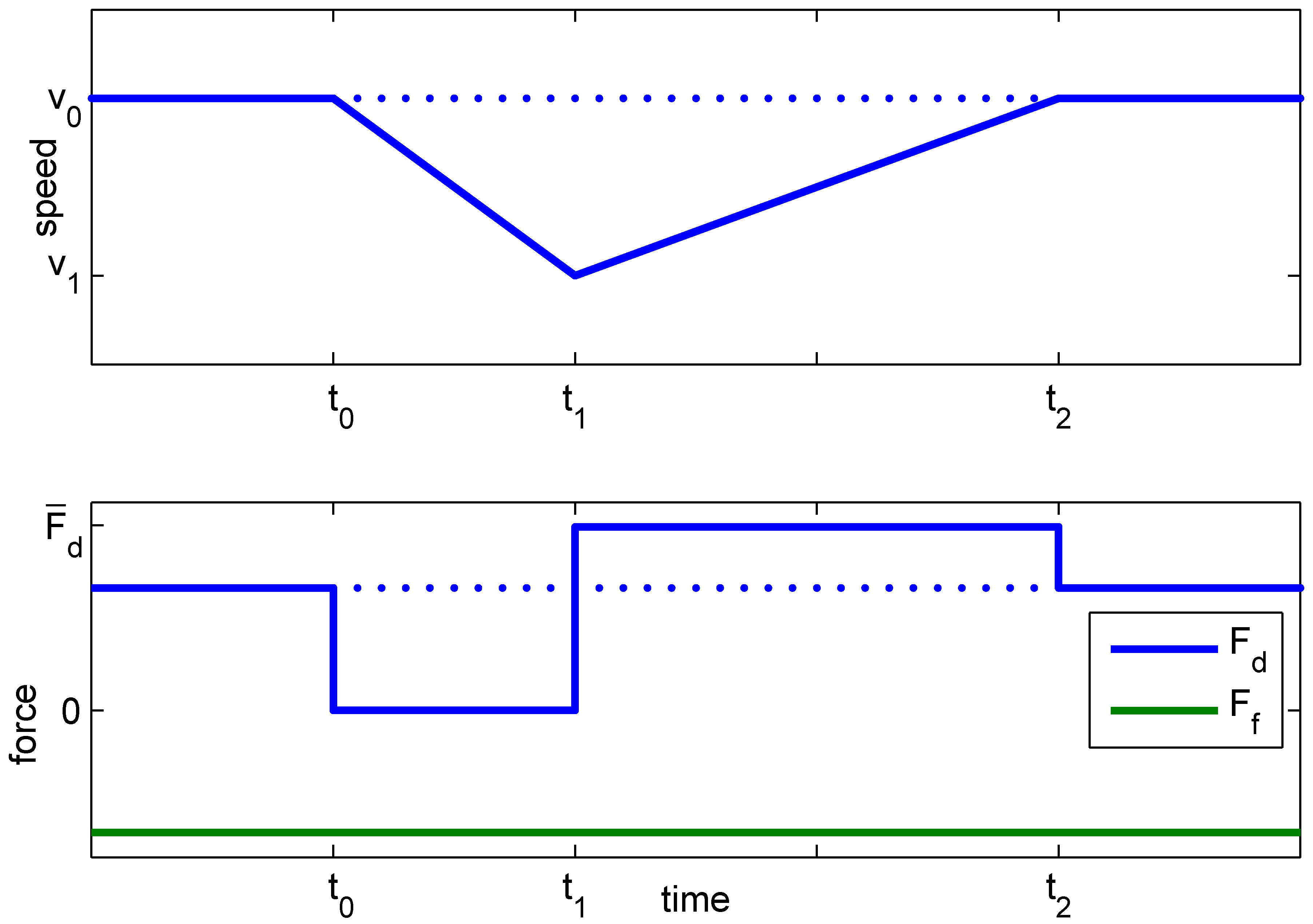
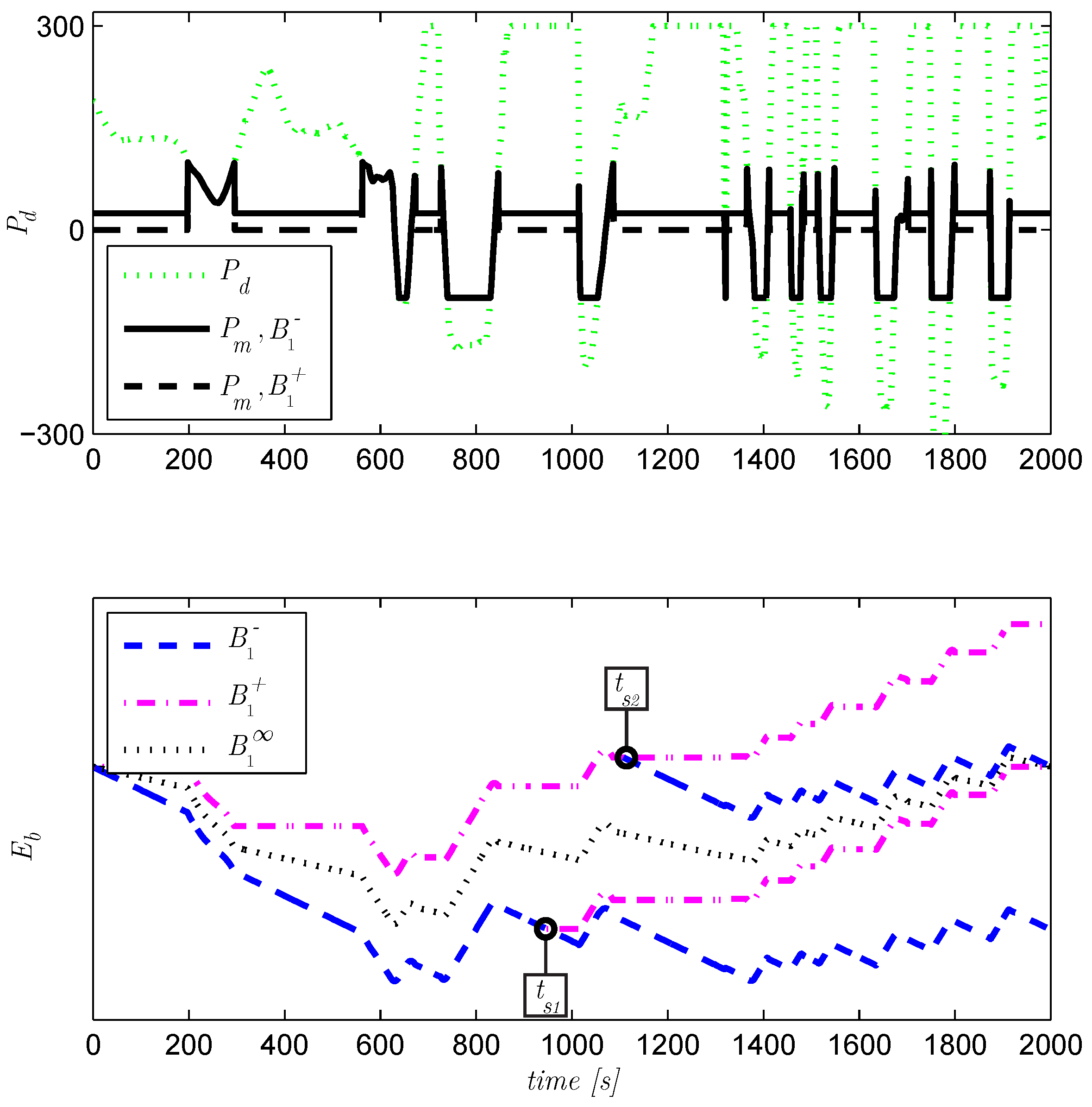
Figure 14.
Illustration of algorithm I2b, first part. Starting with the lower boundary is violated at and a switch must be made to . However, s as switching point is too late, as exceeds with .
Figure 14.
Illustration of algorithm I2b, first part. Starting with the lower boundary is violated at and a switch must be made to . However, s as switching point is too late, as exceeds with .
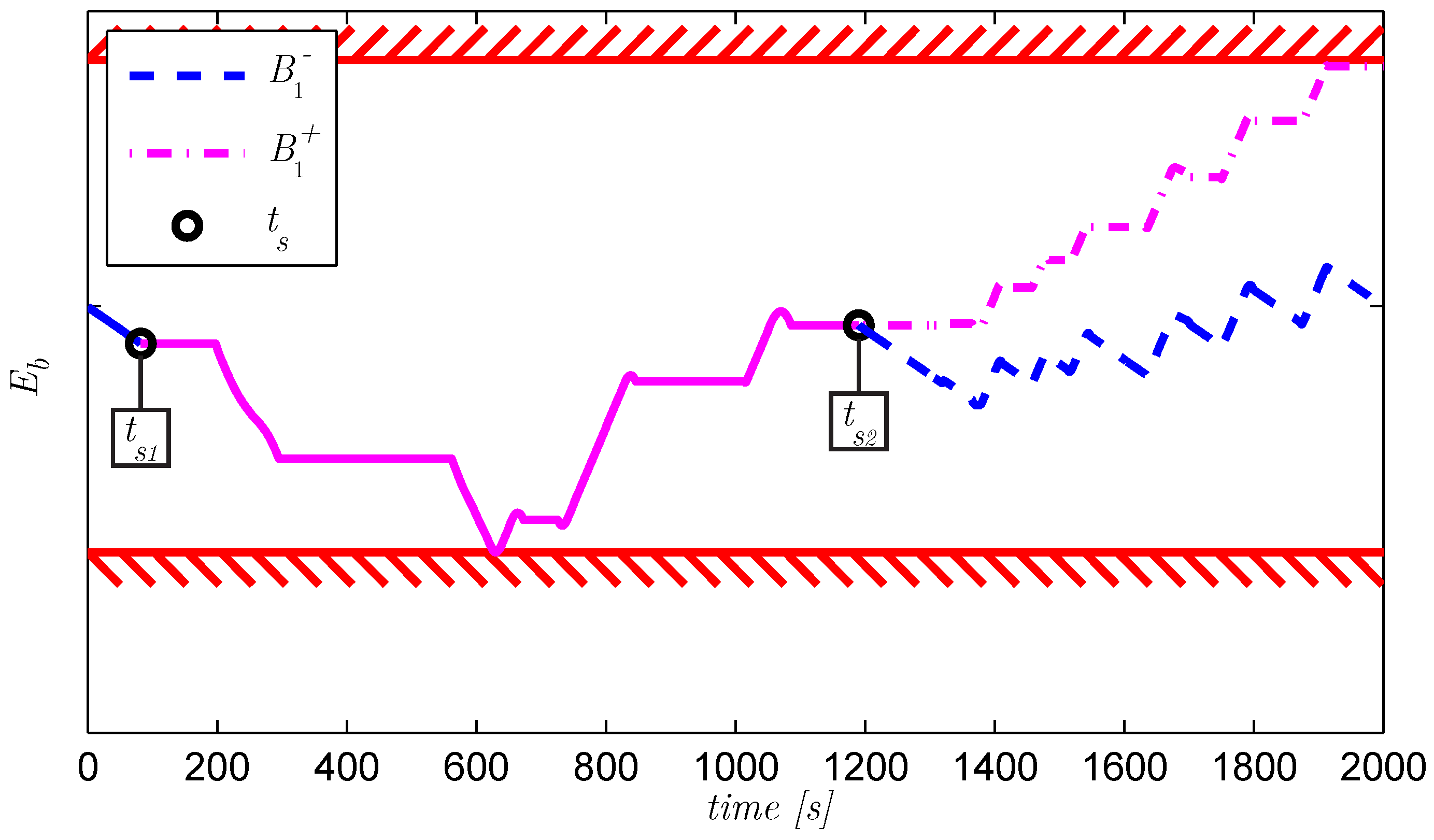
Figure 15.
Illustration of algorithm I2b, second part. A new s is found, and is continued, until at s the switch to has to be made to ensure .
Figure 15.
Illustration of algorithm I2b, second part. A new s is found, and is continued, until at s the switch to has to be made to ensure .
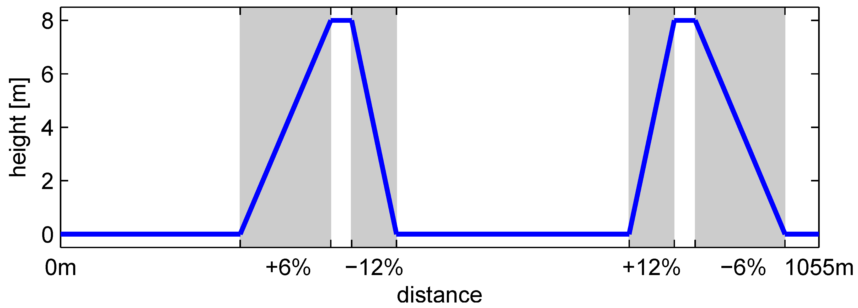
Figure 16.
Elevation profile of the short test cycle.
Figure 16.
Elevation profile of the short test cycle.
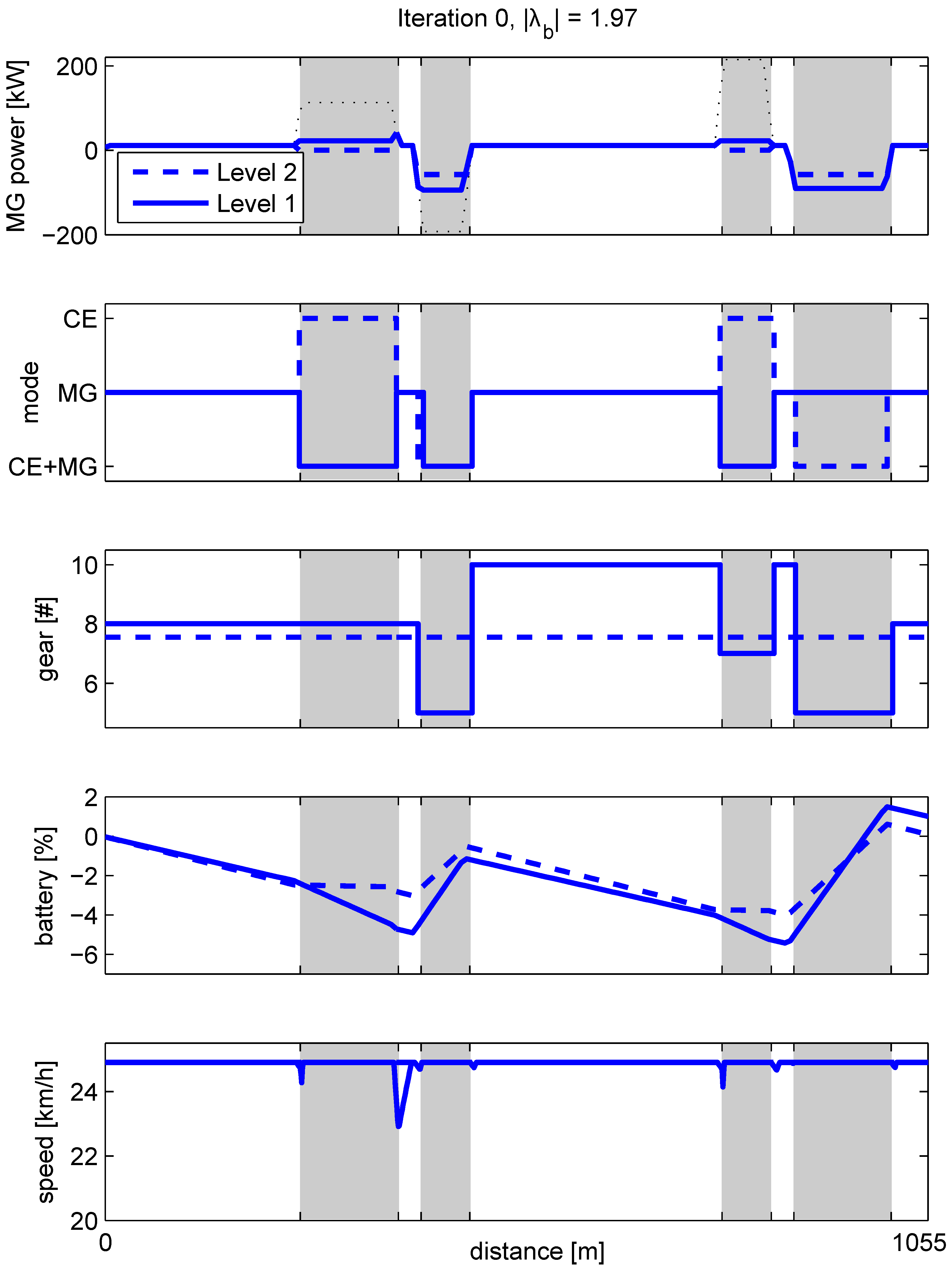
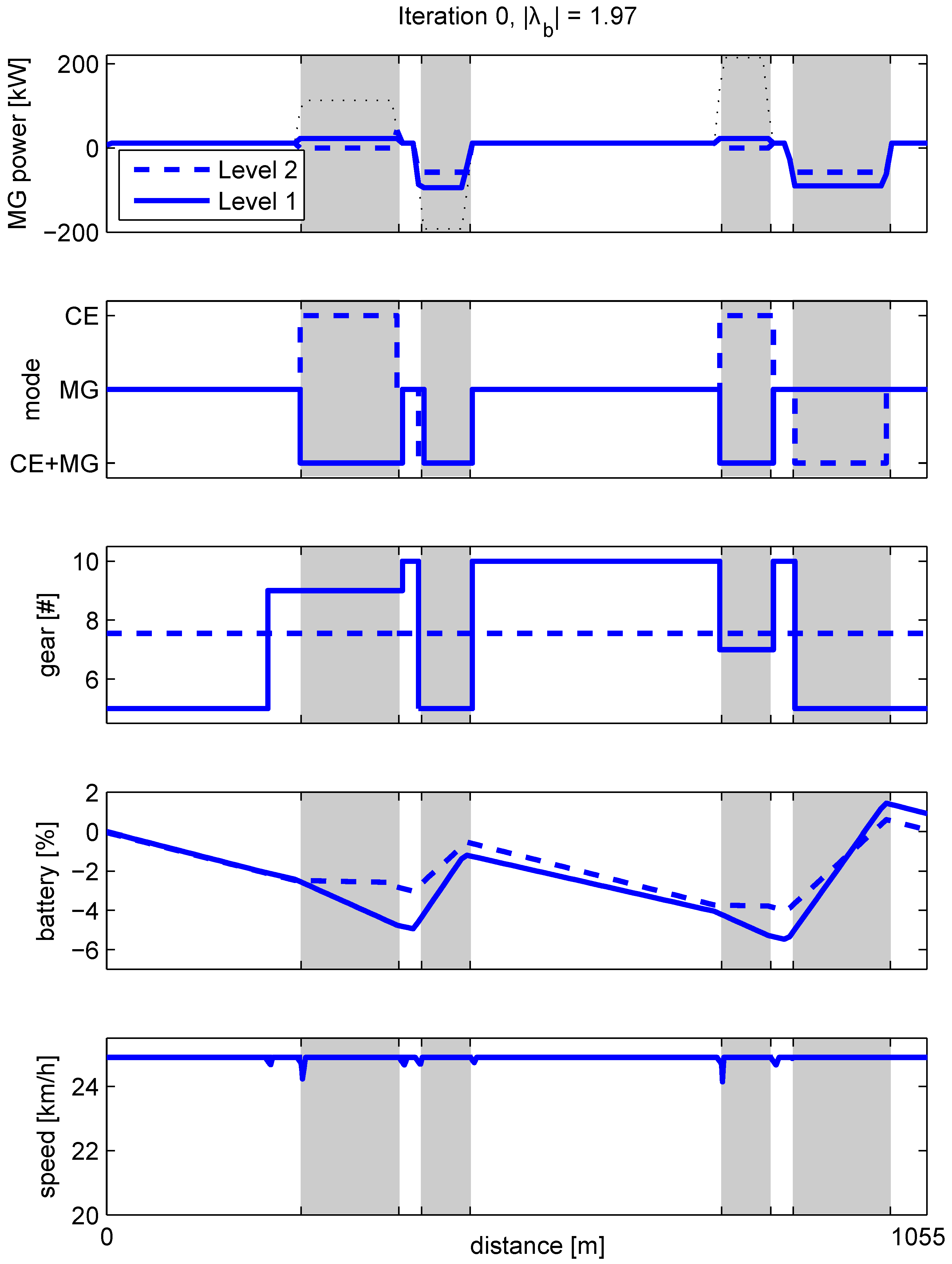
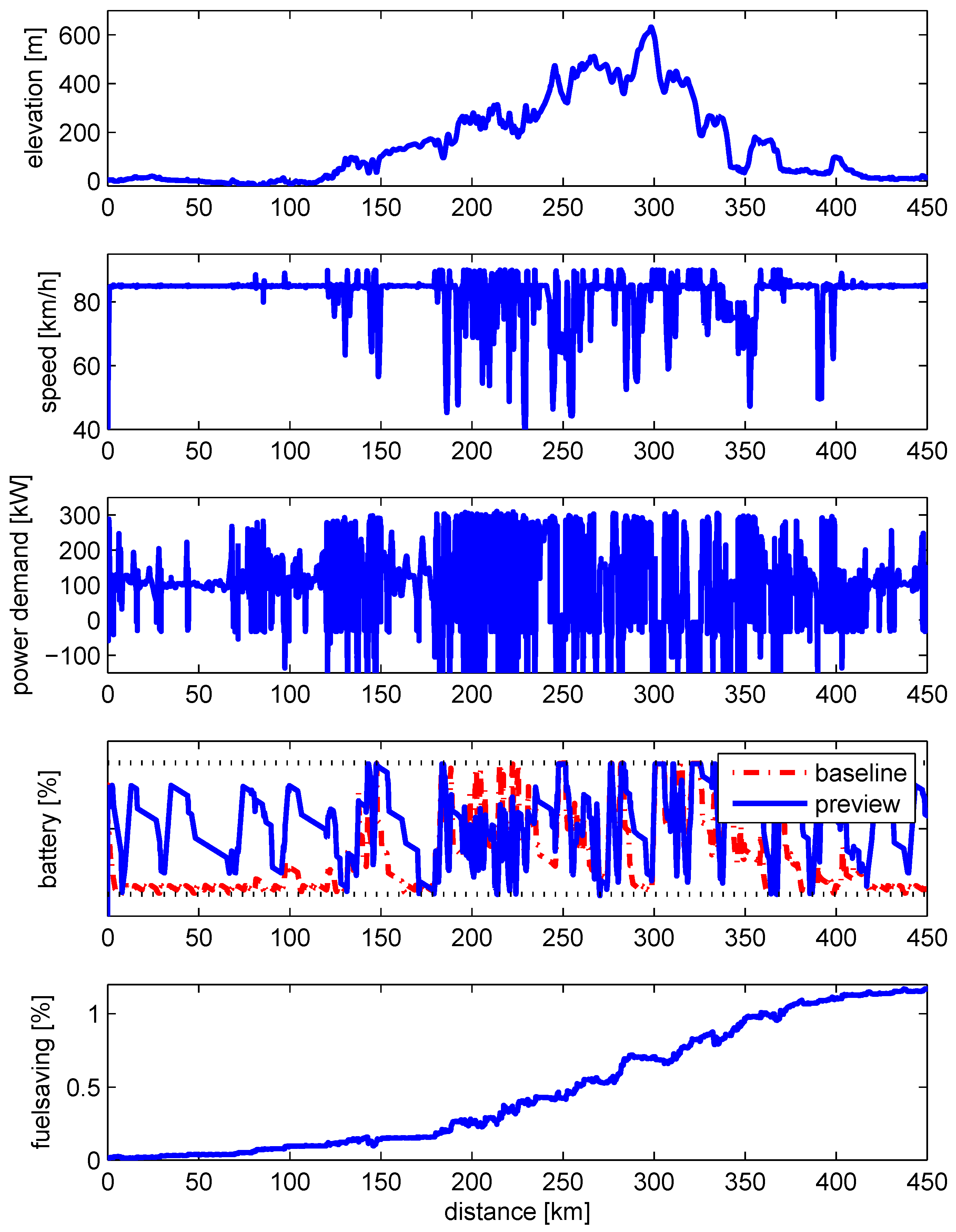
Figure 17.
High fidelity simulation results on a representative long-haul cycle. The previewing Energy Management System (EMS) saves an additional fuel to the baseline EMS.
Figure 17.
High fidelity simulation results on a representative long-haul cycle. The previewing Energy Management System (EMS) saves an additional fuel to the baseline EMS.
Table 1.
Optimizing Energy Management System (EMS) algorithms, for power-split, stop-start and gear. ‘Cost’ indicates if switching events are penalized in the algorithm. See
Table 2 for the used abbreviations.
Table 1.
Optimizing Energy Management System (EMS) algorithms, for power-split, stop-start and gear. ‘Cost’ indicates if switching events are penalized in the algorithm. See
Table 2 for the used abbreviations.
| Reference | Power-Split | Stop-Start | Gear Selection |
|---|
| [15] | PMP | PMP | - |
| [16] | QP | RB | - |
| [17] | QP | PMP | RB |
| [18] | PMP | DP | DP |
| [19] | QP | DP + cost | DP + cost |
| [20] | MILP | MILP + cost | MILP + cost |
| this work | PMP | DP + cost | DP + cost |
Table 2.
Abbreviations.
| Components |
| BT | Battery |
| CE | Combustion Engine |
| CL | Clutch |
| EMS | Energy Management System |
| FT | Fuel Tank |
| GB | Gearbox |
| HEV | Hybrid Electric Vehicle |
| MG | Motor Generator |
| RD | Road |
| VH | Vehicle |
| Algorithms |
| DP | Dynamic Program |
| MILP | Mixed Integer Linear Program |
| PMP | Pontryagin’s Minimum Principle |
| QP | Quadratic Program |
| RB | Rule Based (heuristics) |
Table 3.
Model parameters for the internal combustion engine (CE), motor generator (MG), battery (BT) and vehicle (VH).
Table 3.
Model parameters for the internal combustion engine (CE), motor generator (MG), battery (BT) and vehicle (VH).
| Model | Parameter | Value | Unit | Description |
|---|
| CE | | 0.45 | - | indicated efficiency |
| | | | W | friction (cf. Figure 3) |
| | | | W | minimum power (cf. Figure 3) |
| | | | W | maximum power (cf. Figure 3) |
| | | 3 | kg m | moment of inertia |
| MG | | 0.95 | - | mechanical efficiency |
| | | | W | friction (cf. Figure 3) |
| | | | W | minimum power (cf. Figure 3) |
| | | | W | maximum power (cf. Figure 3) |
| | | 1.5 | kg m | moment of inertia |
| BT | | | 1/W | loss coefficient |
| | | | J | effective battery size |
| VH | m | | kg | vehicle mass |
| | | 1.2 | kg/m | air density |
| | | 0.65 | - | air drag coefficient |
| | A | 10 | m | frontal area |
| | | | - | rolling resistance coefficient |
| | | 52.2 | - | drive ratio |
| | | 1.29 | - | gear base constant |
| | g | 9.8 | m/s | gravitational constant |
Table 4.
Driveline modes M.
Table 4.
Driveline modes M.
| M | Description | CL | CL | | |
|---|
| combined | closed | closed | = = | |
| engine-only | closed | open | = = 0 | |
| motor-only | open | closed | = = 0 | |
| open driveline | open | open | = = 0 | 0 |
Table 5.
Generic optimization problem, subdivided into three levels (i).
Table 5.
Generic optimization problem, subdivided into three levels (i).
| | ‘Generic’ | ‘Velocity’ | ‘Battery Energy’ | ‘Power-Split’ |
|---|
| | 3 | 2 | 1 |
| | | | |
| | | | |
| | | | |
| | 0 | 0 | |
| | | | 0 |
| | | | |
| | | | |
| | | | |
Table 6.
Explicit solution of the power-split as a function of the mode.
Table 6.
Explicit solution of the power-split as a function of the mode.
| Mode | Description | |
|---|
| motor-only | |
| engine-only | 0 |
| combined | |
Table 7.
Energy consumption over the short test cycle. MPC: model predictive controller.
Table 7.
Energy consumption over the short test cycle. MPC: model predictive controller.
| | J [MJ] | Energy Reduction [%] |
|---|
| non-hybrid | 16.8 | 0 |
| iteration 0 | 7.91 | 52.9 |
| iteration 1 | 7.90 | 53.0 |
| MPC | 7.93 | 52.8 |
Table 8.
Fuel savings on a typical long-haul route. EMS: energy management system.
Table 8.
Fuel savings on a typical long-haul route. EMS: energy management system.
| Vehicle | Fuel [l/100 km] | Fuel [%] |
|---|
| non-hybrid | 33.0 | 0 |
| EMS ‘baseline’ | 31.1 | −5.8 |
| EMS ‘preview’ | 30.7 | −7.0 |


