
Evaluating Model Fit in Two-Level Mokken Scale Analysis

1
Centre for Educational Measurement, University of Oslo, Gaustadalléen 21, 0373 Oslo, Norway
2
Research Institute of Child Development and Education, University of Amsterdam, P.O. Box 15776, 1001 NG Amsterdam, The Netherlands
*
Author to whom correspondence should be addressed.
Psych 2023, 5(3), 847-865; https://doi.org/10.3390/psych5030056
Submission received: 31 March 2023
/
Revised: 15 July 2023
/
Accepted: 17 July 2023
/
Published: 7 August 2023
(This article belongs to the Special Issue Computational Aspects and Software in Psychometrics II)
Abstract
:Currently, two-level Mokken scale analysis for clustered test data is being developed. This paper contributes to this development by providing model-fit procedures for two-level Mokken scale analysis. New theoretical insights suggested that the existing model-fit procedure from traditional (one-level) Mokken scale analyses can be used for investigating model fit at both level 1 (respondent level) and level 2 (cluster level) of two-level Mokken scale analysis. However, the traditional model-fit procedure requires some modifications before it can be used at level 2. In this paper, we made these modifications and investigated the resulting model-fit procedure. For two model assumptions, monotonicity and invariant item ordering, we investigated the false-positive count and the sensitivity count of the level 2 model-fit procedure, with respect to the number of model violations detected, and the number of detected model violations deemed statistically significant. For monotonicity, the detection of model violations was satisfactory, but the significance test lacked power. For invariant item ordering, both aspects were satisfactory.
1. Introduction
Mokken scale analysis (MSA) is an item-scaling method for the construction, revision, or inspection of tests and questionnaires. MSA was proposed by Mokken [1], and has been further developed in the last 50 years (see, e.g., [2,3,4,5] for an introductory overview of MSA). MSA can be divided into three parts: scalability coefficients, automated item selection procedures, and procedures to investigate model fit. Scalability coefficients, also known as H coefficients [6], provide a first impression of the degree to which a set of items forms a scale. There are scalability coefficients for all item pairs (), for all individual items (), and for the entire set of items (H). Popular benchmarks classify sets of items into weak scales, medium scales, and strong scales, or leave the set of items unscalable. The developments in the last 20 years include the derivation of standard errors [7], range-preserving confidence intervals [8], and significance tests [8,9] for the scalability coefficients.
The automated item selection procedure [1] partitions a set of items into mutually exclusive scales, leaving some items unscalable. It is an exploratory procedure that indicates which items should be included and which items should not be included in a scale. Hemker et al. ([10]; see also [3]) described how the automated item selection procedure should be used, Straat et al. ([11]; also see [12]) fine-tuned the search algorithm for optimal scaling, and Koopman et al. [13] fine-tuned the testing procedure to decide whether an item should be selected into a scale.
The model-fit procedures allow researchers to investigate whether the test data fit a nonparametric item response theory (NIRT) model, in particular, the monotone homogeneity model (MHM; [1]; also known as the univariate latent variable model, e.g., [14]; or the nonparametric graded response model, e.g., [15]). There are two reasons why investigating the fit of the MHM is important. First, if the MHM fits the test data, then the sum score of the test (i.e., the unweighted sum of all item scores) can be used to stochastically order respondents on the latent trait that is assumed to trigger the item responses (for proofs, see [16] for dichotomous items and [17] for polytomous items). For most tests, the sum score, denoted , is the test score. However, test constructors seldom explicitly investigate whether the sum score is a valid measure. Investigating whether the MHM fits the test data is the way to investigate whether the sum score can be used meaningfully as a test score. Second, if the MHM does not fit the test data, then popular parametric item response theory (IRT) models—such as the Rasch model [18], the two-parameter logistic model [19], the graded response model [20], the partial credit model [21], or the sequential model [22]—do not fit either, because these are all special cases of the MHM [23]. Hence, when a test developer is interested in applying a parametric IRT model to the test data, MSA provides an excellent preliminary analysis: On the one hand, if the MHM does not fit the data, then one can be sure that parametric models do not fit either, and the MSA results can be used to remove poorly fitting items. On the other hand, if the MHM fits the data, the test developer can proceed to investigating whether the more restrictive parametric IRT models also fit the test data.
Recently, MSA has been developed for two-level data. Two-level MSA is applicable in situations where either level 1 or level 2 is of primary interest, and in situations where both level 1 and level 2 are of interest. An example where level 1 is of primary interest would be the norming of a children’s intelligence test (e.g., [24]) within their relevant norm group, where the respondents (level 1) are nested in a number of primary schools that agreed to participate (level 2). For constructing norms, one is only interested in the individual student scores, and the school effects are a mere nuisance. An example where level 2 is of primary interest is the measuring of classroom environment (level 2) using the students’ item scores of the WIHIC questionnaire (level 1) [25]. Here, the average score of the students in a classroom is of interest, and not the individual students’ scores. Often, both levels are of interest. Suppose student performance in mathematical ability is measured. The level 1 scores will then be informative of students’ performance and can be related to both student-level and school-level (level 2) covariates. At the same time, there may be school-level aspects related to students’ average performance as well. Because different mechanisms may be at play at different levels (see, e.g., [26,27]) examining relations at different levels will often be of particular interest for researchers. In all three situations, two-level MSA takes the dependencies in the data into account.
Two-level MSA can be divided into the same three parts as traditional MSA. Scalability coefficients for two-level dichotomous item scores were proposed by Snijders [28], who suggested using within-respondent scalability coefficients for level 1 and between-respondent scalability coefficients for level 2. The two-level scalability coefficients were generalized to polytomous item scores [29], and standard errors [30,31], confidence intervals [8], and test procedures [8,13] were developed. Koopman et al. [13] devised a two-step test-guided procedure for using the automated item selection procedure, which can be used both for nested and non-nested data. Finally, Koopman et al. [32] showed that under the conditions formulated by Snijders [28], the procedures used to investigate model fit in traditional MSA can also be used to test two-level model fit at level 1.
At this moment, we believe the development of two-level MSA is almost complete, and most features of two-level MSA have been implemented in the R package mokken [33,34]. However, one of the remaining issues is the implementation of model-fit procedures for two-level MSA. An attractive option is to copy the model-fit procedures from traditional MSA to both level 1 and level 2 of two-level MSA. This approach fits recent theoretical results on model fit in two-level MSA [32], and it would leave the structure of the R package mokken unchanged. However, direct implementation of model-fit procedures from traditional MSA could also cause problems because the sample size at level 2 is smaller than at level 1, and procedures at level 2 may not have sufficient power. Using simulated data, under different conditions, we computed the detected number of violations and detected number of significant violations of level 1 and level 2 model-fit statistics, to investigate whether model-fit procedures from traditional MSA can be used (after some adaptions) in two-level MSA.
The remainder of the paper is organized as follows. First, we discuss the investigation of model fit in traditional MSA and two-level MSA. Second, we discuss a simulation study investigating the proposed implementation of model-fit procedures in the software package mokken. Finally, we provide a brief discussion of the findings of the paper, and provide guidelines for future research.
2. Model-Fit Investigation
2.1. Single-Level NIRT Models
For one-level NIRT models, we use notation similar to the notation for two-level NIRT models used by Koopman et al. [32], who derived the theoretical results on model fit in two-level MSA. Hence, our notation slightly differs from the conventional notation for NIRT models. Suppose a test with I items, indexed by i (), is administered to R respondents, indexed by r (), who were selected by simple random sampling. Suppose that each item has ordinal answer categories, yielding item scores . Let be a random variable that denotes the score of respondent r on item i, with realization x, (). Note that if the items are dichotomous, and if the items are polytomous. As for all popular IRT models, the MHM assumes that a latent random variable , with realization , fully explains the item responses. In the MHM, the relation between latent trait and is expressed by the item step response functions (ISRFs), , and the item response function (IRF), . Each item has one IRF and m ISRFs (for ). The ISRF for is not considered because, by definition, it equals 1 for all values of and contains no information. Note that for dichotomous items the ISRF and the IRF coincide.
The MHM puts the following restrictions on the item scores and . It is first assumed that is univariate. This assumption, called unidimensionality, is an assumption of all popular IRT models. However, parametric IRT models with multiple latent variables have been proposed (e.g., [35]). Second, it is assumed that the item scores are independent given ; that is,
This assumption, called local independence, is also an assumption of all popular IRT models. It may be argued that unidimensionality implies local independence because any residual dependencies between item scores given can be explained by additional latent traits (e.g., [36]). Finally, the MHM assumes that the ISRFs are nondecreasing in ; that is,
which is called monotonicity. Monotonicity means that if respondent p has a higher value than respondent r, then respondent p has an equal or higher probability to have at least a score x on item i, compared to respondent r. All popular IRT models imply monotonicity.
Sometimes, a fourth assumption is added to the MHM, known as invariant item ordering (IIO), which means that the IRFs of different items are non-intersecting. Without loss of generality, assume that the items are ordered by the magnitude of the expected item score and numbered accordingly; that is, if then , for all . Then, an IIO means
The MHM plus the assumption of IIO is called the double monotonicity model (DMM). Few IRT models imply an IIO; exceptions include the Rasch model for dichotomous items, and the rating scale model [37] for polytomous items (see [38]). Two stronger item-ordering properties, denoted manifest scale of the cumulative probability model [39] and increasingness in transposition [40] are not considered here. As an illustration, Figure 1 shows examples of ISRFs (left) and IRFs (right) of items with ordered answer categories under the MHM (top), the DMM (center), and the graded response model (bottom).
2.2. Two-Level NIRT Models
Snijders [28] proposed a two-level version of the MHM. Suppose a test with I items, indexed by i (), is administered to R respondents who are nested in S clusters, indexed by s (). Cluster s has respondents, and . Suppose that each item has ordinal answer categories, yielding item scores . Let be a random variable that denotes the score of respondent r in cluster s on item i, with realization x, (). As for the single-level NIRT models, if the items are dichotomous, and if the items are polytomous. The latent variable is divided into a cluster component and a respondent component ; that is, , where is the value of the latent variable for respondent r in cluster s, is the value of the latent variable of cluster s on the scale, and is the deviation from the cluster value of respondent r. A crucial assumption of the two-level MHM is that the respondent values are independent and identically distributed, so respondent component is unrelated to cluster component . This assumption may be problematic for samples in which each respondent within a cluster has a specific role, such as a teacher, a parent, or a child. For example, the assumption may not hold for the administration of the revised Conners’ Parent Rating Scale (CPRS-R) [41], which is completed by both the mother and the father (level 1) of a child (level 2) to measure the child’s level of attention deficit hyper activity disorder (ADHD).
In the two-level MHM, the relation between latent trait and is expressed by two times m ISRFs and two IRFs. For level 1 (the respondent level), the ISRF is
and the IRF is
For level 2 (the cluster level), the ISRF is
and the IRF is
where expectation refers to the distribution of (for details, see [32]). The ISRF and IRF at level 1 are similar to the ISRF and IRF of single-level NIRT models. Due to the averaging with respect to , the level 2 ISRF and IRF are usually flatter compared to the level 1 ISRF and IRF, respectively.
Koopman et al. [32] distinguished four two-level NIRT models, with assumptions at level 1 or 2. For level 1, the assumptions are equivalent to the assumptions of the MHM: unidimensionality, local independence, and monotonicity, applied to the latent variable . If the assumptions at level 1 are met, the MHM-1 holds. For level 2, the assumptions of the MHM are also unidimensionality, local independence, and monotonicity, but applied to the level 2 latent variable and not to . If the assumptions at level 2 are met, the MHM-2 holds. The assumption of IIO can be added to both levels of the two-level MHM. If the MHM-1 holds and the items are invariantly ordered at level 1, we say that the DMM-1 holds. If the MHM-2 holds and the items are invariantly ordered at level 2, we say that the DMM-2 holds. The MHM-1 implies the MHM-2, and the DMM-1 implies the DMM-2 [32]. Hence, if MHM-2 is violated, so is MHM-1. However, if MHM-1 is violated, MHM-2 may still hold. Hence, investigating level 2 in two-level MSA is of particular interest either if one is constructing a measurement instrument especially aimed at measuring at level 2, or if one is constructing a more general two-level measurement instrument but the level 1 model assumptions are violated.
2.3. Model Fit of Single-Level NIRT Models
Testing model fit in MSA means testing the assumptions of the MHM and the DMM. The assumptions cannot be tested directly, as all assumptions involve the latent, hence unobservable, variable . The first step in testing an assumption is finding observable consequences of the MHM and DMM. Observable consequence are properties of the test data that are true in the population and do not involve the latent variable. For example, if the MHM holds, in the population all scalability coefficients must be non-negative ([2], p. 58). A negative scalability coefficient in the population means that the MHM does not hold. The second step is to test the observable consequence in the test data. Due to sample fluctuations, estimates of observable consequences may deviate from the observable consequences on a population level. For example, in test data, due to sampling fluctuation, the estimate of a negative scalability coefficient may be positive, which may falsely suggest support for the MHM. Alternatively, the estimate of a positive scalability coefficient may be negative, which may falsely suggest that the MHM does not hold. Hence, the model fit should be tested.
One can choose between a liberal and a conservative approach to testing the model fit. Suppose that is the scalability coefficient of item i and item j, then the liberal approach is testing the null hypothesis against the one-sided alternative that . The liberal approach supports the MHM even in the presence of non-significant negative values in the data. The conservative approach tests the null hypothesis against the one-sided alternative that , and supports the MHM only if all values are significantly greater than zero. MSA typically takes the conservative approach, to minimize the probability of false support for the MHM.
Below we provide an overview of the observable consequences known in the literature, and the testing procedures as implemented in the R package mokken. The testing procedures are named after the commands in mokken, which is typically the word ‘check’ followed by a dot and a term that relates to the observable consequence.
2.3.1. Testing Local Independence
An observable consequence of the MHM is conditional association [14]. Divide () items of the test into three different mutually exclusive subsets: (requires at least one item), (requires at least one item), and (can also be empty). Let , , and be monotone functions of the item scores in , , and , respectively, then conditional association means
Suppose that items i, j, and k are in the test. Let denote the rest score of items i and j; that is, the sum score minus the score on items i and j, with realization y. Straat et al. [42] selected three special cases of conditional association: the MHM can only hold if
- for all ;
- for all and all values of k; and
- for all , and all values of y.
Straat et al. found that violations of these special cases of conditional association were mainly caused by violations of local independence. Based on simulation studies, Straat et al. suggested three indices—, , and , each a weighted sum of negative (conditional) covariances. If an item has high values of , , or , the item has an increased likelihood to belong to a locally dependent item pair. Method check.ca computes these indices, flags items for which the indices are suspiciously high, and suggests items that are candidates for removal. Method check.ca has no formal test procedure, and it is up to the researcher to decide whether any violation is serious enough to reject the MHM, or remove an item.
Ellis [43] used conditional association to show that for dichotomous items under the MHM, the inter-item correlation has both an upper bound, , and a lower bound, . Hence, if the value of any inter-item correlation is either below its lower bound or above its upper bound, the MHM does not hold. Preliminary simulations [44] indicated that inter-item correlations that are either too large or too small are mainly related to violations of local independence. The method check.bounds computes the bounds and indicates whether the inter-item correlations are between the bounds. Currently, the software does not contain formal tests to decide whether inter-item correlations violate the bounds, and it is up to the researcher to decide whether violations are serious enough to reject the MHM.
2.3.2. Testing Monotonicity
Let be the rest score of item i; that is, the sum score minus the score on item i. The property of manifest monotonicity means that ([45], p. 1371).
Note that the manifest-monotonicity property resembles the monotonicity assumption, but the latent trait has been replaced by the rest score. Junker and Sijtsma [46] showed that under the MHM, for dichotomous items manifest monotonicity is an observable consequence of monotonicity. Method check.monotonicity investigates manifest monotonicity in the data. For item i, the testing procedure is as follows. First, the sample is divided into groups based on the rest score, so within each group all respondents have the same rest score. These rest-score groups are used to estimate . To ensure that the estimates are stable, rest-score groups may be joined to obtain sufficient sample sizes. Molenaar and Sijtsma ([47], p. 72) suggested a rest-score group should contain at least minsize respondents. In check.monotonicity, the default value of minsize is
Let () be the number of rest-score groups for item i, indexed by g, . Note that under the default values for minsize in the software (Equation (10)), , by definition.
Probabilities are consistent with the MHM if for , . For all rest-score pairs g and h (), method check.monotonicity checks whether the pair is consistent or inconsistent with the MHM. An inconsistency is considered a violation if the difference is larger than minvi, where the default value of minvi is set at ([47], pp. 67–70). minvi was implemented to avoid taking very small violations too seriously [48]. If a violation is statistically significant using a one-sided Z-test on a normal approximation of a hypergeometric distribution without correction for multiple testing ([47], p. 72), the violation is a significant violation. The rationale behind not correcting for multiple testing is that each significant violation in itself provides evidence against the model assumption [47].
Method check.monotonicity provides numerous outputs (see [33] for details). We discuss the summary output only. By default, check.monotonicity provides the summary illustrated in Figure 2, where itemH is the item’s scalability coefficient, #ac is the number of active pairs that have been investigated in an item, #vi is the number of active pairs that resulted in a violation, #vi/#ac is the number of violations per active pair, maxvi is the largest violation, sum is the sum of the violations, sum/#ac is the sum of the violations per active pair, zmax is the largest value of the test statistic, #zsig is the number of statistically significant violations, and crit is an overall statistic, for which higher values indicate a worse fit (for details, see [47,49], p. 74). Arguably, #vi/#ac and #zsig are the most interesting statistics for a researcher to decide whether an item violates manifest monotonicity and should be removed.
2.3.3. Testing Invariant Item Ordering
Let be the rest score of items i and j. Assume that the items are ordered and numbered accordingly, so that if , then . The property of manifest IIO [48] means that if , then
Manifest IIO (Equation (11)) resembles IIO, but the latent trait has been replaced by the rest score. Ligtvoet et al. [39] showed that under unidimensionality and local independence, IIO implies manifest IIO, so manifest IIO is an observable consequence of the DMM.
Method check.iio investigates manifest IIO in the data for all item pairs. For item pair , the testing procedure is as follows. First, the sample is divided into groups based on the values of rest score . As for check.monotonicity, within each group all respondents have the same rest score y. These rest-score groups are used to estimate and . These estimates are the conditional item means and , respectively. As for check.monotonicity, rest-score groups may be joined to ensure sufficient sample sizes.
Let () be the number of rest-score groups for item pair , indexed by g, . Conditional mean item scores and are consistent with manifest IIO if they do not intersect; that is, if , then for all g. For all item pairs , method check.iio checks whether the pair is consistent or inconsistent with IIO. An inconsistency is considered a violation if the difference is larger than minvi, where the default value of minvi is set at [48]. If a violation is statistically significant using a one-sided T-test without correction for multiple testing, the violation is a significant violation. Several procedures for testing the non-intersection of ISRFs have been proposed (including check.pmatrix and check.restscore, see [47]). However, as the ordering of items is currently achieved using IRFs (expected item scores) rather than ISRFs, these methods have become obsolete.
Method check.iio provides numerous outputs (see [34] for details). We discuss the summary output only. The summary output of check.iio (Figure 3) has a structure similar to the summary output of check.monotonicity (Figure 2). As IIO is a rather restrictive assumption, the relative number of violations (#vi/ac) and the number of significant violations (#tsig) is typically larger for check.iio than for check.monotonicity.
2.4. Model Fit of Two-Level NIRT Models
Our approach to evaluating model fit of two-level NIRT models is to copy the model-fit procedures from traditional MSA to level 1 and level 2 in two-level MSA. Hence, evaluating model fit of two-level NIRT models follows similar procedures as evaluating model fit of single-level NIRT models. However, these procedures are applied to both levels, and for each level, appropriate level-specific item scores are required. Following Koopman et al. [32], (the score of respondent r in cluster s on item i) is the item score at level 1, and (the average score on item i across all respondents of cluster s) is the item score at level 2. Using a mean score rather than a sum score as the level 2 item score has two advantages: it ensures that the items scores at level 1 and level 2 are on the same scale and it allows the cluster size to vary across clusters without affecting the scale of the scores. These choices imply the following sum scores: The level 1 sum score equals (the sum score of respondent r in cluster s), and the level 2 sum score equals (the sum of the average item scores in cluster s). Note that due to the aggregation, the level 2 item scores and the level 2 sum scores are not integers, unlike their counterparts at level 1. However, like their counterparts at level 1, and can be used to order respondents.
Koopman et al. [32] showed that the MHM-1 and DMM-1 imply the same observable properties as the MHM and DMM, respectively, and model fit procedures from traditional MSA, using as item scores and as sum scores can be safely used to investigate model fit at level 1 [50]. Below, we provide an overview of the observable consequences of two-level NIRT models at level 2, and how we implemented their evaluation in the R package mokken.
2.4.1. Testing Local Independence at Level 2
Koopman et al. [32] showed that all two-level NIRT models imply conditional association at level 2. Hence, the three special cases proposed by Straat et al. [42] may also be computed using the level 2 item scores, as well as the three W indices. However, the lack of a formal testing procedure at level 1 prevented us from establishing a formal testing procedure at level 2. In addition, the lower and upper bounds of the inter-item correlations presented by Ellis [43] have not formally been derived at level 2. As it is a special result of conditional association for dichotomous items, we suspect that the result may also hold at level 2, but as the level 2 scores are non-integers, we avoid further exploration of this method before the bounds are formally established.
2.4.2. Testing Monotonicity at Level 2
Let denote the level 2 rest score for item i of cluster s, with realization y (; note that y need not be an integer). The property of manifest monotonicity at level 2 means that
For dichotomous items, all two-level NIRT models imply manifest monotonicity at level 2 (even though level 2 item scores are generally not dichotomous [32]). Hence, a violation of manifest monotonicity at level 2 is evidence against all two-level NIRT models.
As for the rest score in traditional MSA (Equation (9)), the level 2 rest score in Equation (12) (i.e., ) typically has too few observations with realization y to accurately estimate , and rest-score groups should be created. However, the construction of rest-score groups from traditional MSA using minsize (Equation (10)) cannot be copied directly to level 2. There are usually substantially fewer clusters than respondents (i.e., ). As a result, when using the same values of minsize, the number of rest-score groups at level 2 is smaller than at level 1. For comparability between level 1 and level 2 results, it is desirable to have the same number of rest-score groups at level 1 and level 2, which is achieved by modifying minsize for level 2. Let be the number of rest-score groups at level 1, which is determined by Equation (10). In the ideal case, with all S clusters having a different value on the level 2 rest-score and with being a multiple of S, level 2 would have rest-score groups, each with sample size . However, setting minsize equal to for level 2 results in too few rest-score groups in non-ideal cases. Based on trial-and error calculations, we found that using
as a modified minsize for level 2 gives good results for obtaining approximately the same number of rest-score groups at level 1 and level 2. For unequally sized clusters, S is replaced by R in Equation (13), and each level 2 rest score is counted times to join rest-score groups until minsize∗ is satisfied. It may be noted that if , the level 2 rest-score groups have smaller sample sizes than the level 1 rest-score groups because the number of clusters is smaller than the number of respondents. On the one hand, the smaller sample reduces the power in level 2 model-fit investigations. On the other hand, the level 2 rest scores become more precise as increases, which might mitigate the power reduction for larger clusters.
For testing whether violations are statistically significant at level 2, we suggest using the Z-test and the criterion from traditional MSA. This testing procedure can easily handle the continuous level 2 item scores and level 2 rest scores. We acknowledge that this test may be too conservative, as this procedure does not take into account that the level 2 item scores are an aggregate of scores rather than single scores, which may reduce the power. Whether this approach is too conservative is part of this study.
In the summary output of the method check.monotonicity (Figure 2), the item-scalability coefficient is both reported (column ItemH) and used to compute the crit statistic (column crit). For level 2, the between-respondent item-scalability coefficient [28,29,30] should be reported as itemH and used in the computation of the crit statistic. Hence, the resulting level 2 summary output follows the same format as the level 1 summary output in Figure 2, but based on the level 2 item scores.
2.4.3. Testing Invariant Item Ordering
Let denote the level 2 rest score of item pair of cluster s. The property of manifest IIO at level 2 means that for , [30].
Both the DMM-1 and the DMM-2 model imply manifest IIO at level 2. Hence, a violation of manifest IIO at level 2 is evidence against both these models.
To evaluate manifest IIO at level 2 we suggest adapting method check.iio similarly as method check.monotonicity. Hence, minsize is modified for level 2 to ensure a comparable number of rest-score groups (Equation (13)), and the between-respondent scalability coefficient is computed for ItemH and used in crit. We suggest using the default and T-test at level 2 to evaluate violations. The reduced sample size at level 2 may also result here in a too conservative testing procedure.
3. Method
A Monte Carlo simulation study (see, e.g., [51]) was performed to investigate for the assumptions monotonicity and IIO how the level 2 model-fit procedure compares to the level 1 model-fit procedure with respect to the number of violations detected when violations are absent (false-positive count) and when violations are present (sensitivity count). To keep the study manageable, we fixed variables that were not directly related to the multilevel structure, such as text length and number of response categories.
3.1. Data Generation Strategy
For each respondent, dichotomous item scores for items were generated using an adapted two-parameter logistic model to allow for violations of monotonicity and IIO. Let and denote the discrimination and difficulty parameter, respectively, of item i. Let denote the latent variable for respondent r in cluster s. Let be a weight function (see Appendix A for details): weighs the discrimination parameter for each level of , enabling -specific values for item discrimination. If for a certain range of , item discrimination is negative, and monotonicity is violated. The conditional probability of obtaining the score 1 on item i is
If for all , Equation (15) reduces to a two-parameter logistic model, which is a parametric special case of the MHM-1 [23]. If in addition for all i, Equation (15) reduces to a one-parameter logistic model, which is a special case of the DMM-1.
3.2. Study Design
Data were simulated across replications. The total sample size was fixed at , which should be adequate for MSA in the simulated conditions [52,53,54]. The variance of , , was fixed at 1.
3.2.1. Independent Variables
Model Assumptions. We investigated two model assumptions: monotonicity and IIO.
Number of clusters S had two conditions: and . As sample size R was fixed to 1000, the cluster size in the first condition () was for all clusters and the cluster size in the second condition () was for all clusters.
Variance of Δ, , had four conditions: , , , and . Because the variance of was fixed at 1, the variance of , , equaled . A large value of results in a small value of , which means that there is a large cluster effect and a small individual respondent effect on the item scores. Note that for , the IRFs are identical for level 1 and level 2.
Violation of assumptions had three conditions: ‘none’, ‘small’, and ‘large’. Condition ‘none’ had no violations of assumptions. In the data-generating model (Equation (15)), for all i, had equidistant values between -2 and 2 for all i, and for all . The conditions ‘small’ and ‘large’ refer to a small and a large violation of a model assumption, respectively, and were constructed differently for monotonicity and IIO. For monotonicity, in the condition ‘small’, the level 1 IRF of item 5 decreased from 0.60 to 0.33 between and (Figure 4, left panel, solid line; for details, see Appendix A), whereas in the condition ‘large’, the level 1 IRF of item 5 decreased from 0.72 to 0.17 between and (Figure 4, right panel, solid line; for details, see Appendix A). For IIO, in the condition ‘small’ , and (Figure 5, left panel), whereas in the condition ‘large’ , , and (Figure 5, right panel).
The simulation study was fully crossed, resulting in conditions per assumption. Figure 4 shows the level 1 and level 2 item response functions for the conditions with violations of monotonicity, for the different factors of . The level 2 item response functions are flatter for larger values of , so the respondent effects increase. Figure 5 shows the level 1 and level 2 item response functions for the conditions with violations of IIO, for the different conditions of . The flattening effect of large on the level 2 item response functions is much smaller in these conditions compared to the violated monotonicity conditions. Hence, while the monotonicity violation diminishes as a result of a large , the IIO violation remains.
3.2.2. Dependent Variables
We performed method check.monotonicity and check.iio on level 1 and level 2. For method check.monotonicity we inspected the results of item 5, which violated the monotonicity assumption in the violated assumption conditions. For method check.iio we inspected the results of item pair (5, 6), which violated the IIO assumption in the violated assumption conditions.
Relative number of violations. The relative number of violations (#vi/#ac) was used to evaluate the number of violations that were detected in the estimated IRF. The relative number was used rather than the actual number of violations (#vi) for better comparability across levels and across replications, as the number of rest-score groups may differ across replications and across levels, and, therefore, the possible ranges for #vi may also differ. For example, for check.monotonicity, five rest-score groups yield #ac=10, whereas six rest-score groups yield #ac=15.
Number of significant violations. The number of significant violations (i.e., #zsig for check.monotonicity and #tsig for check.iio) was used to evaluate whether the observed violations were statistically significant. Note that the ranges of #zsig and #tsig depend on both #vi and #ac. However, as we ensured the number of rest-score groups to be approximately similar, this should not pose too much of a problem in this study. In the condition ‘none’ (no model violations), both dependent variables serve as indicators of the false-positive count, and in the conditions ‘small’ and ‘large’, both dependent variables serve as indicators of the sensitivity count. The combination of the two dependent variables yields three typical outcomes: (1) violations not detected, (2) violations detected but not deemed significant, and (3) violations detected and deemed significant. For the false-positive count, outcome (1) is preferred, and for the sensitivity count, outcome (3) is preferred. For both the false-positive count and the sensitivity count, outcome (2) is the next best result.
3.3. Hypotheses
Theoretically, the IRFs of level 1 and level 2 were identical for conditions in which . Hence, for these conditions, we expected both the false-positive count and the sensitivity count to be comparable across level 1 and level 2. For both methods, in the conditions without violations, we expected the false-positive count to be close to zero. For the conditions with violations at level 2, for method check.monotonicity we expected a decreasing sensitivity count as increased; especially for the condition ‘small’, where the monotonicity violation almost vanished at level 2 for . For method check.iio, we expected this effect to be smaller because the violation for level 1 and level 2 is similar across the various values of . Based on previous results by Koopman et al. [50], we expect to have no effect on the level 1 outcome variables.
3.4. Statistical Analyses
First, we estimated the intraclass correlation ( ([27], p. 18)) on the respondents’ sum scores to evaluate the similarity of respondents within clusters, as a check of manipulation by [13,55]. Then, using the default value minvi=0.03 and nominal type-I error rate alpha = 0.05 for detecting and testing violations, the dependent variables were computed at level 1 and level 2, and the numerical values at level 1 and level 2 were compared. The expected false-positive count or sensitivity count for a given condition depends on alpha, minvi, and the number of rest-score groups (e.g., [47,48]). Therefore, rather than taking a nominal value like , the level 1 results were considered the benchmark to which the level 2 results were compared as follows. Both for the indicators of the false-positive count, and the indicators of the sensitivity count, we first evaluated the values of the dependent variable at level 1 (the benchmark). Second, we compared the values of the dependent variable between the level 1 and the level 2 condition with , the condition comparable to level 1, except for the smaller sample size. Finally, we compared the values of the dependent variable at level 2 as a function of an increasing respondent effect ().
The intraclass correlation was estimated using the function ICC() in the R package mokken. The dependent variables #vi/#ac, #zsig, and #tsig were computed using the functions check.monotonicity() and check.iio() with the following arguments:
- check.monotonicity(X, level.two.var = clusters)
- check.iio(X, level.two.var = clusters)
Argument X (the data) is a matrix containing the numeric responses of R respondents to I items (missing values are not allowed), and argument clusters is a vector of length R denoting cluster membership for each respondent. Both functions are available from mokken as of version 3.1.0. Syntax files of the simulation study are available to download from the Open Science Framework via https://osf.io/jq69u.
4. Results
In general, the estimated intraclass correlation of respondents’ sum scores across the I items was 0.60 for , 0.48 for , 0.30 for , and 0.12 for . This showed the intended decrease in cluster effect (and increase in respondent effect) as a function of . As expected, the level 1 results were very similar across different conditions of for both check.monotonicity and check.iio, hence, we summarized the results of level 1 across these conditions.
4.1. Manifest Monotonicity
The average number of active comparisons across conditions and replications was at level 1 and at level 2. As expected, both indicators of the false-positive count (#vi/#ac and #zsig) were close to zero, both at level 1 (benchmark; Table 1, column 1) and at level 2 in the condition (Table 1, column 2). At level 2, #vi/#ac slightly increased as increased, but the values remained very low (Table 1, rows 1–2, columns 2–5). Indicator #zsig did not increase as increased (Table 1, rows 3–4, columns 2–5).
As expected, at level 1 both indicators of the sensitivity count (#vi/#ac and #zsig) increased as the model violations became larger (Table 2). At level 2, in the condition , the relative number of detected violations (#vi/#ac) was comparable to (for large violations) or larger than (for small violations) the values at level 1 (Table 2, rows 1–4, columns 1–2). However, Table 2 (columns 1–2) shows that the number of significant violations (#zsig) decreased by 38% (large violation, ) to 100% (small violation, ), indicating that the significance test is relatively insensitive at level 2 compared to level 1. As increased, there was no discernible effect for #vi/#ac (Table 2, rows 1–4, columns 2–5) but the number of violations deemed significant tended to show a further decrease (Table 2, rows 5–8, columns 2–5).
4.2. Manifest Invariant Item Ordering
The average number of active comparisons across conditions and replications was at level 1 and at level 2. As expected, both indicators of the false-positive count (#vi/#ac and #tsig) were close to zero, both at level 1 (benchmark, Table 3, column 1) and at level 2 in the condition (Table 3, column 2). At level 2, both indicators remained constant as increased (Table 3, columns 2–5), suggesting a satisfactory false-positive count for manifest IIO at level 2.
As expected, at level 1 both indicators of the sensitivity count (#vi/#ac and #tsig) increased as the model violations became larger (Table 4). The values of both indicators were similar at level 1 and level 2 with (Table 4, columns 1–2), suggesting that the cluster size reduction does not affect the sensitivity of the procedure. As increased, there was no discernible effect for #vi/#ac (Table 4, rows 1–4, columns 2–5), but Table 4 (rows 4–8, columns 2–5) shows that the number of violations deemed significant decreased between and with a range from 38% (large violations, ) to 71% (small violations, ).
5. Discussion
In this paper, we implemented model-fit procedures for two-level MSA into software by copying model-fit procedures from traditional (one-level) MSA to both level 1 and level 2. Several modifications were proposed for the level 2 model-fit investigation. First, we proposed using the average (rather than the total) of the item scores in a cluster as the level 2 item score. Second, we proposed a modified version of minsize (coined minsize*, Equation (13)) to ensure that the number of rest-score groups at level 1 and level 2 were similar.
By means of a simulation study, we investigated whether this direct-copying option provided useful outcomes for evaluating monotonicity and IIO at level 2. For both method check.monotonicity and method check.iio, the false-positive counts were satisfactory: low and similar at level 1 and level 2.
For method check.monotonicity, the detected relative number of violations #vi/#ac were similar for level 1 and level 2, but the Z-test showed a lack of power at level 2. Especially for a smaller number of clusters (, not uncommon in two-level data), the number of significant violations #zsig was close to zero in practically all conditions. For , the number of significant violations at level 2 was still substantially lower compared to level 1. A sensible explanation for this lack of power is the fact that the cluster size is ignored in the significance test. As a result, the sample size for the test equals the number of clusters, resulting in standard errors that are too large. An alternative strategy may be to use the effective sample size (e.g., [27], p. 24), which takes the cluster size and intraclass correlation into account. How to estimate and implement the effective sample size in the significance test, and whether this is an effective strategy to gain power, is a topic for further investigation.
Based on the results, we advise only looking at the (relative) number of violations #vi/#ac within method check.monotonicity, and evaluating the significance of this violation by other means, such as visualization of the estimated IRF at level 2.
For method check.iio, the sensitivity counts were similar for level 1 and level 2. For small respondent effects (i.e., small values for ), there were somewhat more significant results at level 2 compared to level 1. This may be correct, as in these conditions the aggregated item scores at level 2 are very precise and result in a more accurate estimate of the level 2 IRFs. It appears that the T-test reflects this accuracy. Based on the results from our simulation study, we tentatively conclude that method check.iio seems appropriate for investigating IIO at both levels.
The simulation study showed for non-monotone IRFs a stronger flattening effect of the IRF on level 2 for situations where there is a larger respondent effect (and consequently a smaller group effect). More variation between respondents within groups results in averaging out non-monotonicity at level 2. On the other hand, non-monotonicity is more likely with stronger group effects. This means that if a scale is potentially more interesting at level 2 due to a stronger group effect, the necessity for checking this assumption increases as well. While our manipulation for violating the IIO assumption showed a relatively weaker manifestation of this effect, violations of IIO may result from IRFs similar to the ones we created to cause violations of monotonicity; hence, similar considerations apply.
There were at least three limitations of the performed simulation study. First, we took the empirical level 1 results as the norm rather than a theoretical norm. This approach assumes level 1 results to be correct. However, level 2 results may deviate from level 1 results for various reasons, depending on, for example, cluster size or number of clusters. Using a theoretical norm may provide more insight in the monotonicity results. Second, related to this issue, we fixed the total sample size, and as a result did not distinguish between number of clusters and cluster size. Third, we fixed the variance of , and as a result did not distinguish between the effect of adjusting the variance of and the effect of adjusting the variance of . Possibly limiting the range of in itself has affected the results beyond changing the variance of .
Future research on goodness of fit checks in MSA should focus on developing a strategy for determining minsize, because the results can change quite substantially for different values of minsize. Perhaps an iterative analysis for different values of minsize can improve the interpretation of the stability of the results. In addition, for the two-level procedures, we set the number of rest-score groups at level 2 similar to the number of rest-score groups at level 1, but other strategies may be more beneficial; for example, keeping the values of rest-score groups similar, or reducing/increasing the number of rest-score groups. If other strategies are implemented, perhaps also presenting the relative #zsig (i.e., #zsig/#ac) will facilitate a better comparison across levels if the number of rest-score groups vary. The provided overview outlined MSA for two-level data. The generalization from single-level to two-level NIRT models may also be extended to multilevel NIRT models with more than two levels using a similar additional set of assumptions. However, how to meaningfully generalize popular aspects of MSA, such as scalability coefficients or the automated item selection procedure, depends largely on the context and, thus, may be less straightforward. The discussed two-level models are unidimensional. NIRT may benefit from developing multilevel models from a multidimensional perspective, in which different levels are distinguished by different dimensions rather than combined into a single dimension.
Author Contributions
Conceptualization, L.K., B.J.H.Z. and L.A.V.d.A.; methodology, L.K.; software, L.A.V.d.A. and L.K.; validation, L.K.; formal analysis, L.K.; investigation, L.K.; resources, L.A.V.d.A.; data curation, L.K.; writing—original draft preparation, L.K. and L.A.V.d.A.; writing—review and editing, L.K., B.J.H.Z. and L.A.V.d.A.; visualization, L.K. and L.A.V.d.A.; supervision, L.K. and L.A.V.d.A.; project administration, L.K. All authors have read and agreed to the published version of the manuscript.
Funding
This research received no external funding.
Institutional Review Board Statement
Not applicable.
Informed Consent Statement
Not applicable.
Data Availability Statement
The data presented in this study are openly available in the mokken package in R. Syntax files are available to download from the Open Science Framework via https://osf.io/jq69u.
Conflicts of Interest
The authors declare no conflict of interest.
Abbreviations
The following abbreviations are used in this manuscript:
| DMM | Double monotonicity model |
| IIO | Invariant item ordering |
| IRF | Item response function |
| IRT | Item response theory |
| ISRF | Item step response function |
| MHM | Monotone homogeneity model |
| MSA | Mokken scale analysis |
| NIRT | Nonparametric item response theory |
Appendix A
Parameter is defined on the real line and weighs the discrimination parameter in Equation (15) for specific values of . Let be the range of where the discrimination parameter in Equation (15) is weighed. For and , parameter . For , . In fact, weights were chosen such that between and , a parabola opening up is subtracted from the IRF. Let denote the IRF in Equation (15) with . The parabola is defined by the three points (, , (, ), and , where the last point is the parabola’s minimum. The larger , the larger the violation of monotonicity.
For studying the three factors of violations of monotonicity, parameter played an important role. Except for item 5, for all items and for each factor , resulting in no violations of monotonicity (i.e., ). For the factor ‘none’, , resulting in no violations of monotonicity. For the factor ‘small’, , and , resulting in minor violations of monotonicity. For the factor ‘large’ , and , resulting in larger violations of monotonicity.
References
- Mokken, R.J. A Theory and Procedure of Scale Analysis; Mouton: The Hague, The Netherlands, 1971. [Google Scholar]
- Sijtsma, K.; Molenaar, I.W. Introduction to Nonparametric Item Response Theory; Sage: Thousand Oaks, CA, USA, 2002. [Google Scholar]
- Sijtsma, K.; Van der Ark, L.A. A tutorial on how to do a Mokken scale analysis on your test and questionnaire data. Br. J. Math. Stat. Psychol. 2017, 70, 137–158. [Google Scholar] [CrossRef]
- Van Schuur, W.H. Mokken scale analysis: Between the Guttman scale and parametric item response theory. Political Anal. 2003, 11, 139–163. [Google Scholar] [CrossRef] [Green Version]
- Wind, S.A. An instructional module on Mokken scale analysis. Educ. Meas. Issues Pract. 2017, 36, 50–66. [Google Scholar] [CrossRef]
- Loevinger, J. The technique of homogeneous tests compared with some aspects of “scale analysis" and factor analysis. Psychol. Bull. 1948, 45, 507–529. [Google Scholar] [CrossRef]
- Kuijpers, R.E.; Van der Ark, L.A.; Croon, M.A. Standard errors and confidence intervals for scalability coefficients in Mokken scale analysis using marginal models. Sociol. Methodol. 2013, 43, 42–69. [Google Scholar] [CrossRef]
- Koopman, L.; Zijlstra, B.J.H.; Van der Ark, L.A. Range-preserving confidence intervals and significance tests for scalability coefficients in Mokken scale analysis. In Quantitative Psychology: Proceedings of the 85th Annual Meeting of the Psychometric Society, Virtual; Wiberg, M., Molenaar, D., González, J., Böckenholt, U., Kim, J.S., Eds.; Springer: Cham, Switzerland, 2021; pp. 175–185. [Google Scholar]
- Van der Ark, L.A.; Croon, M.A.; Sijtsma, K. Mokken scale analysis for dichotomous items using marginal models. Psychometrika 2008, 73, 183–208. [Google Scholar] [CrossRef] [Green Version]
- Hemker, B.T.; Sijtsma, K.; Molenaar, I.W. Selection of unidimensional scales from a multidimensional itembank in the polytomous Mokken IRT model. Appl. Psychol. Meas. 1995, 19, 337–352. [Google Scholar] [CrossRef] [Green Version]
- Straat, J.H.; Van der Ark, L.A.; Sijtsma, K. Comparing optimization algorithms for item selection in Mokken scale analysis. J. Classif. 2013, 30, 75–99. [Google Scholar] [CrossRef]
- Brusco, M.J.; Köhn, H.F.; Steinley, D. An exact method for partitioning dichotomous items within the framework of the monotone homogeneity model. Psychometrika 2015, 80, 949–967. [Google Scholar] [CrossRef]
- Koopman, L.; Zijlstra, B.J.H.; Van der Ark, L.A. A two-step, test-guided Mokken scale analysis, for nonclustered and clustered data. Qual. Life Res. 2022, 31, 25–36. [Google Scholar] [CrossRef]
- Holland, P.W.; Rosenbaum, P.R. Conditional association and unidimensionality in monotone latent variable models. Ann. Stat. 1986, 14, 1523–1543. [Google Scholar] [CrossRef]
- Hemker, B.T.; Sijtsma, K.; Molenaar, I.W.; Junker, B.W. Stochastic ordering using the latent trait and the sum score in polytomous IRT models. Psychometrika 1997, 62, 331–347. [Google Scholar] [CrossRef] [Green Version]
- Grayson, D.A. Two-group classification in latent trait theory: Scores with monotone likelihood ratio. Psychometrika 1988, 53, 383–392. [Google Scholar] [CrossRef]
- Van der Ark, L.A.; Bergsma, W.P. A note on stochastic ordering of the latent trait using the sum of polytomous item scores. Psychometrika 2010, 75, 272–279. [Google Scholar] [CrossRef] [Green Version]
- Rasch, G. Probabilistic Models for Some Intelligence and Attainment Tests; Nielsen & Lydiche: Copenhagen, Denmark, 1960. [Google Scholar]
- Birnbaum, A. Some Latent Trait Models and Their Use in Inferring an Examinee’s Ability. In Statistical Theories of Mental Test Scores; Lord, F.M., Novick, M.R., Eds.; Addison-Wesley: Reading, MA, USA, 1968. [Google Scholar]
- Samejima, F. Estimation of Latent Ability Using a Response Pattern of Graded Scores; (Psychometrika monograph supplement No. 17); Psychometric Society: Richmond, VA, USA, 1969. [Google Scholar]
- Masters, G.N. A Rasch model for partial credit scoring. Psychometrika 1982, 47, 149–174. [Google Scholar] [CrossRef]
- Tutz, G. Sequential item response models with an ordered response. Br. J. Math. Stat. Psychol. 1990, 43, 39–55. [Google Scholar] [CrossRef]
- Van der Ark, L.A. Relationships and properties of polytomous item response theory models. Appl. Psychol. Meas. 2001, 25, 273–282. [Google Scholar] [CrossRef] [Green Version]
- Kaufman, A.S.; Raiford, S.E.; Coalson, D.L. Intelligent Testing with the WISC-V; John Wiley & Sons: Hoboken, NJ, USA, 2015. [Google Scholar]
- Fraser, B.; McRobbie, C.; Fisher, D. Development, validation and use of personal and class forms of a new classroom environment questionnaire. In Proceedings of the Western Australian Institute for Educational Research Forum 1996; Wild, M., Ed.; WAIER: Perth, WA, Australia, 1996. [Google Scholar]
- Robinson, W.S. Ecological Correlations and the Behavior of Individuals. Am. Sociol. Rev. 1950, 15, 351–357. [Google Scholar] [CrossRef]
- Snijders, T.A.B.; Bosker, R.J. Multilevel Analysis: An Introduction to Basic and Advanced Multilevel Modeling, 2nd ed.; Sage: Thousand Oaks, CA, USA, 2012. [Google Scholar]
- Snijders, T.A.B. Two-level non-parametric scaling for dichotomous data. In Essays on Item Response Theory; Boomsma, A., van Duijn, M.A.J., Snijders, T.A.B., Eds.; Springer: New York, NY, USA, 2001; pp. 319–338. [Google Scholar]
- Crişan, D.R.; Van de Pol, J.E.; Van der Ark, L.A. Scalability Coefficients for Two-Level Polytomous Item Scores: An Introduction and an Application. In Quantitative Psychology Research, Proceedings of the 80th Annual Meeting of the Psychometric Society, Beijing, China, 12–16 July 2015; van der Ark, L.A., Bolt, D.M., Wang, W.C., Douglas, J.A., Wiberg, M., Eds.; Springer: Cham, Switzerland, 2016; pp. 139–153. [Google Scholar]
- Koopman, L.; Zijlstra, B.J.H.; Van der Ark, L.A. Standard errors of two-level scalability coefficients. Br. J. Math. Stat. Psychol. 2020, 73, 213–236. [Google Scholar] [CrossRef]
- Koopman, L.; Zijlstra, B.J.H.; De Rooij, M.; Van der Ark, L.A. Bias of two-level scalability coefficients and their standard errors. Appl. Psychol. Meas. 2020, 44, 197–214. [Google Scholar] [CrossRef]
- Koopman, L.; Zijlstra, B.J.H.; Van der Ark, L.A. Assumptions and Properties of Two-Level Nonparametric Item Response Theory Models. Submitt. Publ. 2023. [Google Scholar]
- Van der Ark, L.A. Mokken Scale Analysis in R. J. Stat. Softw. 2007, 20, 1–19. [Google Scholar]
- Van der Ark, L.A. New Developments in Mokken Scale Analysis in R. J. Stat. Softw. 2012, 48, 1–27. [Google Scholar]
- Reckase, M.D. Multidimensional Item Response Theory; Springer: Dordrecht, The Netherlands, 2009. [Google Scholar]
- Kelderman, H. Loglinear Rasch model tests. Psychometrika 1984, 49, 223–245. [Google Scholar] [CrossRef] [Green Version]
- Andrich, D. A rating formulation for ordered response categories. Psychometrika 1978, 43, 561–573. [Google Scholar] [CrossRef]
- Sijtsma, K.; Hemker, B.T. Nonparametric polytomous IRT models for invariant item ordering, with results for parametric models. Psychometrika 1998, 63, 183–200. [Google Scholar] [CrossRef] [Green Version]
- Ligtvoet, R.; Van der Ark, L.A.; Bergsma, W.P.; Sijtsma, K. Polytomous latent scales for the investigation of the ordering of items. Psychometrika 2011, 76, 200–216. [Google Scholar] [CrossRef] [Green Version]
- Rosenbaum, P.R. Probability inequalities for latent scales. Br. J. Math. Stat. Psychol. 1987, 40, 157–168. [Google Scholar] [CrossRef]
- Conners, C.K.; Sitarenios, G.; Parker, J.D.A.; Epstein, J.N. The revised Conners’ Parent Rating Scale (CPRS-R): Factor structure, reliability, and criterion validity. J. Abnorm. Child Psychol. 1998, 26, 257–268. [Google Scholar] [CrossRef]
- Straat, J.H.; Van der Ark, L.A.; Sijtsma, K. Using conditional association to identify locally independent item sets. Methodology 2016, 12, 117–123. [Google Scholar] [CrossRef]
- Ellis, J.L. An inequality for correlations in unidimensional monotone latent variable models for binary variables. Psychometrika 2014, 79, 303–316. [Google Scholar] [CrossRef]
- Crişan, D.R. Specificity and Sensitivity of Two Lower Bound Estimates for the Scalability Coefficients in Mokken Scale Analysis: A Simulation Study. In Internship Report; University of Amsterdam: Amsterdam, The Netherlands, 2015. [Google Scholar]
- Junker, B.W. Conditional association, essential independence and monotone unidimensional item response models. Ann. Stat. 1993, 21, 1359–1378. [Google Scholar] [CrossRef]
- Junker, B.W.; Sijtsma, K. Latent and manifest monotonicity in item response models. Appl. Psychol. Meas. 2000, 24, 65–81. [Google Scholar] [CrossRef]
- Molenaar, I.W.; Sijtsma, K. User’s Manual MSP5 for Windows; IEC ProGAMMA: Groningen, The Netherlands, 2000. [Google Scholar]
- Ligtvoet, R.; Van der Ark, L.A.; Te Marvelde, J.M.; Sijtsma, K. Investigating an invariant item ordering for polytomously scored items. Educ. Psychol. Meas. 2010, 70, 578–595. [Google Scholar] [CrossRef] [Green Version]
- Crişan, D.R.; Tendeiro, J.N.; Meijer, R.R. The Crit coefficient in Mokken scale analysis: A simulation study and an application in quality-of-life research. Qual. Life Res. 2022, 31, 49–59. [Google Scholar] [CrossRef]
- Koopman, L. Effect of Within-Group Dependency on Fit Statistics in Mokken Scale Analysis in the Presence of Two-Level Test Data. In Quantitative Psychology: Proceedings of the 87th Annual Meeting of the Psychometric Society, Bologna, Italy, 11–15 July 2022; Wiberg, M., Molenaar, D., González, J., Kim, J.S., Eds.; Springer: Cham, Switzerland, 2022; in press. [Google Scholar]
- Morris, T.P.; White, I.R.; Crowther, M.J. Using simulation studies to evaluate statistical methods. Stat. Med. 2019, 38, 2074–2102. [Google Scholar] [CrossRef] [Green Version]
- Straat, J.H.; Van der Ark, L.A.; Sijtsma, K. Minimum sample size requirements for Mokken scale analysis. Educ. Psychol. Meas. 2014, 74, 809–822. [Google Scholar] [CrossRef]
- Watson, R.; Egberink, I.J.L.; Kirke, L.; Tendeiro, J.N.; Doyle, F. What are the minimal sample size requirements for Mokken scaling? An empirical example with the Warwick-Edinburgh Mental Well-Being Scale. Health Psychol. Behav. Med. 2018, 6, 203–213. [Google Scholar] [CrossRef] [Green Version]
- Wind, S.A. Identifying problematic item characteristics with small samples using Mokken scale analysis. Educ. Psychol. Meas. 2022, 82, 747–756. [Google Scholar] [CrossRef]
- Stapleton, L.M.; Yang, J.S.; Hancock, G.R. Construct meaning in multilevel settings. J. Educ. Behav. Stat. 2016, 41, 481–520. [Google Scholar] [CrossRef]
Figure 1.
Examples of ISRFs (left) and IRFs (right) of items (indicated by solid and dashed curve) with ordered answer categories under the MHM (top), the DMM (center), and the graded response model (bottom). Only the DMM has an IIO as the IRFs do not intersect (center right).
Figure 1.
Examples of ISRFs (left) and IRFs (right) of items (indicated by solid and dashed curve) with ordered answer categories under the MHM (top), the DMM (center), and the graded response model (bottom). Only the DMM has an IIO as the IRFs do not intersect (center right).

Figure 2.
Summary output of check.monotonicity of the R package mokken for the first 10 items of the internal data set acl, where an asterisk indicates a negatively worded item. Note that only the item unintelligent* shows a (non-significant) violation of manifest monotonicity. ‘R>’ denotes the R prompt.
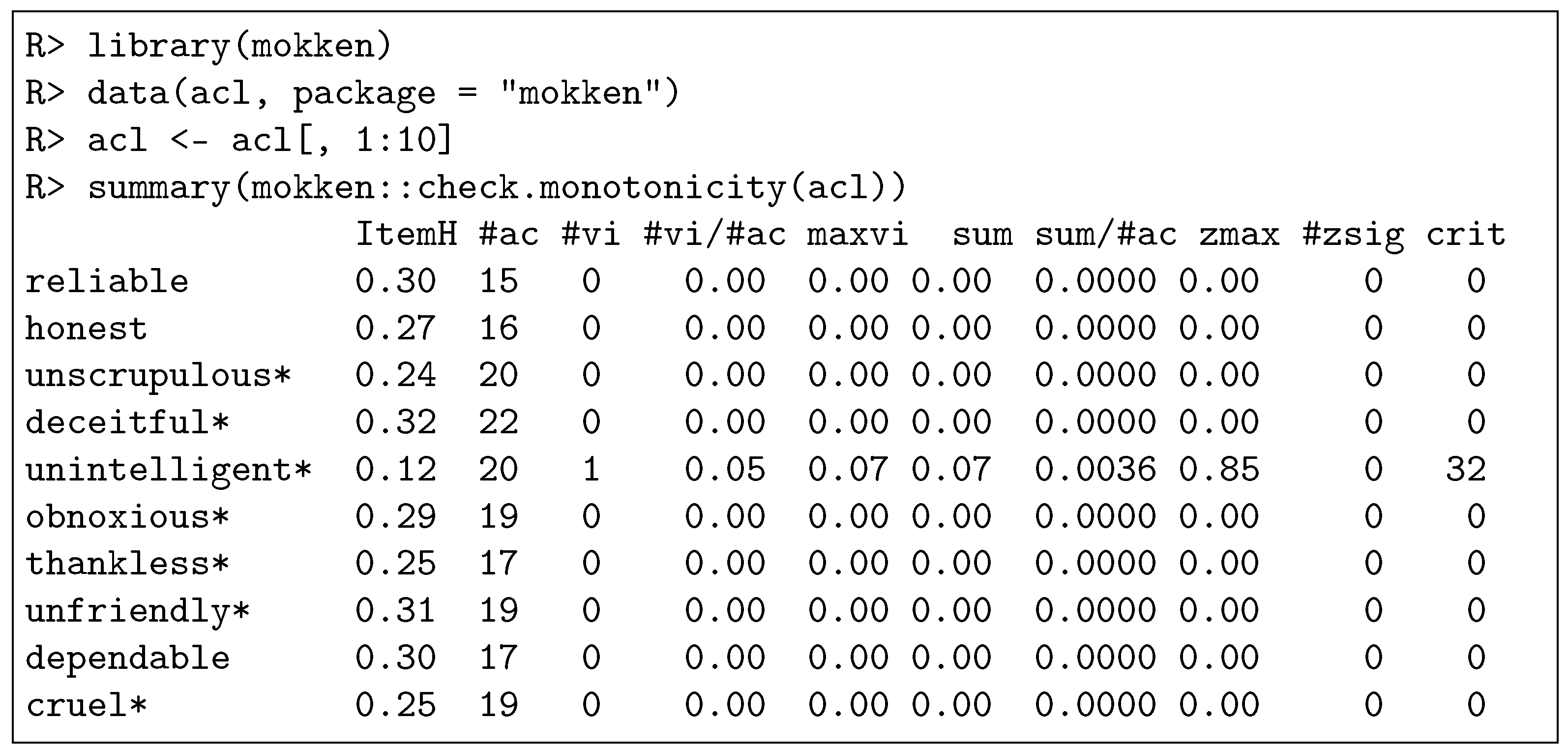
Figure 3.
Summary output of check.iio of the R package mokken for the first 10 items of the internal data set acl. The structure of the output is similar to the structure of the output of check.monotonicity (Figure 2). Note that 4 items belong to an item pair that shows a significant violation of manifest IIO (column #tsig). In addition, an asterisk indicates a negatively worded item, the software generates a list of items such that if they are removed, the resulting item set satisfies manifest IIO (not shown). ‘R>’ denotes the R prompt.
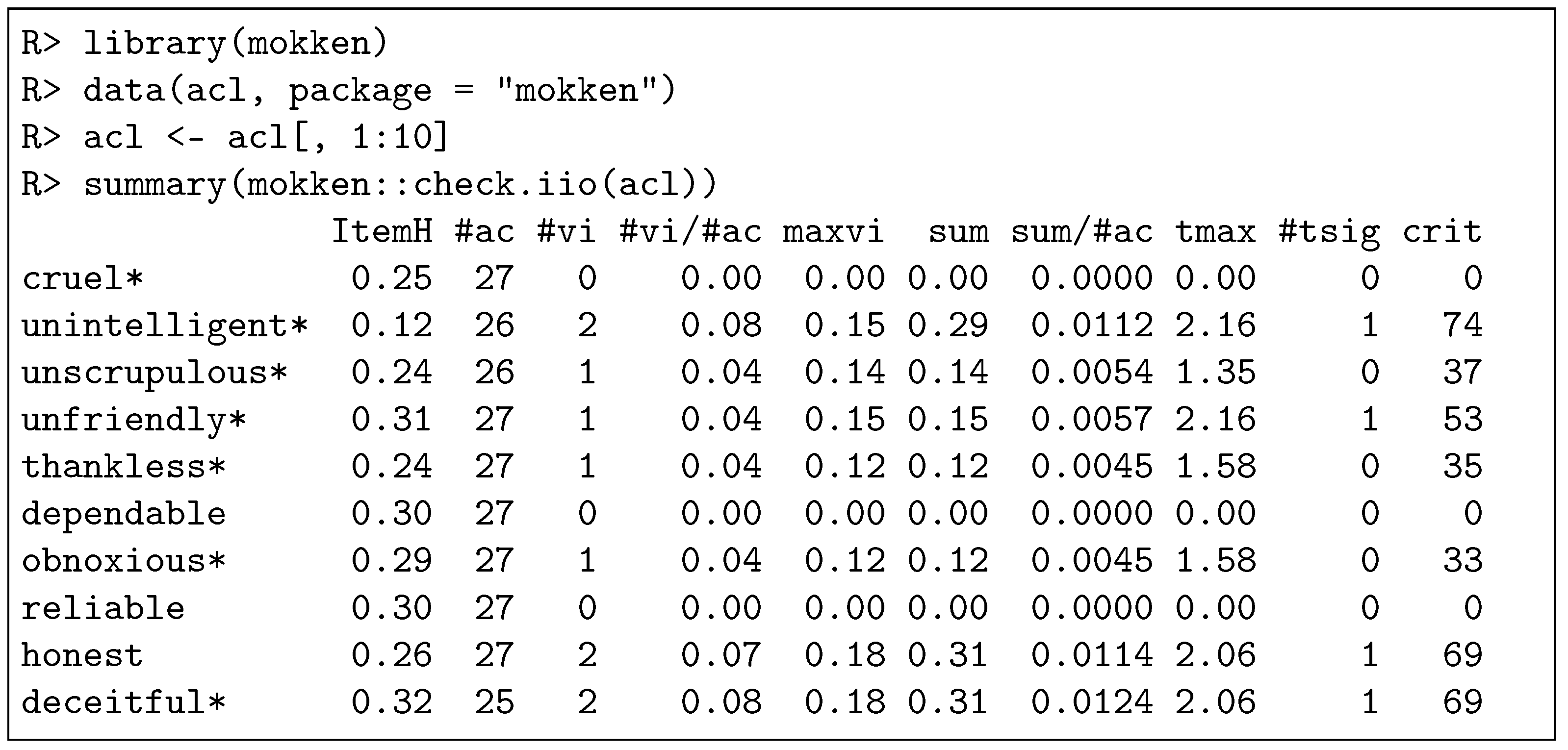
Figure 4.
MO = monotonicity. Level 1 item response functions (solid curves) and level 2 item response functions for (dashed curves), 0.5 (dash-dotted curves), 0.8 (dotted curves), for the small (left panel) and large (right panel) violation condition of monotonicity. The item response function of level 2 for is identical to the item response function of level 1.

Figure 5.
IIO = invariant item ordering. Level 1 item response functions (solid curves) and level 2 item response functions for values of 0.2 (dashed curves), 0.5 (dash-dotted curves), 0.8 (dotted curves), for the small (left panel) and large (right panel) violation conditions of IIO. The item response function of level 2 for is identical to the item response function of level 1.


Table 1.
False-positive counts for method manifest monotonicity.
| Indicator | Violation | S | Level 1 | Level 2 | |||
|---|---|---|---|---|---|---|---|
| #vi/#ac | None | 50 | 0.003 | 0.005 | 0.010 | 0.015 | 0.032 |
| 200 | 0.003 | 0.004 | 0.006 | 0.012 | 0.019 | ||
| #zsig | None | 50 | 0.001 | 0.000 | 0.000 | 0.000 | 0.000 |
| 200 | 0.001 | 0.000 | 0.000 | 0.000 | 0.000 | ||
Table 2.
Sensitivity counts for method manifest monotonicity.
| Indicator | Violation | S | Level 1 | Level 2 | |||
|---|---|---|---|---|---|---|---|
| #vi/#ac | Small | 50 | 0.334 | 0.511 | 0.443 | 0.297 | 0.246 |
| 200 | 0.325 | 0.477 | 0.398 | 0.285 | 0.241 | ||
| Large | 50 | 0.726 | 0.737 | 0.731 | 0.701 | 0.567 | |
| 200 | 0.731 | 0.751 | 0.752 | 0.729 | 0.625 | ||
| #zsig | Small | 50 | 1.466 | 0.000 | 0.000 | 0.000 | 0.000 |
| 200 | 1.354 | 0.255 | 0.017 | 0.000 | 0.001 | ||
| Large | 50 | 7.677 | 0.111 | 0.000 | 0.000 | 0.000 | |
| 200 | 7.803 | 4.847 | 2.491 | 0.335 | 0.021 | ||
Table 3.
False-positive counts for method manifest invariant item ordering.
| Indicator | Violation | S | Level 1 | Level 2 | |||
|---|---|---|---|---|---|---|---|
| #vi/#ac | None | 50 | 0.007 | 0.009 | 0.010 | 0.010 | 0.008 |
| 200 | 0.006 | 0.007 | 0.006 | 0.007 | 0.007 | ||
| #tsig | None | 50 | 0.000 | 0.001 | 0.003 | 0.002 | 0.004 |
| 200 | 0.000 | 0.001 | 0.003 | 0.000 | 0.001 | ||
Table 4.
Sensitivity counts for method manifest invariant item ordering.
| Indicator | Violation | S | Level 1 | Level 2 | |||
|---|---|---|---|---|---|---|---|
| #vi/#ac | Small | 50 | 0.322 | 0.376 | 0.344 | 0.309 | 0.251 |
| 200 | 0.325 | 0.377 | 0.342 | 0.305 | 0.257 | ||
| Large | 50 | 0.507 | 0.510 | 0.488 | 0.468 | 0.408 | |
| 200 | 0.520 | 0.524 | 0.521 | 0.496 | 0.449 | ||
| #tsig | Small | 50 | 0.380 | 0.671 | 0.556 | 0.379 | 0.189 |
| 200 | 0.384 | 0.668 | 0.534 | 0.350 | 0.221 | ||
| Large | 50 | 1.658 | 1.961 | 1.757 | 1.505 | 1.011 | |
| 200 | 1.694 | 1.901 | 1.786 | 1.526 | 1.202 | ||
Disclaimer/Publisher’s Note: The statements, opinions and data contained in all publications are solely those of the individual author(s) and contributor(s) and not of MDPI and/or the editor(s). MDPI and/or the editor(s) disclaim responsibility for any injury to people or property resulting from any ideas, methods, instructions or products referred to in the content. |
© 2023 by the authors. Licensee MDPI, Basel, Switzerland. This article is an open access article distributed under the terms and conditions of the Creative Commons Attribution (CC BY) license (https://creativecommons.org/licenses/by/4.0/).
Share and Cite
MDPI and ACS Style
Koopman, L.; Zijlstra, B.J.H.; Van der Ark, L.A. Evaluating Model Fit in Two-Level Mokken Scale Analysis. Psych 2023, 5, 847-865. https://doi.org/10.3390/psych5030056
AMA Style
Koopman L, Zijlstra BJH, Van der Ark LA. Evaluating Model Fit in Two-Level Mokken Scale Analysis. Psych. 2023; 5(3):847-865. https://doi.org/10.3390/psych5030056
Chicago/Turabian StyleKoopman, Letty, Bonne J. H. Zijlstra, and L. Andries Van der Ark. 2023. "Evaluating Model Fit in Two-Level Mokken Scale Analysis" Psych 5, no. 3: 847-865. https://doi.org/10.3390/psych5030056