Abstract
This paper presents a study of an automated system for identifying planktic foraminifera at the species level. The system uses a combination of deep learning methods, specifically convolutional neural networks (CNNs), to analyze digital images of foraminifera taken at different illumination angles. The dataset is composed of 1437 groups of sixteen grayscale images, one group for each foraminifera specimen, that are then converted to RGB images with various processing methods. These RGB images are fed into a set of CNNs, organized in an ensemble learning (EL) environment. The ensemble is built by training different networks using different approaches for creating the RGB images. The study finds that an ensemble of CNN models trained on different RGB images improves the system’s performance compared to other state-of-the-art approaches. The main focus of this paper is to introduce multiple colorization methods that differ from the current cutting-edge techniques; novel strategies like Gaussian or mean-based techniques are suggested. The proposed system was also found to outperform human experts in classification accuracy.
1. Introduction
Image classification is a very complex task that has witnessed massive improvement in the past decade, thanks to hardware advancements and the application of deep learning. Because this new technology is a repetitive and non-creative process, it is well-suited for automation. One of the best deep learners for images is a family of learners called convolutional neural networks (CNNs). CNNs have already proven their efficacy and efficiency at image classification in many studies [1]; however, the stochastic nature of neural networks (NNs) leads to results that are influenced by a fair share of randomness [2]. Ensemble learning (EL) is a widely used implementation that combines results from different heuristic algorithms to achieve better performance and higher consistency, reducing the individual random component of each algorithm.
This paper proposes a practical application of EL to the classification problem presented in [3], which was to train a CNN for foraminifera classification, a task of high interest for industrial and research purposes [4]. Species of planktic foraminifera are paleo-environmental bioindicators, whose radiocarbon measurements are used to infer parameters like global ice volume, temperature, salinity, PH, and nutrient content of ancient marine environments. Foraminifera classification is usually performed by groups of humans, ranging in size from 500 to 1000 individuals. As a result, foraminifera classification is a very repetitive, resource-intensive, and time-consuming process. Since the early 1990s, there have been several attempts to automate this task [5]. Although strides were made in this direction, most methods still required strong human supervision. In 2004, however, the neural network SYRACO2 was developed to identify single-celled organisms automatically, and was shown to perform reliably [6]. In 2017 CNNs were applied to diatom identification with great success [7]. With further development, CNNs should be able to take over the arduous process of foraminifera classification.
Transfer learning, which takes a pre-trained CNN as the baseline for training on another dataset of images, typically a smaller one, is yet another technique that can be employed to improve classification accuracy at the end of the training process [8].
Our goal is to use these techniques to improve the classification accuracy on the same dataset presented in [3]. This dataset is composed of 1437 groups of sixteen grayscale images of foraminifera taken at different lighting angles and separated into seven classes, six labeled, shown in Figure 1, and one “other”. Several RGB colorization approaches were used to generate different sets of colored images that became the inputs for a set of CNN architectures that formed the EL environment. The authors of [3] employed a fusion of ResNet50 and Vgg16, using colorization methods based on intensity percentiles in the sixteen grayscale channels.
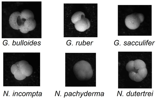
Figure 1.
Visual comparison of the six labelled species of foraminifera in the dataset.
This paper proposes several alternative colorization methods that deviate from the state of the art [9] but still achieve remarkable ensemble results. New approaches such as Luma scaling, HSV color space mapping, and Gaussian or mean-based techniques are applied to CNN architectures to extend the study presented in [3]. The results of this study show that a diverse set of CNN models trained on different colorized images improves the system’s performance compared to other state-of-the-art approaches. The proposed system is also shown to outperform human experts in classification accuracy.
Related Work
Mitra et al. [3] first proposed this deep-learning-based (DL) framework in 2019, achieving discrete success, but averaging just below the performance of human experts. Their approach did not put much focus on the pre-processing colorization part, missing a potential avenue for improving performance even further.
It is important to note that the application of multi-grayscale channels to RGB colorization is not limited to the field of foraminifera classification, but can be applied in other domains as well. Some example applications include remote sensing [10,11], where multispectral images are often represented in grayscale, and medical imaging, where grayscale images are commonly used in CT scans and MRI images [12], which can then be applied to a wide range of classification problems, like clinical diagnosis and image-guided interventions and procedures [13].
It has been found that appropriate image fusion and colorization of multi-band representations can lead to improved information quantity carried per image [14], meaning that, with opportune pre-processing methods, a DL approach could achieve better performance, as shown in studies like [15].
The use of RGB colorization in these domains has already been shown to improve the performance of classification tasks and enhance the interpretability of the results. For example, in medical imaging, converting grayscale images to RGB can highlight certain features in the images that were not as noticeable in grayscale, potentially leading to improved diagnosis accuracy [16]. Similarly, in remote sensing, RGB colorization can help highlight different features in the image, such as vegetation or water bodies, or gesture recognition [17], improving CNNs’ results. Thus, the methods proposed here should also increase classification accuracy in other domains that use grayscale images. Furthermore, our methods should work well for the image fusion of different grayscale pictures obtained from multispectral analysis [10,11], or from polarized/filtered light sources on objects that may be difficult to capture in the typical visible spectrum.
Using ensemble learning to build different neural networks based on different image fusion techniques has also been shown to increase performance across the board, reaching far better results than individual approaches [18,19]. This suggests that combining different colorization techniques in ensembles should also help increase key performance indicators for the classification problem at hand.
The source code for the system, written in MATLAB, is available at a provided GitHub repository: https://github.com/LorisNanni accessed on 12 July 2023.
2. Materials and Methods
The dataset used can be found at https://doi.pangaea.de/10.1594/PANGAEA.897873 accessed on 12 July 2023.
It is composed of a total of 1437 samples, divided into the following classes:
- 178 images are G. bulloides;
- 182 images are G. ruber;
- 150 images are G. sacculifer;
- 174 images are N. incompta;
- 152 images are N. pachyderma;
- 151 images are N. dutertrei;
- 450 images are “rest of the world”, i.e., they belong to other species of planktic foraminifera.
The initial images were obtained using a reflected light binocular microscope, each taken with a light shining from the side at 22.5° intervals, using an AmScope SE305R-PZ binocular microscope at 30× magnification [3]. For every sample of foraminifera, sixteen grayscale pictures were taken at different illumination angles. The resolution of the images can vary per sample, but most are around 450 × 450 pixels. Upon manual inspection, the starting illumination angle for the sixteen images seems to change partially for different classes of foraminifera in the naming scheme used to sort the pictures. We believed the start angle could lead to biased results in classification if a specific class always had the same starting angle compared to the others. This problem was addressed, when pre-processing the images, by randomly sorting them while keeping the relative illumination angles ordered, to avoid the insertion of bias within methods that leverage the light positional information.
2.1. CNN Ensemble Learning
The theory behind ensemble learning is based on a simple idea: by combining different models, it should be possible to produce better and more reliable results. Ensembles can be constructed on four different levels:
- Data level: by splitting the dataset into different subsets;
- Feature level: by pre-processing the dataset with different methods;
- Classifier level: by training different classifiers on the same dataset;
- Decision level: by combining the decisions of multiple models.
Ensembles work best when applied to significantly diverse models [20]. In this work, we construct ensembles by applying different pre-processing approaches, detailed in Section 3, for representing the input images as RGB images. The images generated by these approaches are used to train multiple networks whose decisions are finally combined using the sum rule.
CNNs were first introduced in the 1980s by the French researcher Yann LeCun [21], and were shown to perform well throughout the 1990s [22,23]. In the last decade, however, due to the advent of big data and GPU computing, the performance of CNNs has increased to the point that, in computer vision and image recognition, CNNs are now considered state-of-the-art.
As with every other type of neural network, the structure of a CNN is divided into three components: an input layer, which, in a CNN architecture, is usually a volume of n × n × 3 neurons directly connected to the input of an image’s pixels, hidden layers that utilize shared weights and local connections, and a fully connected output layer.
CNNs take as input three dimensional tensors, most often used to represent images of size W × H × C, with the terms being, respectively, the width and height of the image, and the number of channels associated with each pixel, which can hold information such as RGB color values, alpha channel transparency, depth, and more.
The output of a CNN is given by the final fully connected layer, and it returns a probability or confidence score for each of the possible labels of the classification problem. The label with the highest probability is chosen as the network’s final prediction.
In this work, we use the ResNet50/ResNet18/GoogleNet/MobileNetV2 topologies pretrained using ImageNet, which is fine-tuned further for 20 epochs with a learning rate of 0.001 and a batch size of 30.
The Vgg16 architecture was also considered for this study, but the lack of residual connections and the large number of hidden layers made the training very slow when compared to ResNet-based architectures, so we decided to omit it from this ensemble.
This is because the residual connections, shown in Figure 2, allow information from previous layers to carry over to deeper layers, which enables the network to express a much larger function class with less layers when compared to standard deep CNNs [24].
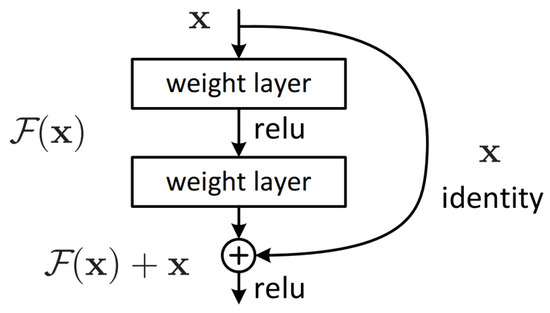
Figure 2.
Residual block from ResNet [24].
2.2. Image Pre-Processing
Each image in the dataset, presented in [3] and described in more detail in Section 2, comes in the form of sixteen grayscale pictures of the same foraminifera subject. The dataset, size 1437 samples, is divided into seven classes: one for each of the six species of foraminifera that are the subject of this study, plus one “other” class. Each class has approximately 150 entries, except for “other”, which has 450.
Since we use pre-trained networks, and their inputs are expected to be RGB images, the first step in our pipeline will be to generate CNN-compatible inputs starting from the dataset.
Multiple ways for completing this task were tested; in the end, we settled on a combination of five:
- The “percentile” method presented in [3], here called “baseline”, see Figure 3;
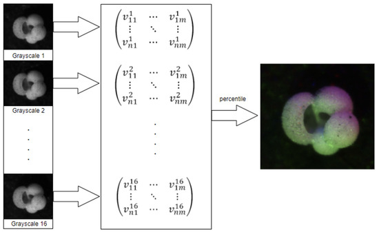 Figure 3. Percentile pre-processing pipeline, sourced from [25].
 - A “Gaussian” image processing method that encodes each color channel based on the normal distribution of the grayscale intensities of the sixteen images;
- Two “mean-based” methods focused on utilizing an average or mean of the sixteen images to reconstruct the R, G, and B values;
- The “HSVPP” method, that utilizes a different color space composed of hue, saturation, and value of brightness information, see Figure 4;
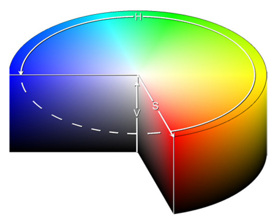 Figure 4. HSV color space representation as found on [26].
 - The “GraySet” method, which takes each of the 16 grayscale images for every pattern, and creates 16 RGB images by copying grayscale values in every color channel.
An illustration of the resulting images can be found in Figure 5. A discussion of the five methods is provided below.
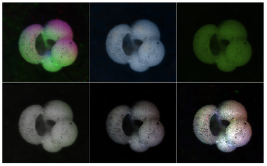
Figure 5.
Examples of the six colorization methods. In the top row from left to right: percentile, Gaussian, and luma scaling images; In the bottom row from left to right: means reconstruction, HSV, and HSVPP images.
2.2.1. Percentile
Percentile is the most straightforward method for generating an RGB image. As presented in [3], the sixteen individual grayscale values for each pixel are used to calculate the 10th percentile, median, and 90th percentile. These three values are then mapped to the RGB channels to generate a single color composite.
To speed up the process, we use the nearest rank method: the list of sixteen grayscale values is sorted in ascending order, after which the P-th percentile element is selected by extracting the value of cell n, where
Since our input vectors are always the same size, the sixteen values are sorted, and the three values of n selected here are 2, 8, and 15.
The percentile pre-processing pipeline, see Figure 3, works as follows:
- Read the sixteen images;
- Populate a matrix with the grayscale values;
- For each pixel, extract its sixteen grayscale values into a list;
- Sort the list;
- Use elements 2, 8, and 15 as RGB values for the new image.
A few variations of this method were also tested (the 20th/80th/median, for example), but they were discarded due to their performance being slightly worse than the original, losing out on 1–2% of accuracy per single-run training cycle on average.
2.2.2. Gaussian
The Gaussian method for image processing tries to find the optimal way to fit the sixteen grayscale image values at position x, represented as the vector , in a normal distribution, using the fitdist method in MATLAB.
The fitting of sixteen values into a normal distribution is independent of their ordering, thereby ensuring that no bias from the order of lighting angles is encoded into the colorized images.
Once the distribution is computed, the R, G, and B values of the colorized image are assigned as follows:
Given the Gaussian random variable fit from ,
If any assigned value is negative or exceeds 255, it is thresholded to the nearest valid color intensity value 0 or 255.
2.2.3. Mean-Based
With mean-based methods, the main idea is to address the lack of ordering in the lighting angle of the various samples by combining the sixteen pictures of each sample into a single image that approximates the information contained in the grayscale images. The mean is then used to determine each of the RGB color values. The advantage of approaches like these is that they can be computed relatively quickly compared to more involved image colorization techniques. The techniques used to determine the RGB color values are detailed in the following sub-sections. Given a set of values , the following means were calculated:
2.2.4. Luma Scaling
Considering that a mean grayscale image can be viewed as containing only luminosity information, it follows that a possible way to assign RGB values and colorize the picture would be to try to compute a color value according to its perceived luminosity. With images close to the resolution of standard definition (SD) television, which is 704 × 480 pixels, the luma scaling approach attempts to encode luma information in the component video following values used by the BT.601 standard. The formula for recovering luma information is:
This formula weighs the primary colors based on their brightness, with green the brightest component and blue the dimmest. The luma scaling images are obtained from these weights, which are multiplied by the mean image to obtain the intensity value for each color channel; the result is a basic recoloring obtained by computing the following:
Given the pixel at position x, let be the array of sixteen values of the grayscale intensity of the sixteen images in that position; the colored reconstruction is obtained as follows:
- ;
- ;
- .
2.2.5. Means Reconstruction
This approach utilizes an important relationship between the three different means. Knowing that the order of luminosity between the three primary colors is , and given an array of real numbers S, the following relationship holds true:
Given the vector of sixteen grayscale images of each sample at a given pixel position x, the means reconstruction approach maps every mean to a color channel according to the established order as follows:
- ;
- ;
- .
2.2.6. HSVPP: Hue, Saturation, Value of Brightness + Post-Processing
This method utilizes an alternative representation of RGB information. Instead of encoding each RGB color channel separately, each pixel is encoded with three different values that represent coordinates in the HSV color space, as illustrated in Figure 4.
The three values are computed for all sixteen grayscale images in the following manner:
- H is assigned based on the index of the image, giving each a different color hue;
- S is set to 1 by default, for maximizing diversity between colors;
- V is set to the grayscale image’s original intensity, i.e., its brightness.
Since the ordering of the lighting angles differs across the classes, the sixteen images are shuffled randomly to prevent bias before computing H. Shuffling ensures that the network does not discriminate classes based on the order of lightning angles in the post-processed images.
After obtaining sixteen images of different colors, they are fused into a single RGB image by converting the HSV representation to RGB, then by summing the squared intensity of each channel together into a single colorized image.
Finally, it is possible to enhance the resulting images with some post-processing, mainly by increasing the brightness of the darker colors and reducing haze for a sharper image. Once this post-processing is complete, the HSVPP dataset is ready to be fed to the network.
2.2.7. GraySet
The GraySet method consists of taking each one of the 16 grayscale images of a pattern, and creating 16 RGB images (for each training and test patterns) by copying the grayscale values into each of the three color channels.
In more detail, each one of the sixteen grayscale images for a given pattern, which we will call through , is encoded into an RGB image following the simple rule:
- for the first RGB image;
- for the second one;
- And so on, up to for the last image in the pattern.
As described earlier, this procedure is applied to both training and test patterns. For each test pattern, we have sixteen images, then sixteen scores for each trained CNN; these sixteen scores are combined by the average rule.
2.3. Training
Once the augmented dataset is built, networks are trained using a pre-trained ResNet50, which, as the name suggests, is a 50-layer CNN. The input layer is a 224 × 224 × 3 zero-pad layer. There are 48 hidden layers, two of which are a max and an average pool, respectively. Networks of the ResNet family utilize residual blocks to maximize depth while diminishing the number of parameters [8]. We also used ResNet18, which works much the same but with 18 layers, GoogLeNet [27], which is 22 layers deep, and MobileNetv2 [28], which is composed of 20 layers. All networks used take 224 × 224 × 3 images as input, so the inputs are resized as such using Matlab’s standard interpolation. This almost always changes the pictures’ original resolution, making them smaller, so we can reasonably assume that some detail is lost in the process. Adapting the networks to take variable input resolution might be a possible future development for this approach.
All networks were pre-trained with the open-source image dataset ImageNet, which contains millions of labelled images. Hyperparameters for all networks were set as follows:
- Mini Batch Size: 30;
- Max Epochs: 20;
- Learning Rate: 10−3.
The main benefit of a pre-trained network is transfer learning. A modern neural network can carry over some of the knowledge gained in previous training cycles on a particular dataset when retraining it on a different dataset [8]. This carry-over of information is especially pronounced in deep learning models, because they operate on a wide array of weights and features. Transfer learning significantly reduces the time and number of images needed to train the networks, an advantage when working with relatively small datasets. All layers are tuned, none frozen.
The output layer of the pretrained networks has to be adapted to accommodate the task of foraminifera classification. Thus, all the output layers were replaced with fully connected SoftMax layers of seven neurons, one for each class of foraminifera available in the dataset. Images of the dataset were also resized to match the dimensions of the input layers.
By replacing the last layer with a seven-neuron SoftMax layer, the outputs form a vector , whose values (scores) are:
By diversifying the models, the information processed by each is different. Score fusion is a method that combines the confidence values of each model to build a more robust prediction. The fusion technique used here is the sum rule [19], defined as:
where is the number of models and the size of each confidence vector . The sum rule is one of the best fusion methods because it does not suffer from potentially destructive operations like multiplication by zero.
3. Results
The testing protocol for the dataset is the 4-fold cross-validation, and the performance metric is the F-score (), defined as:
where , , are, respectively, the total number of True positives and the False positive/negative predictions made by the model.
In Table 1, we compare our ensemble, coupled with different network topologies, with that proposed in [3]. With X(y), we report the performance of y CNNs trained with the X RGB approach for colorizing the images.

Table 1.
F1 scores across the specified training cycles.
In the column ResNet50_DA we couple the ResNet50 with a data augmentation approach. The tested data augmentation takes a given image, and randomly reflects it top–bottom and left–right for two new images. The third transform linearly scales the original image along both axes with two factors randomly extracted from the uniform distribution [1,2].
The conclusions that can be obtained from the results reported in Table 2 are the following:
Table 2.
Precision, recall, accuracy and F1 score comparison between [3] and the best ensemble presented in the paper.
- The best-performing ensemble produces results that significantly improve those obtained by the method presented in [3] (percentile), whose F1 score was reported as 85%;
- Among stand-alone approaches the best performance is obtained by GraySet;
- It appears that, in general, increasing the diversity of the ensemble yields better results. The approaches combining multiple pre-processed images sets consistently rank higher in F1 scores than any individual method, iterated ten times. Combining fewer iterations of all the approaches yielded the best results overall. Similar conclusions are obtained with the different topologies;
- The ensemble based on ResNet50_DA obtains performance similar to the one based on ResNet50, but clearly data augmentation improves the stand-alone approaches.
The breakdown of the 4-fold classification on the full dataset is presented in Figure 6 as a confusion chart, where we can see the number of true positives, false positives, and false negatives. The N. Incompta species was classified correctly the least which, alongside the high number of false positives predicted, is consistent with the classification rate in [3], although it found the false negatives to be the larger issue.
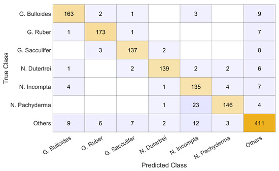
Figure 6.
Confusion chart of the 4-fold cross validation results obtained by our ensemble.
4. Discussion
Comparing the final results of the ensemble with the study reported in [3], the precision averaged across the six labelled classes achieved by six human experts ranged from 59% to 83%, with a mean of 74%. In contrast, five human novices ranged from 49% to 65%, with 56% on average. The ensemble approach proposed in [3] was found to achieve an average precision of 80%, which is comparable to that of the experts. The best ensemble presented in Table 1, which is percentile(1) + Gaussian(1) + luma scaling(1) + means reconstruction(1) + HSVPP(1) + GraySet(5), was found to achieve an average precision of 91%, a much better average than that of the experts and higher than any of them individually.
Similar results have been obtained for recall and the F1 score, which was always averaged across the six labelled classes. The six experts achieved recall between 32% and 83% (mean 60%), while the novices scored 47–64% (mean 53%). The ensemble proposed in [3] (ResNet50 + Vgg16) reported an average recall of 82%, while our ensemble reached 90%. The F1 score of the six experts ranged from 39% to 83% (mean 63%), the five novices obtained F1 scores between 47% and 63% (mean 53%), and the [3] reported an average of 85%. The ensemble presented in this paper scored 90.6%. These results are illustrated in Table 2.
On a finer level, we have also charted the precision, recall and F1 scores across all the different classes in our study, as seen in Table 3.
Table 3.
Precision, recall and F1 score of the best ensemble across all classes of the dataset.
In both precision and F1 score, N. incompta comes out the lowest by a significant margin, achieving 0.77 in precision, while the other six classes average 0.94; the F1 score for N. incompta is 0.83, while the other six classes average 0.92. N. pachyderma has the poorest recall, achieving 0.84, while the other six classes average 0.92. In contrast, the highest recall and F1 score were achieved on the G. ruber class, alongside the third-highest precision, which may indicate it has features that are easier to distinguish than all the others.
Out of the false positives for G. ruber, three were G. sacculifer, two were G. bulloides, and six were Others, while the false negatives were only misclassified as G. sacculifer or as Other. The differences and similarities between the false positives and real data are illustrated in Figure 7.
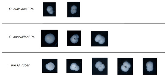
Figure 7.
Visual comparison of false positives (FPs) in the classification of G. ruber with hand-picked true samples.
The highest precision was instead achieved on the N. dutertrei class, along with the second-highest F1 score and third-highest recall. Only six patterns were misclassified as false positives, of which two were G. sacculifer, one was N. incompta, and one N. pachyderma, as well as two Others, shown in Figure 8.
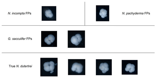
Figure 8.
Visual comparison of false positives (FPs) in the classification of N. dutertrei with hand-picked true samples.
It is important note that all the performance indicators for our method achieved scores higher than 77%, while in [3] some classes like N. dutertrei had precision less than 70%.
The main disadvantage of the proposed ensemble is the increase in computational time; the preprocessing approaches are not computationally expensive, the main computational requirement is the inference with the set of CNNs. In any case, with a Titan RTX 24 GB, we can classify a batch of one thousand images in 1.945 s.
Using the Q-statistic [20], we demonstrate that the errors made by the individual classifiers employed in our ensemble exhibit (partial) independence. The Q-statistic ranges between −1 and 1 for two classifiers. A value of Q = 0 indicates statistical independence between the classifiers. When classifiers tend to correctly identify the same patterns, Q > 0, whereas classifiers that make errors on distinct patterns have Q < 0. The average Q-statistic among the classifiers that belong to “percentile(1) + Gaussian(1) + luma scaling(1) + means reconstruction(1) + HSVPP(1) + GraySet(5)” is 0.8369, instead the average Q-statistic among the classifiers that belong to GraySet(10) is 0.9776; it is clear that varying the preprocessing approach allows for lowering the value of the Q-statistic, creating a more performing ensemble.
5. Conclusions
Although the sample size of the experiment is small, the impact of ensemble learning on the problem is definitely noticeable. There are, however, a few points of concern. The dataset only contained ~1500 images divided into seven classes of foraminifera, a problem we addressed with transfer learning. Nonetheless, the scope of the experience was limited to a very small portion of the real-world problem of foraminifera classification. We can, however, safely assume that with more samples per class, performance could be enhanced even further. What we are uncertain about, without experimental data, is how the model would respond to a larger set of classes. Image preprocessing and classification on multiple CNNs are very time-consuming tasks. Because our models were run on sub-optimal machines, our focus was directed toward maximizing accuracy while neglecting the time it took for training.
The strength of the presented approach obviously lies in the improved accuracy of the predictions, achieving an 8% improvement in F1 score over human experts, while relying on no additional data. Achieving such performance makes this model a valuable tool for this task.
However, the required pre-processing of the images is much more demanding, both in terms of inference time and computation required, but remains within feasible terms.
Such a huge increase in key performance indicators is still well worth the computational complexity tradeoff, demonstrating the effectiveness of a robust ensemble over a single neural network for image classification problems.
A possible future development of the project is the application of the technique used to generate an approximate normal map of an object from grayscale images with lights coming from the four cardinal directions. Since normal maps are used in 3D computer graphics to fake details such as bumps, dents, and lighting, without the need for added geometry, these results could also be used to generate entirely new images with new lighting conditions, colors, and viewpoints without the need of the human labor usually needed to increase the size of the dataset.
As also discussed in Section 2.3, other future developments might include further adaptations of the input layers of the pre-trained networks, like allowing for variable resolution images, or modifying the input layer so that the network becomes capable of taking 16-channel inputs, which would necessitate training some layers from scratch to utilize the pre-trained backbone.
Author Contributions
Conceptualization, L.N. and G.F.; methodology, L.N.; software, R.B., E.F., L.N. and G.F.; investigation, L.N., S.B., R.B., E.F. and G.F.; writing—original draft preparation, R.B., E.F., S.B., G.F. and L.N.; writing—review and editing, S.B., G.F. and L.N. All authors have read and agreed to the published version of the manuscript.
Funding
This research received no external funding.
Data Availability Statement
Publicly available datasets were analyzed in this study. This data can be found here: https://doi.pangaea.de/10.1594/PANGAEA.897873 accessed on 12 July 2023.
Acknowledgments
Through their GPU Grant Program, NVIDIA donated the TitanX GPU used to train the CNNs presented in this work.
Conflicts of Interest
The authors declare no conflict of interest.
References
- Li, Z.; Liu, F.; Yang, W.; Peng, S.; Zhou, J. A Survey of Convolutional Neural Networks: Analysis, Applications, and Prospects. IEEE Trans. Neural Netw. Learn. Syst. 2022, 33, 6999–7019. [Google Scholar] [CrossRef]
- Menart, C. Evaluating the variance in convolutional neural network behavior stemming from randomness. Proc. SPIE 11394 Autom. Target Recognit. XXX 2020, 11394, 1139410. [Google Scholar] [CrossRef]
- Mitra, R.; Marchitto, T.M.; Ge, Q.; Zhong, B.; Kanakiya, B.; Cook, M.S.; Fehrenbacher, J.D.; Ortiz, J.D.; Tripati, A.; Lobaton, E. Automated species-level identification of planktic foraminifera using convolutional neural networks, with comparison to human performance. Mar. Micropaleontol. 2019, 147, 16–24. [Google Scholar] [CrossRef]
- Edwards, R.; Wright, A. Foraminifera. In Handbook of Sea-Level Research; Shennan, I., Long, A.J., Horton, B.P., Eds.; Wiley: Hoboken, NJ, USA, 2015. [Google Scholar] [CrossRef]
- Liu, S.; Thonnat, M.; Berthod, M. Automatic classification of planktonic foraminifera by a knowledge-based system. In Proceedings of the Tenth Conference on Artificial Intelligence for Applications, San Antonio, TX, USA, 1–4 March 1994; pp. 358–364. [Google Scholar] [CrossRef]
- Beaufort, L.; Dollfus, D. Automatic recognition of coccoliths by dynamical neural networks. Mar. Micropaleontol. 2004, 51, 57–73. [Google Scholar] [CrossRef]
- Pedraza, L.F.; Hernández, C.A.; López, D.A. A Model to Determine the Propagation Losses Based on the Integration of Hata-Okumura and Wavelet Neural Models. Int. J. Antennas Propag. 2017, 2017, 1034673. [Google Scholar] [CrossRef]
- Zhuang, F.; Qi, Z.; Duan, K.; Xi, D.; Zhu, Y.; Zhu, H.; Xiong, H.; He, Q. A Comprehensive Survey on Transfer Learning. Proc. IEEE 2021, 109, 43–76. [Google Scholar] [CrossRef]
- Huang, B.; Yang, F.; Yin, M.; Mo, X.; Zhong, C. A Review of Multimodal Medical Image Fusion Techniques. Comput. Math. Methods Med. 2020, 2020, 8279342. [Google Scholar] [CrossRef] [PubMed]
- Sellami, A.; Abbes, A.B.; Barra, V.; Farah, I.R. Fused 3-D spectral-spatial deep neural networks and spectral clustering for hyperspectral image classification. Pattern Recognit. Lett. 2020, 138, 594–600. [Google Scholar] [CrossRef]
- Zhang, X.; Ye, P.; Xiao, G. VIFB: A Visible and Infrared Image Fusion Benchmark. In Proceedings of the IEEE/CVF Conference on Computer Vision and Pattern Recognition (CVPR) Workshops, Seattle, WA, USA, 14–19 June 2020; pp. 104–105. [Google Scholar]
- James, A.P.; Dasarathy, B.V. Medical image fusion: A survey of the state of the art. Inf. Fusion 2014, 19, 4–19. [Google Scholar] [CrossRef]
- Hermessi, H.; Mourali, O.; Zagrouba, E. Multimodal medical image fusion review: Theoretical background and recent advances. Signal Process. 2021, 183, 108036. [Google Scholar] [CrossRef]
- Li, X.; Jing, D.; Li, Y.; Guo, L.; Han, L.; Xu, Q.; Xing, M.; Hu, Y. Multi-Band and Polarization SAR Images Colorization Fusion. Remote Sens. 2022, 14, 4022. [Google Scholar] [CrossRef]
- Moon, W.K.; Lee, Y.W.; Ke, H.H.; Lee, S.H.; Huang, C.S.; Chang, R.F. Computer-aided diagnosis of breast ultrasound images using ensemble learning from convolutional neural networks. Comput. Methods Programs Biomed. 2020, 190, 105361. [Google Scholar] [CrossRef] [PubMed]
- Maqsood, S.; Javed, U. Multi-modal Medical Image Fusion based on Two-scale Image Decomposition and Sparse Representation. Biomed. Signal Process. Control 2020, 57, 101810. [Google Scholar] [CrossRef]
- Ding, I.J.; Zheng, N.W. CNN Deep Learning with Wavelet Image Fusion of CCD RGB-IR and Depth-Grayscale Sensor Data for Hand Gesture Intention Recognition. Sensors 2022, 22, 803. [Google Scholar] [CrossRef] [PubMed]
- Tasci, E.; Uluturk, C.; Ugur, A. A voting-based ensemble deep learning method focusing on image augmentation and preprocessing variations for tuberculosis detection. Neural Comput. Appl. 2021, 33, 15541–15555. [Google Scholar] [CrossRef] [PubMed]
- Mishra, P.; Biancolillo, A.; Roger, J.M.; Marini, F.; Rutledge, D.N. New data preprocessing trends based on ensemble of multiple preprocessing techniques. TrAC Trends Anal. Chem. 2020, 132, 116045. [Google Scholar] [CrossRef]
- Kuncheva, L.I. Combining Pattern Classifiers. Methods and Algorithms, 2nd ed.; Wiley: Hoboken, NJ, USA, 2014. [Google Scholar]
- LeCun, Y.; Boser, B.; Denker, J.S.; Henderson, D.; Howard, R.E.; Hubbard, W.; Jackel, L.D. Backpropagation Applied to Handwritten Zip Code Recognition. Neural Comput. 1989, 1, 541–551. [Google Scholar] [CrossRef]
- Bengio, Y.; LeCun, Y. Convolutional Networks for Images, Speech, and Time-Series. In The Handbook of Brain Theory and Neural Networks; MIT Press: Cambridge, MA, USA, 1998; pp. 255–258. [Google Scholar]
- LeCun, Y.; Bottou, L.; Bengio, Y.; Haffner, P. Gradient-based learning applied to document recognition. Proc. IEEE 1998, 86, 2278–2324. [Google Scholar] [CrossRef]
- He, K.; Zhang, X.; Ren, S.; Sun, J. Deep residual learning for image recognition. In Proceedings of the IEEE Conference on Computer Vision and Pattern Recognition, Las Vegas, NV, USA, 27–30 June 2016; pp. 770–778. [Google Scholar] [CrossRef]
- Vallazza, M.; Nanni, L. Convolutional Neural Network Ensemble for Foraminifera Classification. Bachelor’s Thesis, University of Padua, Padua, Italy, 2022. Available online: https://hdl.handle.net/20.500.12608/29285 (accessed on 13 May 2023).
- Hue Saturation Brightness, Wikipedia, Wikimedia Foundation. Available online: https://it.wikipedia.org/wiki/Hue_Saturation_Brightness (accessed on 13 May 2023).
- Szegedy, C.; Liu, W.; Jia, Y.; Sermanet, P.; Reed, S.; Anguelov, D.; Erhan, D.; Vanhoucke, V.; Rabinovich, A. Going deeper with convolutions. In Proceedings of the IEEE Conference on Computer Vision and Pattern Recognition (CVPR), Boston, MA, USA, 7–12 June 2015; pp. 1–9. [Google Scholar] [CrossRef]
- Sandler, M.; Howard, A.; Zhu, M.; Zhmoginov, A.; Chen, L.C. MobileNetV2: Inverted Residuals and Linear Bottlenecks. arXiv 2019, arXiv:1801.04381. [Google Scholar] [CrossRef]
Disclaimer/Publisher’s Note: The statements, opinions and data contained in all publications are solely those of the individual author(s) and contributor(s) and not of MDPI and/or the editor(s). MDPI and/or the editor(s) disclaim responsibility for any injury to people or property resulting from any ideas, methods, instructions or products referred to in the content. |
© 2023 by the authors. Licensee MDPI, Basel, Switzerland. This article is an open access article distributed under the terms and conditions of the Creative Commons Attribution (CC BY) license (https://creativecommons.org/licenses/by/4.0/).