
Spatial Coherence Comparisons between the Acoustic Field and Its Frequency-Difference and Frequency-Sum Autoproducts in the Ocean


Abstract
:1. Introduction
2. Materials and Methods
2.1. Coherence and Coherence Length
2.2. Autoproducts
2.3. Matched-Field Processing
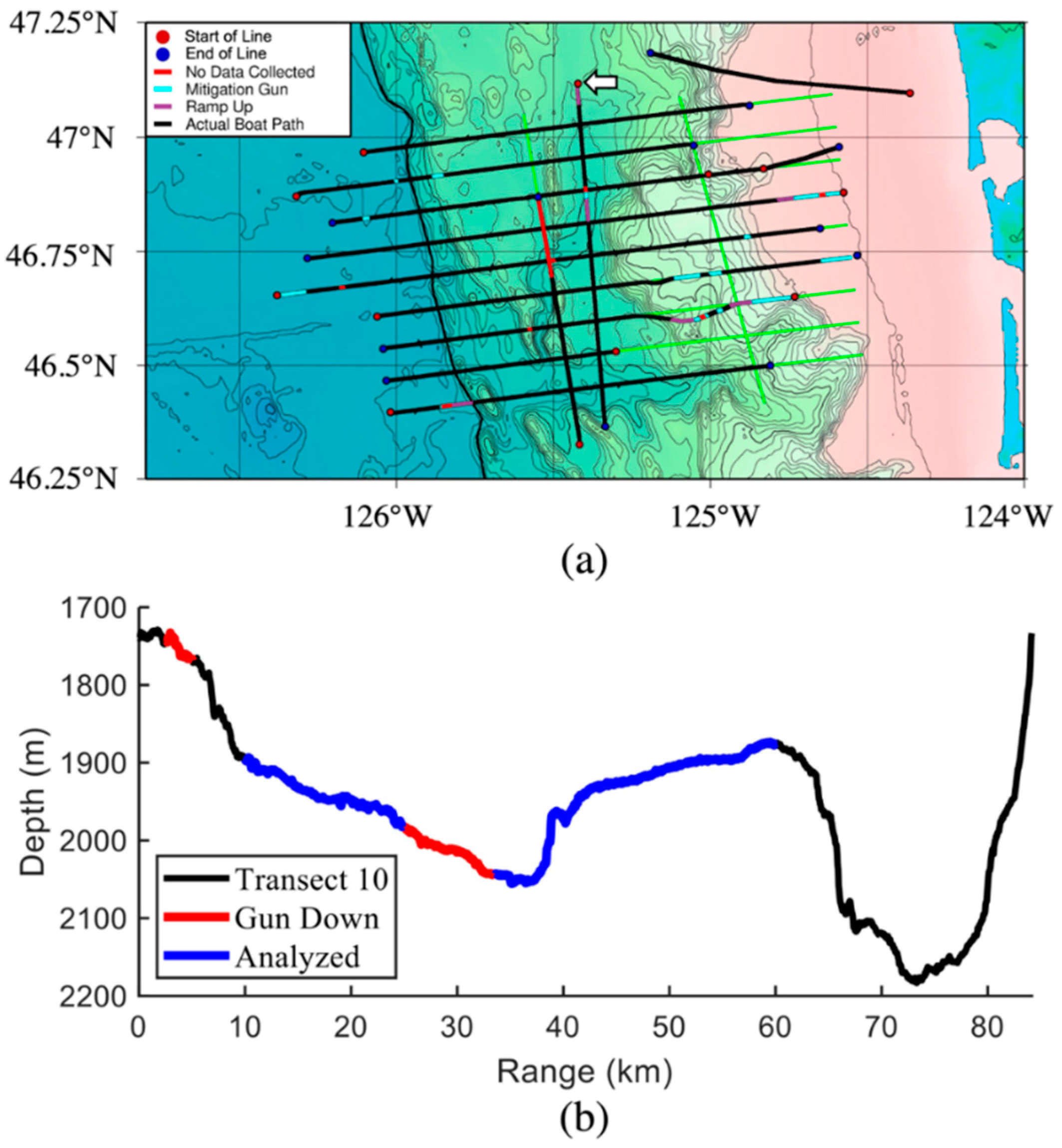
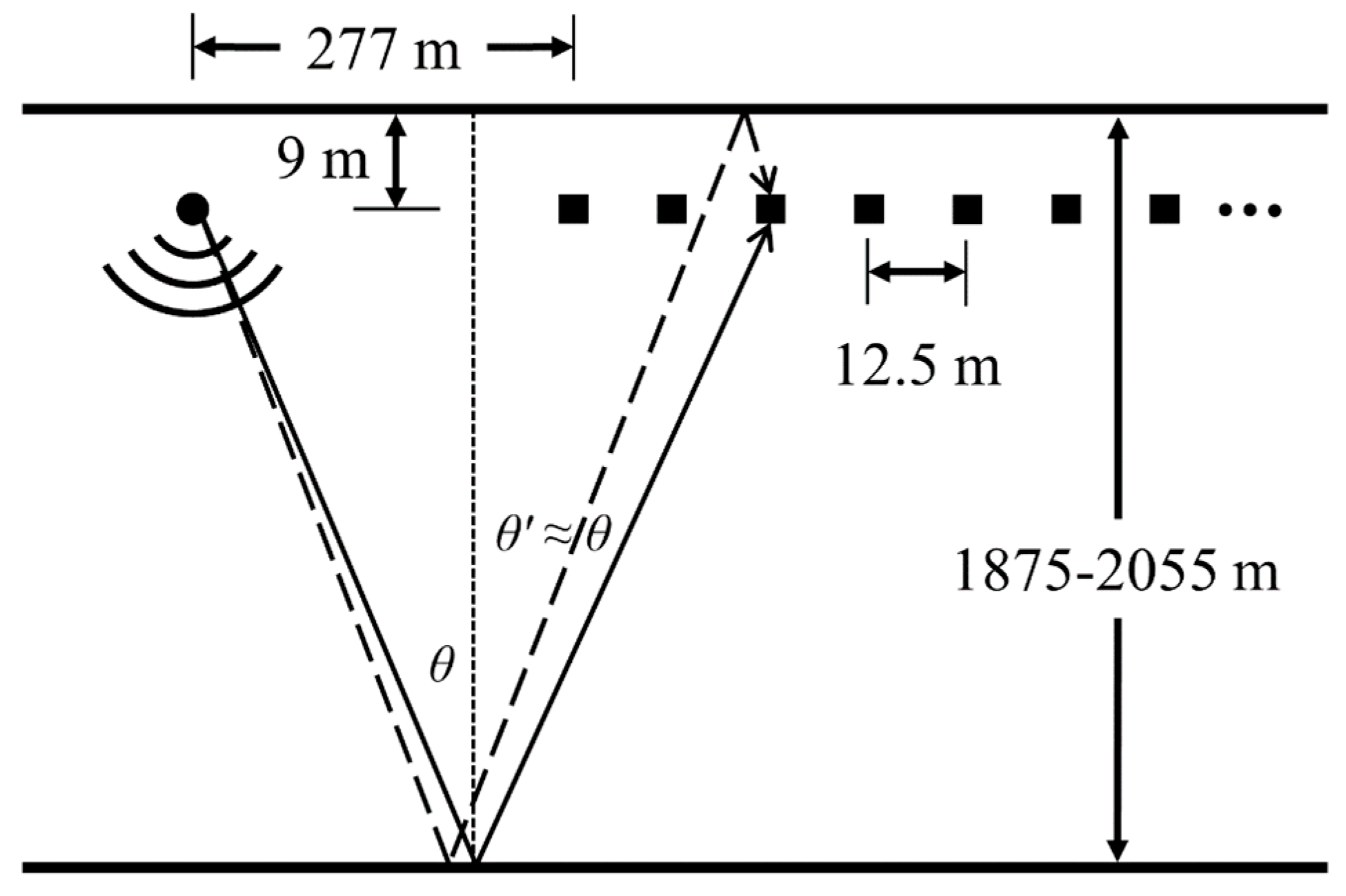
2.4. COAST 2012 Experiment
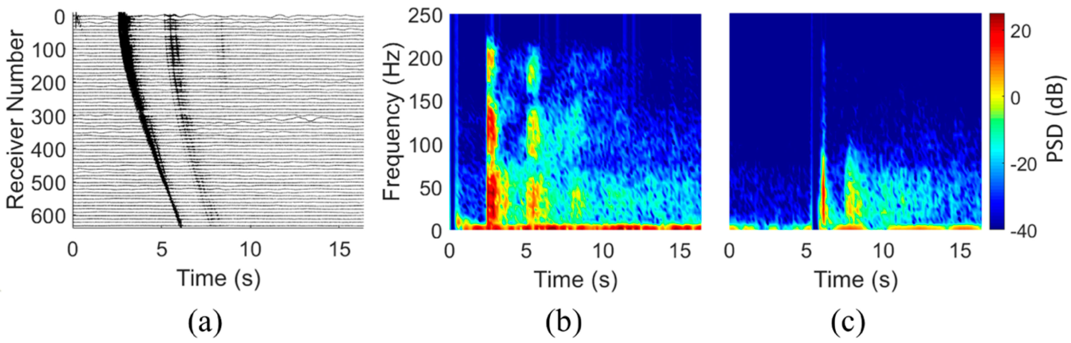
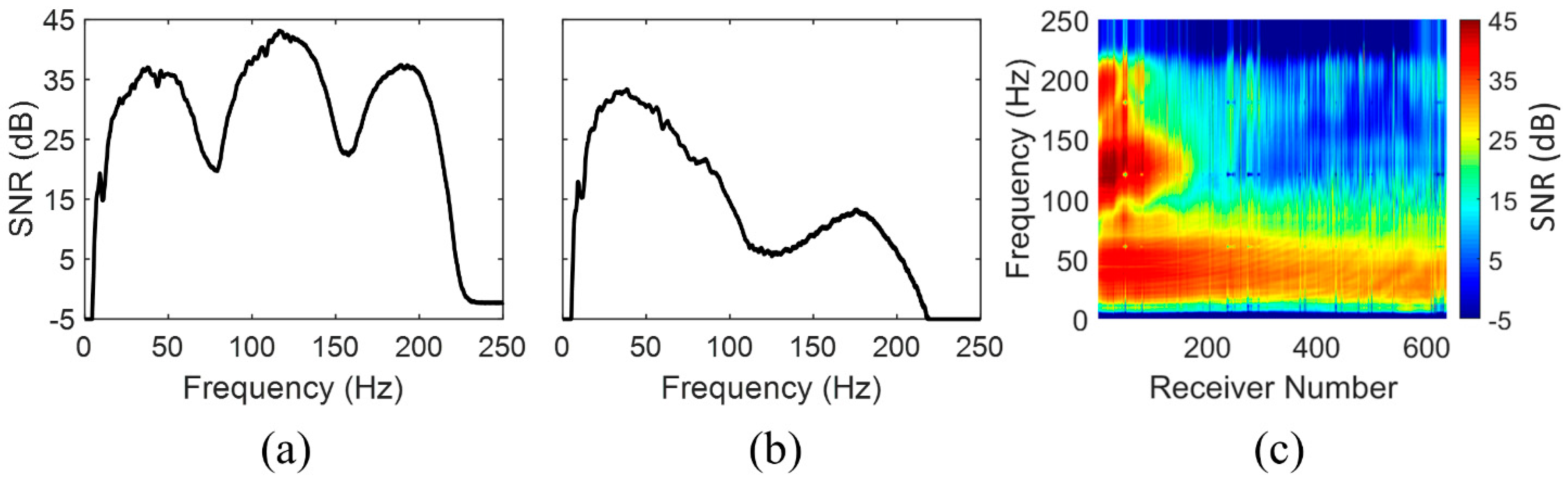
3. Results
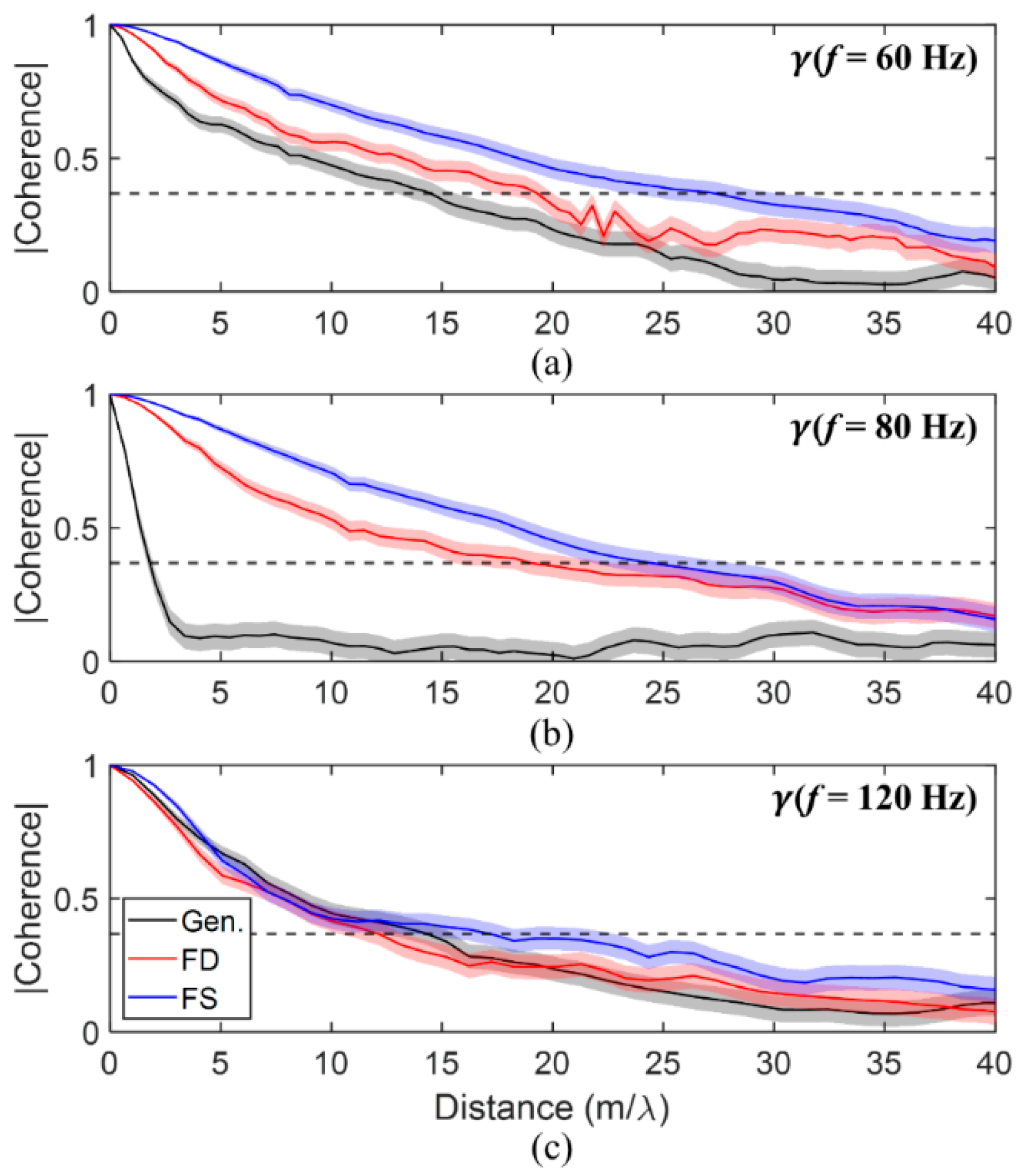
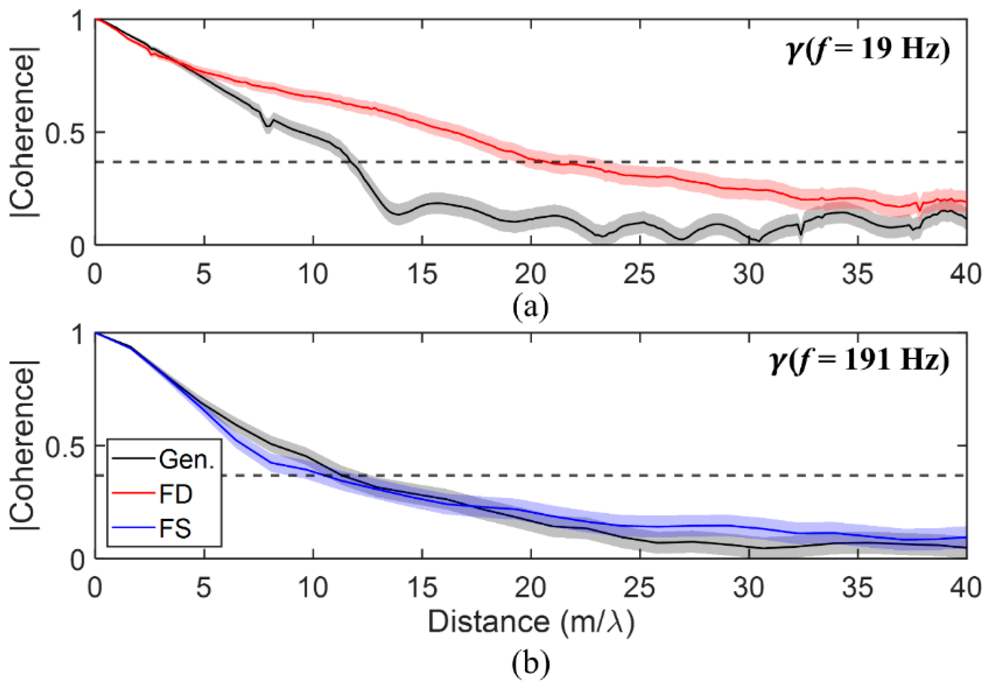
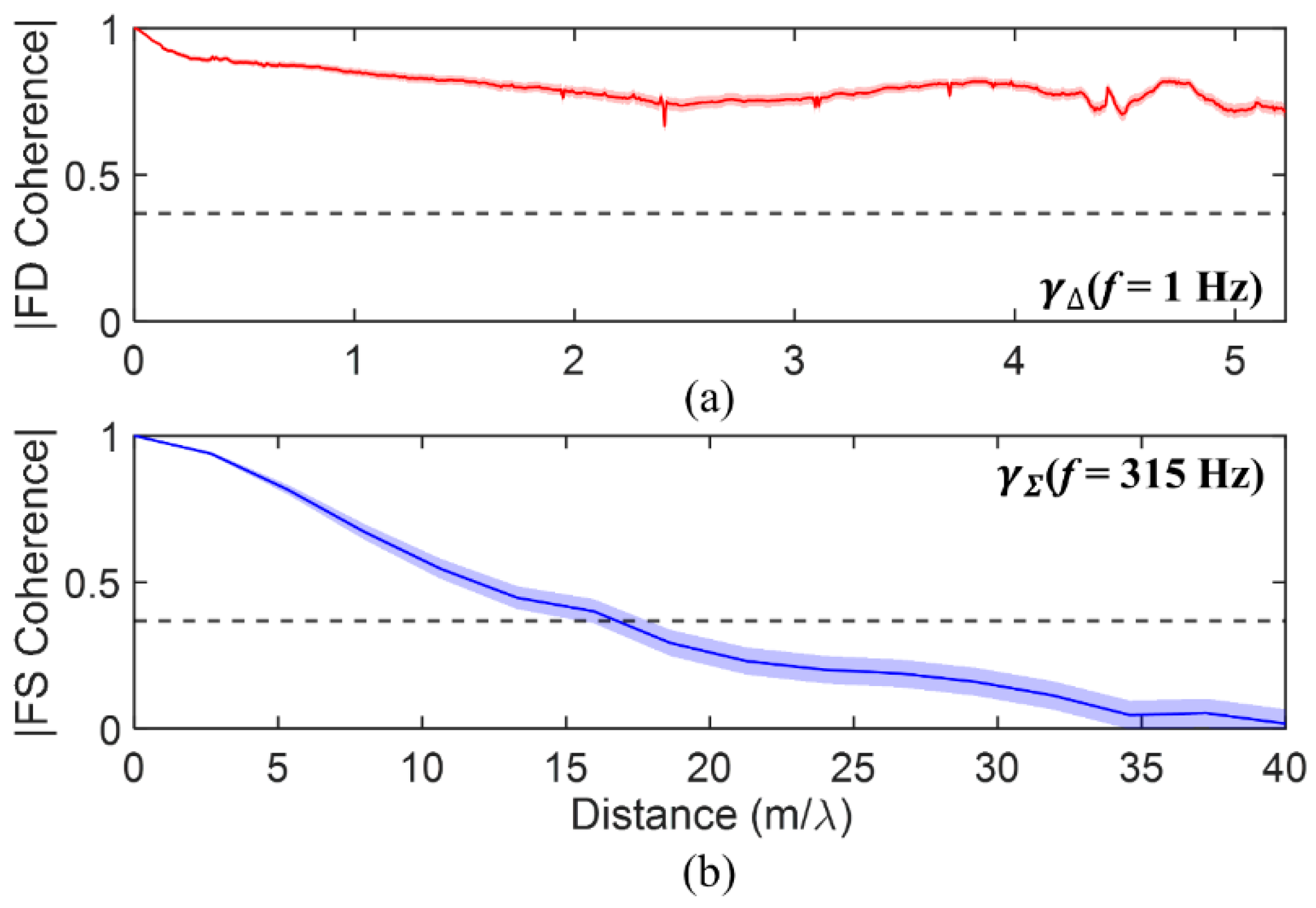
3.1. Coherence
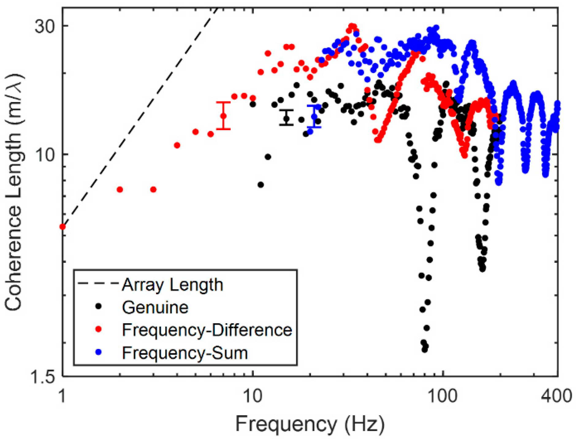
3.2. Coherence Length
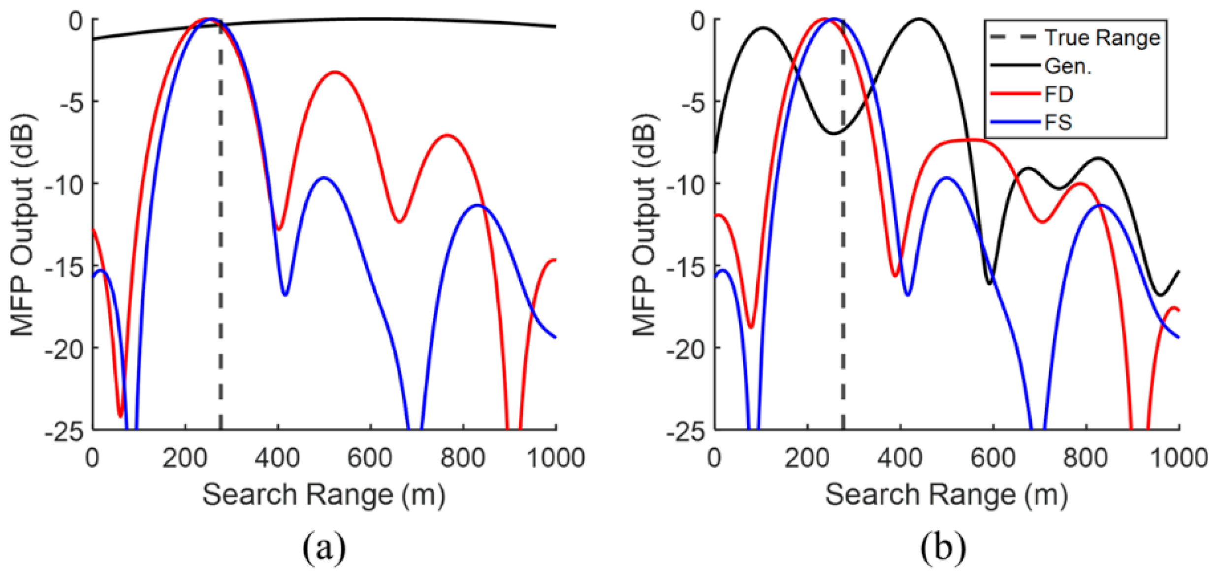
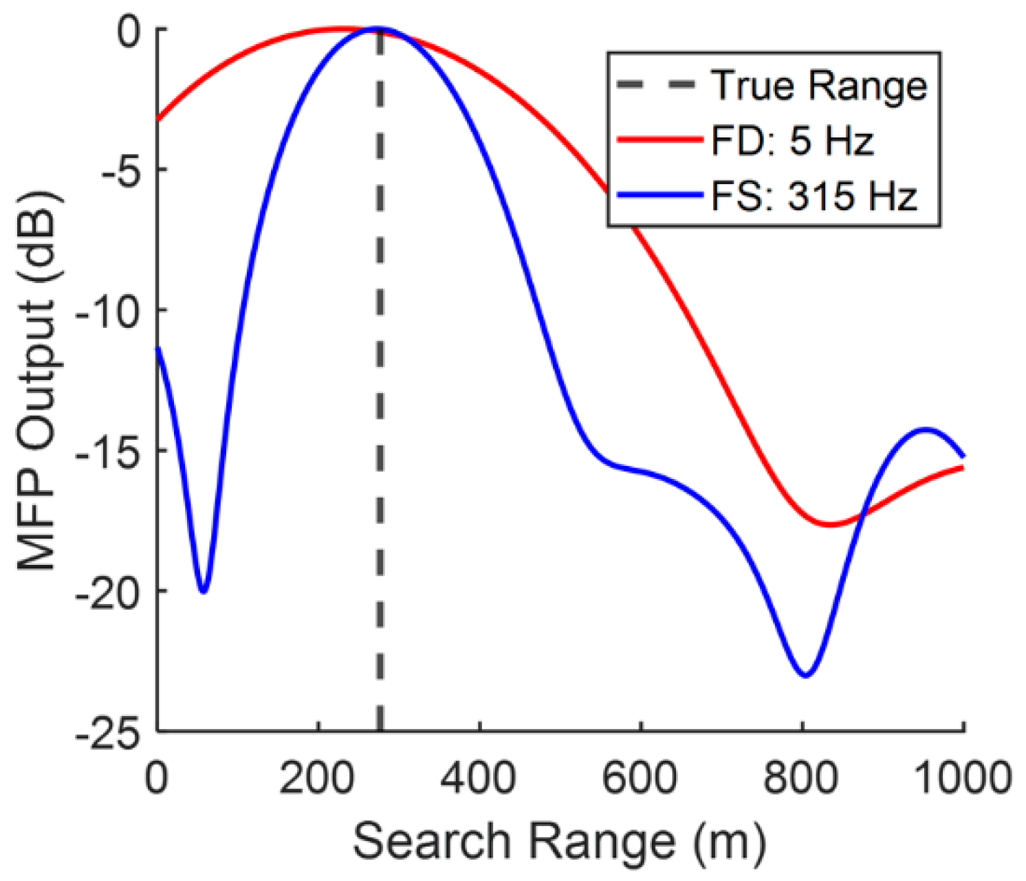
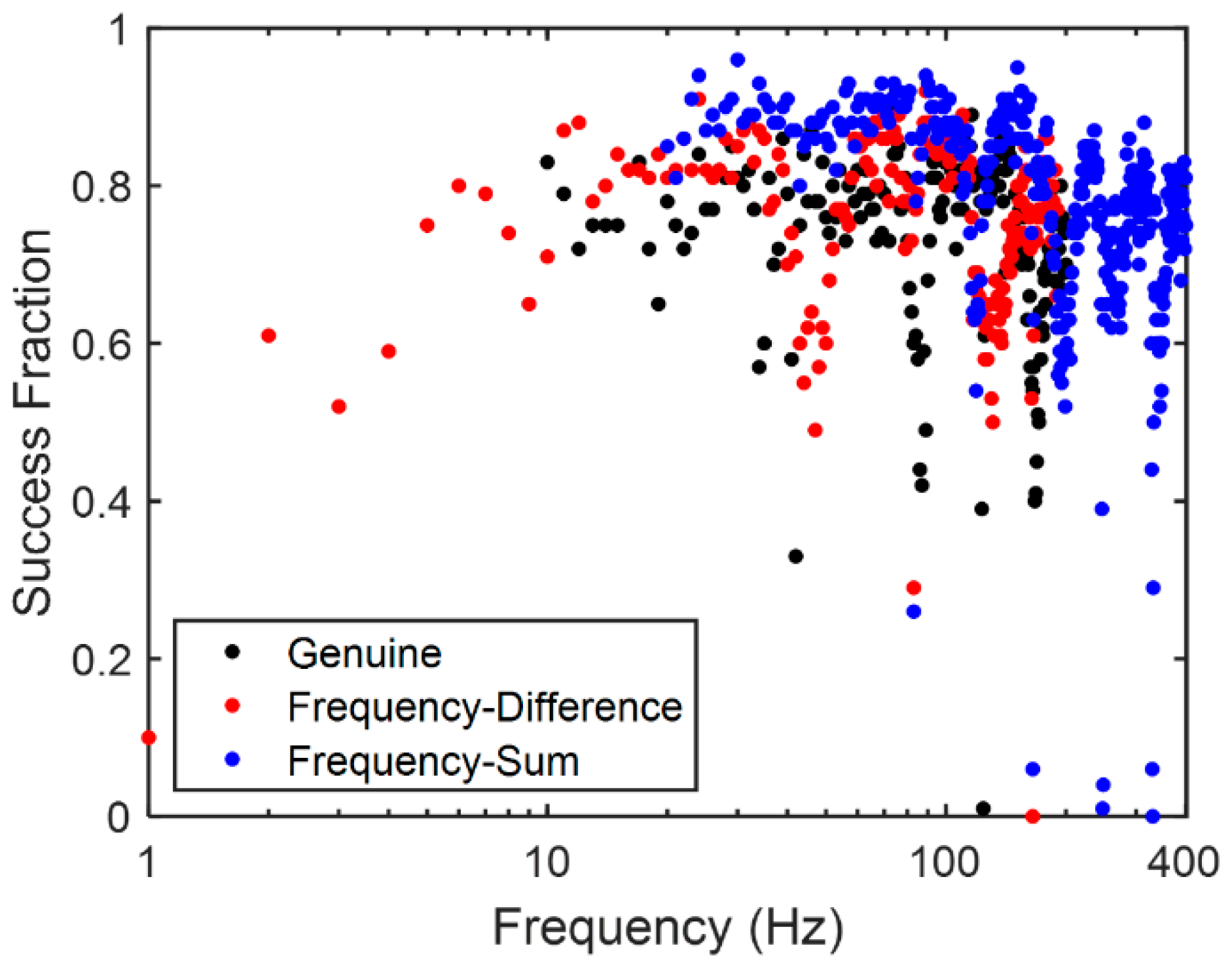
3.3. Extension to Matched-Field Processing
4. Discussion
Author Contributions
Funding
Institutional Review Board Statement
Informed Consent Statement
Data Availability Statement
Acknowledgments
Conflicts of Interest
References
- Urick, R.J. Principles of Underwater Sound, 3rd ed.; McGraw-Hill: New York, NY, USA, 1983. [Google Scholar]
- Heaney, K.D. Shallow Water Narrowband Coherence Measurements in the Florida Strait. J. Acoust. Soc. Am. 2011, 129, 2026–2041. [Google Scholar] [CrossRef] [PubMed]
- Carey, W.M.; Moseley, W.B. Space-Time Processing Environmental-Acoustic Effects. IEEE J. Ocean. Eng. 1991, 16, 285–301. [Google Scholar] [CrossRef]
- Carey, W.M. Determination of Signal Coherence Length Based on Signal Coherence and Gain Measurements in Deep and Shallow Water. J. Acoust. Soc. Am. 1998, 104, 831–837. [Google Scholar] [CrossRef]
- Cox, H. Line Array Performance When the Signal Coherence Is Spatially Dependent. J. Acoust. Soc. Am. 1973, 54, 1743–1746. [Google Scholar] [CrossRef]
- Morgan, D.R.; Smith, T.M. Coherence Effects on the Detection Performance of Quadratic Array Processors, with Applications to Large-Array Matched-Field Beamforming. J. Acoust. Soc. Am. 1990, 87, 737–747. [Google Scholar] [CrossRef]
- Baggeroer, A.B.; Kuperman, W.A.; Mikhalevsky, P.N. An Overview of Matched Field Methods in Ocean Acoustics. IEEE J. Ocean. Eng. 1993, 18, 401–424. [Google Scholar] [CrossRef]
- Rolt, K.D.; Abbot, P.A. Littoral Coherence Limitations on Acoustic Arrays. In Acoustical Imaging; Lees, S., Ferrari, L.A., Eds.; Springer: Boston, MA, USA, 1997; pp. 537–542. [Google Scholar]
- Wan, L.; Zhou, J.X.; Rogers, P.H.; Knobles, D.P. Spatial Coherence Measurements from Two L-Shape Arrays in Shallow Water. Acoust. Phys. 2009, 55, 383–392. [Google Scholar] [CrossRef]
- Finette, S.; Oba, R. Horizontal Array Beamforming in an Azimuthally Anisotropic Internal Wave Field. J. Acoust. Soc. Am. 2003, 114, 131–144. [Google Scholar] [CrossRef]
- Duda, T.F.; Collis, J.M.; Lin, Y.-T.; Newhall, A.E.; Lynch, J.F.; DeFerrari, H.A. Horizontal Coherence of Low-Frequency Fixed-Path Sound in a Continental Shelf Region with Internal-Wave Activity. J. Acoust. Soc. Am. 2012, 131, 1782–1797. [Google Scholar] [CrossRef]
- Lunkov, A.A.; Petnikov, V.G. The Coherence of Low-Frequency Sound in Shallow Water in the Presence of Internal Waves. Acoust. Phys. 2014, 60, 61–71. [Google Scholar] [CrossRef]
- Gorodetskaya, E.Y.; Malekhanov, A.I.; Sazontov, A.G.; Vdovicheva, N.K. Deep-Water Acoustic Coherence at Long Ranges: Theoretical Prediction and Effects on Large-Array Signal Processing. IEEE J. Oceanic Eng. 1999, 24, 156–171. [Google Scholar] [CrossRef]
- Andrew, R.K.; Howe, B.M.; Mercer, J.A. Transverse Horizontal Spatial Coherence of Deep Arrivals at Megameter Ranges. J. Acoust. Soc. Am. 2005, 117, 1511–1526. [Google Scholar] [CrossRef]
- Dowling, D.R.; Jackson, D.R. Coherence of Acoustic Scattering from a Dynamic Rough Surface. J. Acoust. Soc. Am. 1993, 93, 3149–3157. [Google Scholar] [CrossRef]
- Dahl, P.H. Forward Scattering from the Sea Surface and the van Cittert–Zernike Theorem. J. Acoust. Soc. Am. 2004, 115, 589–599. [Google Scholar] [CrossRef]
- Dahl, P.H. Observations and Modeling of Angular Compression and Vertical Spatial Coherence in Sea Surface Forward Scattering. J. Acoust. Soc. Am. 2010, 127, 96–103. [Google Scholar] [CrossRef]
- Berkson, J.M. Measurements of Coherence of Sound Reflected from Ocean Sediments. J. Acoust. Soc. Am. 1980, 68, 1436–1441. [Google Scholar] [CrossRef]
- Brown, D.C.; Brownstead, C.F.; Lyons, A.P.; Gabrielson, T.B. Measurements of Two-Dimensional Spatial Coher-ence of Normal-Incidence Seafloor Scattering. J. Acoust. Soc. Am. 2018, 144, 2095–2108. [Google Scholar] [CrossRef]
- Worthmann, B.M.; Dowling, D.R. The Frequency-Difference and Frequency-Sum Acoustic-Field Autoproducts. J. Acoust. Soc. Am. 2017, 141, 4579–4590. [Google Scholar] [CrossRef]
- Lipa, J.E.; Worthmann, B.M.; Dowling, D.R. Measurement of Autoproduct Fields in a Lloyd’s Mirror Environment. J. Acoust. Soc. Am. 2018, 143, 2419–2427. [Google Scholar] [CrossRef] [PubMed]
- Abadi, S.H.; Song, H.C.; Dowling, D.R. Broadband Sparse-Array Blind Deconvolution Using Frequen-cy-Difference Beamforming. J. Acoust. Soc. Am. 2012, 132, 3018–3029. [Google Scholar] [CrossRef] [Green Version]
- Abadi, S.H.; van Overloop, M.J.; Dowling, D.R. Frequency-Sum Beamforming in an Inhomogeneous Environment. In Proceedings of the Meetings on Acoustics ICA2013, Montreal, QC, Canada, 2–7 June 2013; Volume 19, p. 055080. [Google Scholar]
- Douglass, A.S.; Song, H.C.; Dowling, D.R. Performance Comparisons of Frequency-Difference and Conventional Beamforming. J. Acoust. Soc. Am. 2017, 142, 1663–1673. [Google Scholar] [CrossRef] [PubMed]
- Abadi, S.H.; Haworth, K.J.; Mercado-Shekhar, K.P.; Dowling, D.R. Frequency-Sum Beamforming for Passive Cav-itation Imaging. J. Acoust. Soc. Am. 2018, 144, 198–209. [Google Scholar] [CrossRef] [PubMed]
- Worthmann, B.M.; Song, H.C.; Dowling, D.R. High Frequency Source Localization in a Shallow Ocean Sound Channel Using Frequency Difference Matched Field Processing. J. Acoust. Soc. Am. 2015, 138, 3549–3562. [Google Scholar] [CrossRef] [PubMed]
- Worthmann, B.M.; Song, H.C.; Dowling, D.R. Adaptive Frequency-Difference Matched Field Processing for High Frequency Source Localization in a Noisy Shallow Ocean. J. Acoust. Soc. Am. 2017, 141, 543–556. [Google Scholar] [CrossRef]
- Geroski, D.J.; Dowling, D.R. Long-Range Frequency-Difference Source Localization in the Philippine Sea. J. Acoust. Soc. Am. 2019, 146, 4727–4739. [Google Scholar] [CrossRef] [PubMed]
- Holbrook, S.; Kent, G.; Keranen, K.; Johnson, P.; Trehu, A.; Tobin, H.; Caplan-Auerbach, J.; Beeson, J. COAST: Cascadia Open-Access Seismic Transects. In Proceedings of the AGU Fall Meeting Abstracts 2012, San Francisco, CA, USA, 3–7 December 2012; Volume 2012, pp. 11–12. [Google Scholar]
- Carter, G.C.; Knapp, C.H.; Nuttall, A.H. Statistics of the Estimate of the Magnitude-Coherence Function. IEEE Trans Audio Electroacoust. 1973, 21, 388–389. [Google Scholar] [CrossRef]
- Dowling, D.R. Revealing Hidden Information with Quadratic Products of Acoustic Field Amplitudes. Phys. Rev. Fluids 2018, 3, 110506. [Google Scholar] [CrossRef]
- Bendat, J.S.; Piersol, A.G. Engineering Applications of Correlation and Spectral Analysis; Wiley and Sons: New York, NY, USA, 1980. [Google Scholar]
- Carter, G.C. Coherence and Time Delay Estimation. Proc. IEEE 1987, 75, 236–255. [Google Scholar] [CrossRef]
- Wang, S.Y.; Tang, M.X. Exact Confidence Interval for Magnitude-Squared Coherence Estimates. IEEE Signal Process. Lett. 2004, 11, 326–329. [Google Scholar] [CrossRef]
- Zoubir, A.M. On Confidence Intervals for the Coherence Function. In Proceedings of the ICASSP, IEEE International Conference Acoustics, Speech, and Signal Process, Philadelphia, PA, USA, 23 March 2005; Volume 4. [Google Scholar]
- Bucker, H.P. Use of Calculated Sound Fields and Matched-Field Detection to Locate Sound Sources in Shallow Water. J. Acoust. Soc. Am. 1976, 59, 368–373. [Google Scholar] [CrossRef]
- Jensen, F.B.; Kuperman, W.A.; Porter, M.B.; Schmidt, H. Computational Ocean Acoustics, 2nd ed.; Springer: New York, NY, USA, 2011. [Google Scholar]
- Hotkani, M.M.; Bousquet, J.F.; Seyedin, S.A.; Martin, B.; Malekshahi, E. Underwater Target Localization Using Opportunistic Ship Noise Recorded on a Compact Hydrophone Array. Acoustics 2021, 3, 611–629. [Google Scholar] [CrossRef]
- Diebold, J.B.; Tolstoy, M.; Doermann, L.; Nooner, S.L.; Webb, S.C.; Crone, T.J. R/V Marcus G. Langseth Seismic Source: Modeling and Calibration. Geochem. Geophys. Geosyst. 2010, 11, Q12012. [Google Scholar] [CrossRef]
- Abadi, S.H.; Freneau, E. Short-Range Propagation Characteristics of Airgun Pulses during Marine Seismic Reflection Surveys. J. Acoust. Soc. Am. 2019, 146, 2430–2442. [Google Scholar] [CrossRef] [PubMed]
- Tolstoy, M.; Diebold, J.; Doermann, L.; Nooner, S.; Webb, S.C.; Bohnenstiehl, D.R.; Crone, T.J.; Holmes, R.C. Broadband Calibration of the R/V Marcus G. Langseth Four-String Seismic Sources. Geochem. Geophys. Geosyst. 2009, 10, Q08011. [Google Scholar] [CrossRef]
- Taylor, J.R. An Introduction to Error Analysis, 2nd ed.; University Science Books: Sausalito, CA, USA, 1997. [Google Scholar]
- Geroski, D.J.; Dowling, D.R. Robust Long-Range Source Localization in the Deep Ocean Using Phase-Only Matched Autoproduct Processing. J. Acoust. Soc. Am. 2021, 150, 171–182. [Google Scholar] [CrossRef] [PubMed]


| Reference | Frequency (Hz) | Source–Receiver Range(s) (km) | Water Column Depth | Notes | |
|---|---|---|---|---|---|
| [11] | 7–25 | 100 | 19 | 80 m | 21-day time scale |
| 7–40 | 200 | 19 | 80 m | <3-h averaging | |
| 10–15 | 224 | 30 | 80 m | Studied internal waves | |
| 10–15 | 400 | 30 | 80 m | HLA—465 m | |
| [4] * | 94–450 | 400 | 137–963 | Deep Ocean | Up to 1200 m sensor separation |
| 60–127 | 323; 337 | 300–800 | Deep Ocean | Moving array, 640 m aperture | |
| 31–234 | 300–600 | 500 | 1.6–4 km | Collection of deep ocean basin results | |
| 10–54 | 200–800 | 4–100 | 65-1000 m | Collection of shallow water experiments | |
| COAST 2012 | 2–18 | 10–200 | 0.3–8 | 1900 m | 8 km aperture |
| 5–30 | 0.3–8 | 1900 m | 12.5 m element spacing | ||
| 8–30 | 0.3–8 | 1900 m | 6-h time scale |
Publisher’s Note: MDPI stays neutral with regard to jurisdictional claims in published maps and institutional affiliations. |
© 2022 by the authors. Licensee MDPI, Basel, Switzerland. This article is an open access article distributed under the terms and conditions of the Creative Commons Attribution (CC BY) license (https://creativecommons.org/licenses/by/4.0/).
Share and Cite
Joslyn, N.J.; Douglass, A.S.; Dowling, D.R. Spatial Coherence Comparisons between the Acoustic Field and Its Frequency-Difference and Frequency-Sum Autoproducts in the Ocean. Acoustics 2022, 4, 764-782. https://doi.org/10.3390/acoustics4030046
Joslyn NJ, Douglass AS, Dowling DR. Spatial Coherence Comparisons between the Acoustic Field and Its Frequency-Difference and Frequency-Sum Autoproducts in the Ocean. Acoustics. 2022; 4(3):764-782. https://doi.org/10.3390/acoustics4030046
Chicago/Turabian StyleJoslyn, Nicholas J., Alexander S. Douglass, and David R. Dowling. 2022. "Spatial Coherence Comparisons between the Acoustic Field and Its Frequency-Difference and Frequency-Sum Autoproducts in the Ocean" Acoustics 4, no. 3: 764-782. https://doi.org/10.3390/acoustics4030046