

The Influence of Listeners’ Mood on Equalization-Based Listening Experience


Department of Information Engineering, Università Politecnica delle Marche, 60131 Ancona, Italy
*
Author to whom correspondence should be addressed.
Acoustics 2022, 4(3), 746-763; https://doi.org/10.3390/acoustics4030045
Submission received: 12 July 2022
/
Revised: 19 August 2022
/
Accepted: 28 August 2022
/
Published: 1 September 2022
(This article belongs to the Special Issue Human's Psychological and Physiological Responses to Sound Environment)
Abstract
:Using equalization to improve sound listening experience is a well-established topic among the audio society. Finding a general equalization curve is a difficult task because of spectral content influenced by the reproduction system (loudspeakers and room environment) and personal preference diversity. Listeners’ mood is said to be a factor that affects the individual equalization preference. In this study, the effect of a listener’s mood on equalization preference is tried to be investigated. Starting from an experiment with fifty-two listeners, considering five predefined equalization curves and a database of ten music excerpts, the relationship between listeners’ mood and preferred sound equalization has been studied. The main findings of this study showed that the “High-frequency boosting” equalization was the most preferred among participants. However, the “High-frequency boosting” preference of low-aroused people was slightly lower than the high aroused listeners, increasing the preference of the “Low-frequency boosting”.
1. Introduction
Music is inextricably linked to emotions in a dual way: the emotion recognized in music (perceived emotion) and the emotion that listeners feel while listening to music (induced emotion) [1]. A lot of progress has been observed in the music emotion recognition (MER) field, where advanced predicting models are used with the aim of automatically categorizing the perceived emotion, using the rhythm and tempo of the song as remarkable indicators [2]. Moreover, previous research has shown that music induces changes in the human autonomic nervous system, which controls human emotional arousal (i.e., induced emotion) [3]. In particular, a significant part of the reported emotions of the listeners can be predicted from a set of six psychoacoustic features of music, namely loudness, pitch level, pitch contour, tempo, texture, and sharpness [4]. Perceived and induced emotions are usually identical; however, there are cases in which they differ from each other [5]. Human emotional response to music stimuli is not so straightforward, as a range of underlying psychological mechanisms mediates, such as brain stem reflex, contagion, episodic memory, and musical expectancy [6]. In general, recognizing the perceived emotion is easier than detecting the induced emotion, as the former can occur from analyzing the musical signal features while the latter depends on a variety of factors, such as personal taste in music, memories of the listener, etc. From the above considerations, it becomes clear that defining and controlling the effect of music on humans, by feature extraction techniques, is a challenging procedure.
Apart from emotion, mood is a psychological term used in the music industry. These two terms are usually used interchangeably; however, their difference is theoretically clearly defined: emotion corresponds to a brief but intense affective reaction, while mood corresponds to an unfocused low intensity state [7]. While an emotion is a short-lasting feeling caused by an event, such as brief music content, mood is the long-lasting feeling that either can be recognized in the song (i.e., mood of music), or can characterize the emotional state of an individual (i.e., mood of the listener). Similarly to the distinction between perceived and induced emotion, the distinction between the perceived mood (i.e., the mood recognized in the music) and the induced mood (i.e., the mood of the listener while listening to music) is not always straightforward.
In a general sense, the identification of an individual’s emotion and mood is a difficult task. A commonly used evaluation method is a self-reporting procedure, that can use alternatively a categorical or a dimensional model. In the categorical model, the participant is asked to choose among a set of predefined words, while in the dimensional model, the words that describe the listener’s mood are arranged in a two-dimensional scheme composed by a vertical arousal axis and a horizontal valence (or pleasure) axis [8]; however, the major problems of the self-reporting method are the different perception of mood descriptors among people and the inability of people to understand and articulate their feelings. In this study, a hybrid model that combines both dimensional and categorical evaluations is used in an attempt to reduce the above two problems. An alternative, promising way for capturing human emotion and mood is by measuring specific human physiological responses. Previous research has shown that electroencephalography (EEG), heart rate variability (HRV), and galvanic skin response (GSR) are some of the most meaningful indicators of participants’ mood and emotion [9,10]; however, the use of these parameters implies a long period of observation, while in this work we have decided to study the immediate impact of sound experience on listeners.
Regarding audio equalization, it is a powerful tool to improve the listening experience [11]. An equalizer is used to adjust the sound level of frequency bands in a way that it meets the personal preference of the listener, so it could be evaluated through subjective analysis. An equalizer can be used either in the music production stage, in which experienced audio engineers equalize songs by means of specialized software, or in home/car stereo systems, or even in mobile smartphones where usually a parametric equalizer is implemented in the form of “Bass”, “Midrange”, and “Treble” knobs. Additionally, equalization is used to improve the performance of sound reproduction systems. A non-ideal audio system (i.e., small loudspeakers and non-linear amplifier) and the room environment characteristics can modify the listening experience, introducing undesired artifacts. In this context, several approaches can be found in the literature for room response equalization (RRE), which are used to improve the quality of the sound reproduction system. For a complete review on RRE, it is possible to refer to [12]. In this study, we focus only on the first type of equalization, which is applied for modifying the audio experience according to personal preference, avoiding the correction of the reproduction system. Future studies will be focused on this scenario.
Another important aspect is the listener’s sound perception, which depends on the human auditory system that incorporates a sound weighting process, known as equal loudness level contour (ELC) [13]. By definition, an equal-loudness contour is a measure of sound pressure level, over the frequency spectrum, for which a listener perceives a constant loudness when presented with pure steady tones. The ELC is not identical for every person, leading to different perception of sound among humans. Apart from the different ELC among humans, the preference on the type of equalization can differ from one listener to another depending on the age, the gender, and the prior listening experience [14]. For example, previous research shows that women tend to prefer the normal treble over artificially boosted bass. This characteristic may be connected to the fact that the female ear canal is generally smaller than the male ear canal [15]. In addition, younger and less experienced listeners tend to prefer more bass and treble [14]. Moreover, the same person presents different ELC for different levels of audio reproduction gain. Towards this idea, in [16] a novel equalization approach is proposed to achieve subjectively constant equalization irrespective of the audio reproduction gain, based on the established perceived loudness model. The above considerations make clear the fact that there is no standard equalization curve that optimizes the listening experience for all human, even for the same song. The question that arises is if a listener’s mood can affect the equalization preference.
The contemporary music industry relies heavily on music recommendation systems, providing the possibility of mood-based music selection. It would be very interesting to be able to modify a song by means of an equalizer based on the perceived mood, by adjusting the timbre features, without changing the rhythm, the melody, and the harmony of the reproduced music. Towards this idea, recent research is focused on mapping an acoustic concept expressed by means of descriptive words (e.g., make the sound more “warm”) to equalizing parameters [17]. In particular, a weighting function algorithm is introduced to discover the relative influence of each frequency band on a descriptive word which characterizes the music mood. Adjusting the timbre (tonal quality) of a sound is a complicated procedure, because there are non-linear relationships between changed equalization settings and the perceived sound quality variation. Moreover, equalization is a context-dependent procedure and this means that the same equalization curve can have different effect on different songs. In an attempt to face these not-so-consistent concepts, descriptive words are suggested to be considered in two different groups: words that have monotonic relationship with parameters, and words with a non-monotonic relationship. In this sense, “brightness” is considered a monotonic descriptor, because the increasing of the treble-to-bass ratio always leads to the increase in “brightness”. On the contrary, “fullness”/“darkness” is considered a non-monotonic descriptor, as the reduction in the treble-to-bass ratio leads to increase the “fullness”/“darkness” until a point, but beyond that, the perceived “fullness”/“darkness” decreases or even the sound quality is degraded [18,19]. Following the above ideas, a perceptual assistant to do equalization is proposed in [20] to adjust the timbres of brightness, darkness, and smoothness in a context-dependent fashion. In addition, the interface “Audealize”, introduced in [21], allows the listener to adjust the equalization settings by selecting descriptive terms in a word map, which consists of word labels for audio effects. As mentioned above, this smart equalization is related to the perceived emotion but there are not clear indices about what is happening to the induced emotion.
As said, music can have an impact on the listener’s mood (i.e., induced feeling) but, at the same time, the current listener’s mood has an effect not only on the music track selection (reference), but also on the spectral features of a song that a listener wants to emphasize (i.e., equalization preference). So far, the field of correlating listeners’ mood and preferred music equalization is not established in the literature, leaving room for research. The novelty of this study lies in the idea of exploring the relation between audio equalization preference and listeners’ arousal and pleasure states.
The paper is organized as follows. In Section 2, the equalization curves and audio dataset used in the experiment, the equipment calibration, and the experimental procedure are presented. In Section 3, the results of the experiments, given by 52 participants for 10 tracks, are presented. Specifically, the equalization preference for the different listener mood states, interpreted in terms of listener’s arousal and pleasure, is analyzed. In Section 4, the conclusions are drawn.
2. Materials and Methods
In the following experiment, listeners were asked to express an equalization preference out of five predefined equalization curves, for ten music excerpts of various music genres. The five equalization curves are described in detail in Section 2.1. The listening tests were conducted through headphones. Audio material was pre-processed to compensate the headphones impulse response, as described in Section 2.2. The experimental music dataset is described in Section 2.3. The experimental procedure is described in Section 2.4.
2.1. Equalization Curves
In this study, five predefined equalization curves, shown in Figure 1, are considered through listening tests. The equalization curves settings are shown in detail in Table 1. Similar curves were used in previous research with the purpose to investigate the impact of personalized equalization preference on music quality, as in [22,23].
The equalization curves are based on shelving filters or parametric equalizer (EQ) filters [24]. Shelving filters are usually in the form of a “Bass” or “Treble” knob in audio reproduction systems. A shelving filter can be either a boost/amplification filter or a cut/attenuation filter. Moreover, it can be either low shelf, resembling a shelf that effectively affects the frequencies in the low-end below the cut-off frequency, or high shelf, resembling a shelf that effectively affects the frequencies in the high-end above the cut-off frequency. The current experiment evaluates a boost “Low shelving” filter and a boost “High shelving” one, depicted in Figure 1 by the blue and the red curves, respectively. Both shelving filters are implemented as a single second-order section (biquad) IIR filter by means of MATLAB Audio Toolbox software. The cut-off frequencies () for the low shelving and the high shelving filter are 2 kHz and 200 Hz, respectively. The gain (G) and slope are 7 dB and 0.75 for both filters.
The “Midrange boost” curve is a psychoacoustic-based equalization curve motivated by the equal loudness contour of the ISO-226 standard [13]. The “Midrange boost” curve differs from the high shelving filter for the presence of a peak at about 3 kHz and a notch at about 8 kHz. It is implemented as a parametric equalizer using three cascaded second-order filters with a specific bandwidth, center frequency, and quality factor. The “Midrange dip” curve is derived by reversing the “Midrange boost” curve. Similarly to the shelving filters, “Midrange boost” and “Midrange dip” were implemented by means of MATLAB Audio Toolbox software, depicted with purple and yellow color, respectively, in Figure 1. The central frequencies of the 3 cascaded parametric EQs (, , ) are 6 kHz, 1.5 kHz, and 8.5 kHz, and the quality factors (, , ) are 0.3, 1 and 0.85, respectively, for both “Midrange boost”and “Midrange dip” curves. The gains of the 3 cascaded parametric EQs (, , ) are 10 dB, dB, and dB for the “Midrange boost” filter and dB, 2 dB and 6 dB for the “Midrange dip” curves. The application of “Midrange boost” may enhance vocal over the instrument, while the application of “Midrange dip” curve may enhance the instrumental components. The “Transparent” case denotes the absence of any equalization. The specific filter parameters are described in detail in Table 1. The equalization filters were applied to each channel of the audio material independently, through time-domain convolution. Equalization of the audio material was applied off-line by means of MATLAB.
2.2. Headphones Calibration
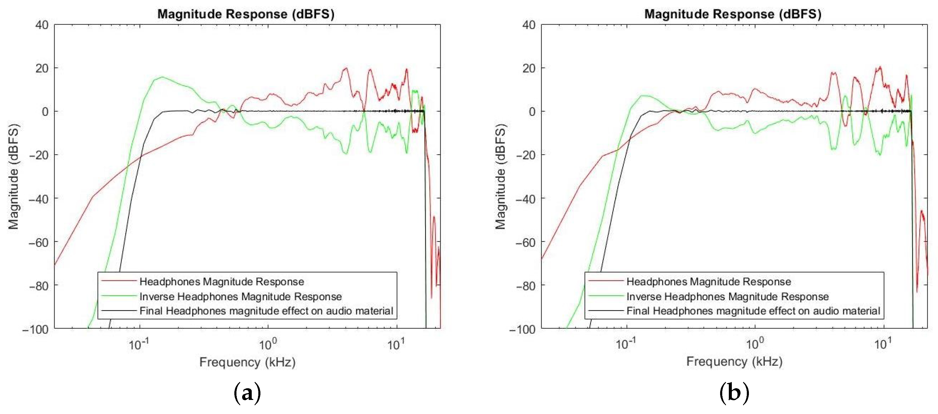
For the audio reproduction, AKG-K52 over-ear closed-back professional headphones were used. The chosen audio dataset was pre-equalized to the inverse headphones impulse response to remove the effect of headphones transfer function during the playback reproduction. The headphone impulse response measurement was acquired through a Head and Torso Simulator (HATS) device, Brüel & Kjær 4128C. The length of the headphone’s impulse response was 2048 samples and the sampling frequency 44.1 kHz. The inverse headphone’s impulse response is a finite response filter (FIR), which was obtained through a fast deconvolution method using frequency dependent regularization [25]. In particular, only frequencies from 100 Hz to 16,500 Hz (frequency range) were inverted with a maximum gain of 8 dB, while frequencies outside this range were damped by 8 dB (gain factor). The specific parameters (i.e., frequency range and gain factor) were selected after a trial and error procedure. The measured curves and the equalization ones are shown in Figure 2, for the left ear (Figure 2a) and for the right ear (Figure 2b). The red curve is the measured headphones frequency response, the green curve is the inverse headphones frequency response, and the black curve is the final magnitude effect of the headphones on the audio material.
2.3. Audio Dataset
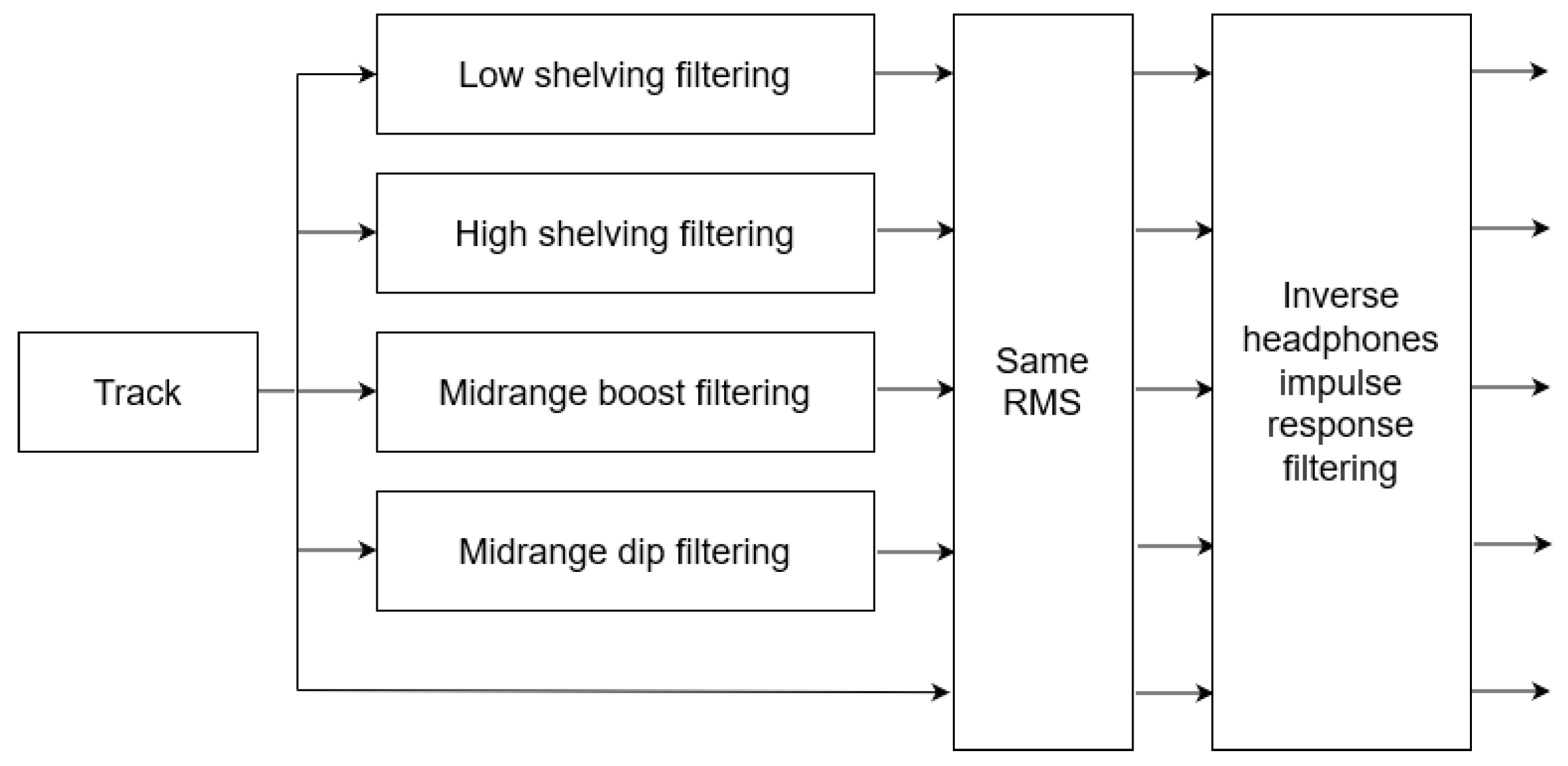
The experimental dataset consisted of 10 songs derived from an online repository of royalty-free and free to download music (stereo.WAV files, with a duration ranging from 20 to 30 s among tracks, 16-bit resolution, and a sampling rate of 44.1 kHz) [26]. The tracks dataset used in the experiment is shown in Table 2. The songs of the specific dataset are created by independent artists, and thus the possibility that a track could be familiar to participants was reduced. Exceptionally, only for classic music a famous Bach concerto was selected, denoted as “Classic 1”. Two tracks for each of the five music genres (namely classic, pop, rock, soul, jazz) were selected to correlate listeners’ mood and equalization preference depending on music genre. Care was taken for selecting excerpts whose spectral features and intensity remained unchanged during their whole duration, while the song quality was of little concern. Moreover, no phrase in the excerpts was interrupted. All 10 excerpts were filtered to the 4 different equalization curves described in Section 2.1. All tracks’ volume, including the original excerpts as well as the equalized version, were adjusted to the same average RMS (root-mean-square) value; thus, no frequency weighting was involved in this procedure. This way, the perceived loudness level did not diverge significantly among the different versions of a song, eliminating any possible biases on the equalization curve preference due to the human tendency towards the louder music, a phenomenon broadly discussed in the literature and the audio engineering society, known as “Loudness War” [27]. This procedure is depicted in Figure 3.
2.4. Implementation
The experiment configuration was web-based and ran on a local server. A large part of the experiment was based on the open-source code of “WebMushra” software tool [28].
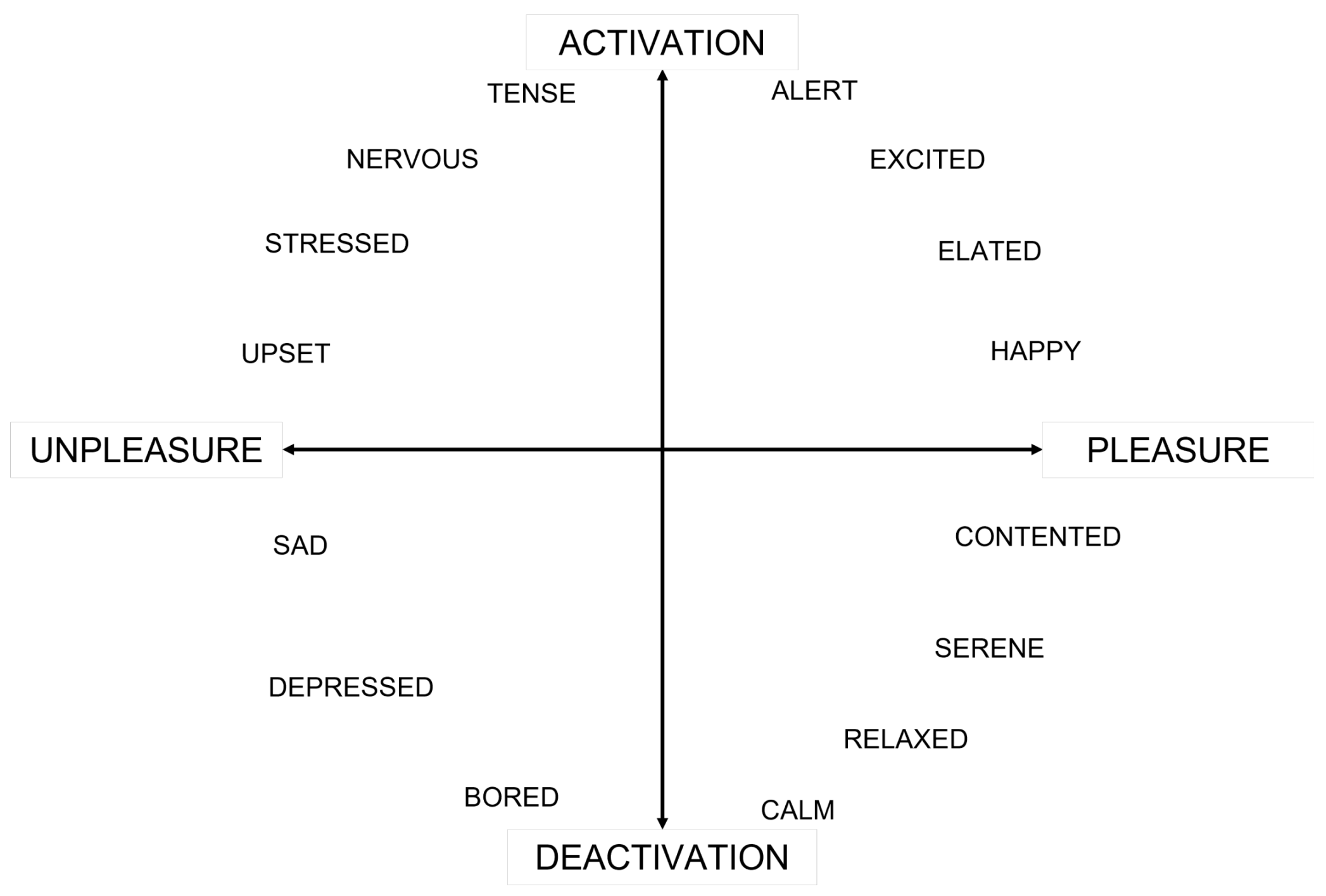
At first, participants were asked to choose the mood descriptor that best described their current mood. A set of descriptors located in specific positions on a two-dimensional model formed by the axes of pleasure/displeasure horizontally, and activation/deactivation vertically in both English and Italian language was available, shown in Figure 4. To avoid language ambiguities between English and Italian, the horizontal axis was orally described as an indicator of good or bad mood, while the vertical axis as an indicator of listener’s energy. The suggestion was to choose a single mood descriptor, but in the case of there being no appropriate single choice, participants were allowed to choose at maximum three of them, and strongly encouraged to take into consideration the position of the mood descriptor in reference to the pleasure (horizontal) and the arousal/activation (vertical) axis.
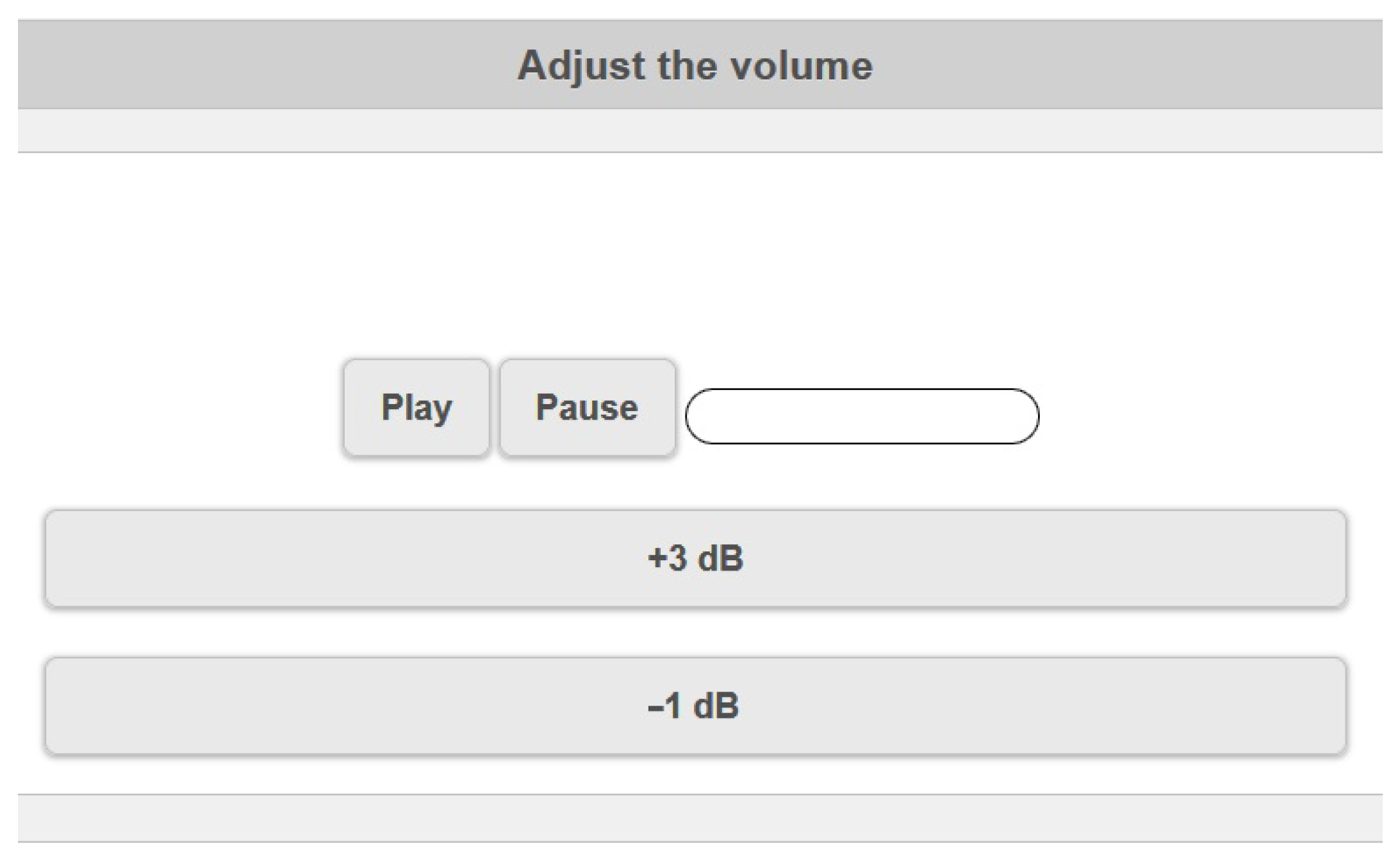
Afterwards, a pure tone air conduction test was conducted to test the audibility thresholds of participants, for specific frequencies. The GUI for a single trial is depicted in Figure 5. The purpose of this procedure was to exclude participants with hearing impairments. The used methodology relied on the recommended procedure of the British Society of Audiology for pure tone audiometry test conduction [29] and a modified Pure Tone Audiometry Technique for Medico-Legal Assessment used in the Royal Liverpool University Hospital [30]. Starting from absolute silence, listeners could turn up the pure tone volume by pressing the “+3 dB ” button (ascending method) until the audible level. Then, listeners started turning down the pure tone volume by pressing the “−1 dB” button (descending method) until the tone was no longer audible. Listeners could repeat this procedure until feeling sure about the threshold decision. The sequence of tone presentation was 1 kHz, 250 Hz, 500 Hz, 4 kHz, and 7 kHz, binaurally, for all participants. An extra 1 kHz tone was presented at the beginning of the pure tone audiometry test, to familiarize participants with the expected threshold level. The above frequencies correspond to the points where the proposed equalization curves of Figure 1 exhibited significant differences; however, this selection does not guarantee the whole-frequency-range hearing normality of a participant. In addition, it should be remarked that, while the threshold audibility test is an accurate enough indicator of hearing impairment, it only provides indices of the frequency analogies (commonly referred to as equal loudness contour) at the sound pressure level where an individual barely recognizes the tone.
The main experimental procedure consisted of the following steps:
- First, for each track of the dataset, participants could listen to and then choose among the 5 types of equalization and, for the selected equalized version of the track, participants set the volume according to their preference. The GUI for a single trial is depicted in Figure 6.
- Finally, for each original, non-equalized track of the dataset, participants evaluated their preference (how much they liked the song context) by means of the Likert scale questionnaire [31], which consists of 4 steps labeled “not at all”, “not a lot”, “much”, and “very much”. The provided guideline was to give importance only to the musical context of the song and to ignore the song quality aspect.
In the first step, in line with Recommendation ITU-R BS.2132-0 “Method for the subjective quality assessment of audible differences of sound systems using multiple stimuli without a given reference” [32], the order of stimuli presentation was randomized from trial to trial to minimize systematic bias effects. Moreover, switching between the 5 differently processed versions of the same track (Cond 1-Cond 5) was instantaneous, without resulting in perceptible temporal shift. The experimenter emphasized to the participants that there is no correct equalization preference and volume level. Instead, participants were encouraged to choose the equalization curve that optimizes their listening experience and the volume they prefer.
The average duration of the test, including the pure tone audiometry test, was 25 min. The experiment was conducted in 3 different rooms, all of which were isolated from external noise, and no visual stimuli could influence participants during the test.
3. Results
The participant sample initially included 36 men and 23 women. Then, seven participants were excluded because of reporting hearing impairments in the pure tone audiometry test. The exclusion criterion was a hearing loss of 30 dB or greater over at least one audiometric frequency. After the exclusion of hearing impaired participants, the panel of participants included 32 men and 20 women between 17 and 58 years old (mean age 26 years old). All of them were Greek or Italian. Further, 22 of them declared that they are playing a musical instrument, while only 7 were audio experts.
3.1. From Categorical Mood Descriptors to Binary Categorization Pleasure/Arousal Analysis
Participants described their mood before the equalization experiment by means of a self-reporting procedure including a set of 15 mood descriptors, as previously discussed and shown in Figure 4. In order to reduce the dimensionality of the relationship analysis, the 15 mood descriptors were interpreted in terms of arousal and pleasure, in accordance to their location on the pleasure/arousal plane. In particular, mood descriptors located above the horizontal axis were interpreted as of “high” arousal and mood descriptors located below the horizontal axis were interpreted as of “low” arousal. Likewise, mood descriptors located left of the vertical axis were interpreted as of “high” pleasure and mood descriptors located right of the vertical axis were interpreted as of “low” pleasure. The mapping of the 15 categorical mood descriptors to arousal and pleasure binary categorization (i.e., “high” and “low”) is described in detail in Table 3. The binarization of mood descriptors is helpful for the statistical analysis and it has already been used in the literature. In [33], a binary categorization of both arousal and valence (i.e., pleasure) has been introduced to reduce the memory requirements of machine learning algorithms used to classify emotions. Participants described their mood choosing from 1 to 3 mood descriptors. The final arousal/pleasure state was decided by the “majority” rule, as described in Table 4. In the event of mood description using two words that correspond to two different arousal/pleasure states (e.g., “high” and “low” arousal, respectively, or “high” and “low” pleasure, respectively), the “majority” rule could not be applied, so these participants were excluded as they did not present a clear arousal/pleasure state. Participant’s allocation over arousal and pleasure states is shown in Table 5.
In the first part of the analysis, equalization preference is analyzed for listeners of high arousal (N = 22) in comparison to listeners of low arousal (N = 23). In the second part of the analysis, equalization preference is analyzed for listeners of high pleasure (N = 37) in comparison to listeners of low pleasure (N = 9). It is worth noting that the number of subjects in the low-pleasure subgroup is less than 25% of the number of subjects in the high-pleasure category, while the arousal-related subgroups have basically the same dimension. The unbalanced distribution of subjects between the low and high-pleasure subgroups limits the dimension of the low-pleasure subgroup under 10 and this can affect the significance of the results, as underlined by the statistical analysis discussed in the following sections.
3.2. Analysis
For the statistical analysis, the five predefined equalization curves were grouped into three categories, according to the frequency region in which they act; therefore, “High-frequency boosting” denotes “High shelving” or “Midrange boost” filtering, as both enhance the higher frequency range. “Low-frequency boosting” denotes “Low shelving” or “Midrange dip” filtering, as both enhance the lower frequency range. “Transparent” denotes no equalization. The ”Midrange boost” curve differs from the “High shelving” for the presence of a peak at about 3 kHz and a notch at about 8 kHz. Similarly, the “Midrange dip” curve differs from the “Low shelving” for the presence of a notch at about 3 kHz and a peak at about 8 kHz. The analysis was conducted without grouping the filtering into the three categories, but keeping the five separated versions. However, several participants declared during the experimental procedure that, for specific tracks, they could not understand the difference between the “Midrange boost” and “High shelving” equalized version of the track. Thus, for the statistical analysis it was decided to group the results derived from “Midrange boost” and “High shelving” together, as both of them have a boosting effect only on the higher frequency range. For consistency reasons, results from “Midrange dip” and “Low shelving” were grouped as well, as both of them have a boosting effect only on the lower frequency range. The relationship between equalization preference and listeners’ mood is analyzed independently for listeners’ arousal and pleasure. Firstly, the results derived from all tracks for high and low-arousal listeners are presented. Following, the results of a genre-based analysis for high and low-arousal listeners are exhibited. Lastly, the results derived from every single track are depicted. The same analysis is conducted for high and low pleasure listeners.
In addition, for a statistical analysis, the Fisher’s exact test [34] was applied in order to check whether the different equalization preferences between high and low moods (arousal or pleasure) were actually significant. It is evaluated by means of the parameter p, that may assume values from 0 to 1. It is important to underline that a p-value less than 0.05 (typically ≤ 0.05) is statistically significant. It indicates strong evidence against the null hypothesis, as there is less than a 5% probability the null is correct (and the results are random) [35].
3.2.1. Influence of Listener’s Arousal on Equalization-Based Listening Experience
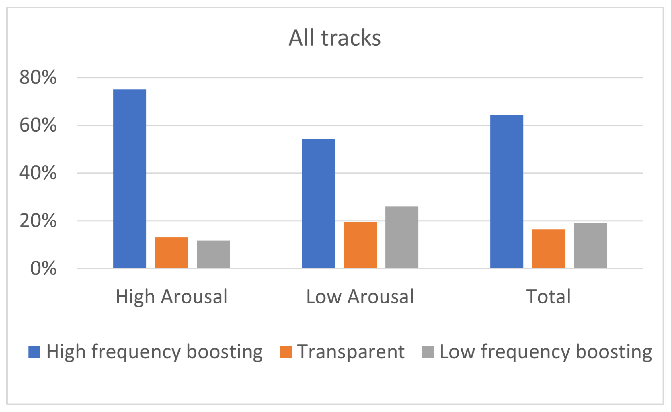
The influence of listeners’ arousal on the equalization preference can be evaluated through the results shown in Figure 7, Figure 8 and Figure 9. “High-frequency boosting” (i.e., “High shelving” and “Midrange boost filtering”) was the predominant equalization curve for listeners of high and low arousal, for all music genres, as indicated by Figure 7 and Figure 8.
Focusing on Figure 7, listeners on high arousal exhibited 75% preference for “High-frequency boosting” (36% for “High shelving” and 39% for “Midrange boost”) while the corresponding percentage for low-arousal listeners was 54% (26% for “High shelving” and 28% for “Midrange boost”). Regarding “Low-frequency boosting” (i.e., “Low shelving” and “Midrange dip filtering”), listeners on high arousal exhibited 12% preference (6% for “Low shelving” and 6% for “Midrange dip”) while listeners on low arousal exhibited 26% preference (10% for “Low shelving” and 16% for “Midrange dip”). Considering “Transparent” filtering (i.e., no equalization), listeners on high arousal exhibited 13% preference while listeners on low arousal 20% preference. These results indicate that the “High-frequency boosting” was always preferred by listeners (both high and low aroused listeners), both of them exhibiting relatively equal preference between “High shelving” and “Midrange boost”; however, the ”High-frequency boosting” preference of low-aroused people was slightly lower than the high-aroused listeners, increasing the preference on the “Low-frequency boosting”. In particular, high-aroused listeners presented equal preference between “Low shelving” and “Midrange dip”, while low-aroused listeners presented higher preference for “Midrange dip” in comparison to “Low shelving”. This means that the equalization that enhances low frequencies is mostly chosen by listeners with low arousal.
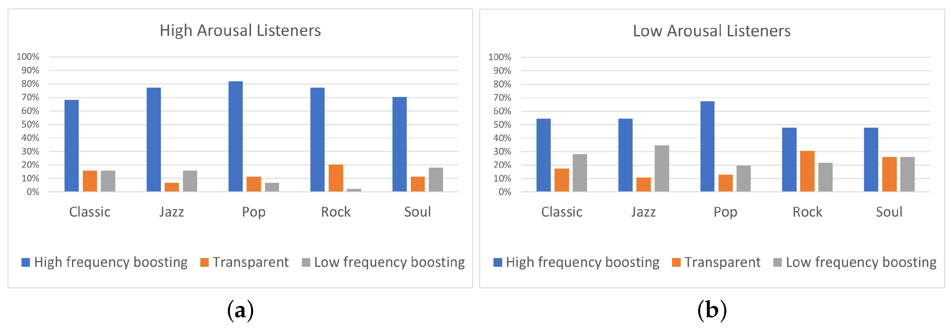
The preference of participants (both high and low aroused ones) towards “High-frequency boosting” is confirmed as well by the genre-based analysis, shown in Figure 8. In this analysis, the 10 tracks of the database were grouped into five categories, based on the genre in which they belong to. Listeners on high arousal exhibited higher percentage of “High-frequency boosting” comparing to listeners on low arousal for all music genres. Especially for Rock and Soul genres, high-aroused participants exhibited 29% higher preference for “High-frequency boosting” comparing to low-aroused participants. Additionally, listeners on low arousal exhibited higher percentage for “Low-frequency boosting” comparing to listeners on high arousal for all the genres. Especially for Jazz and Rock genres, low-aroused participants exhibited more than 19% higher preference for “Low-frequency boosting” comparing to high aroused participants. Thus, the genre-based analysis shown in Figure 8, confirms that, for all the five music genres, more low-aroused participants chose the “Low-frequency boosting” than high-aroused participants. Moreover, listeners on low arousal exhibited more than 10% higher preference for “Transparent” filtering comparing to high arousal listeners for Rock and Soul genres.
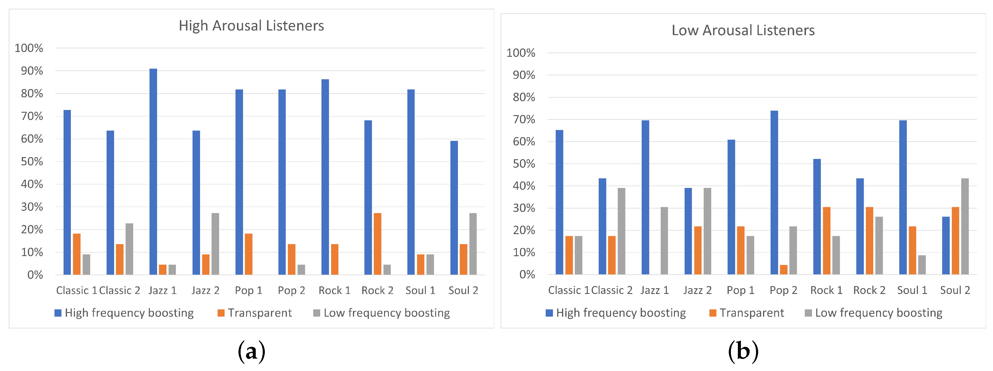
From another perspective, it is interesting to observe the differences presented on equalization preference between high and low-aroused listeners for each track. The Fisher’s exact test was conducted for each track and Table 6 shows the obtained values of the parameter p. A p-value less than 0.05 indicates strong evidence that there is association between listeners’ arousal and the selected equalization curve for the specific track. Focusing on Figure 9, for the Jazz 1 track, listeners on low arousal exhibited 25% higher percentage for “Low-frequency boosting” comparing to listeners of high arousal (). For Rock 1 and Pop 1 tracks, listeners of low arousal exhibited a 17% percentage for “Low-frequency boosting” filtering while none of the highly aroused listeners preferred “Low-frequency boosting” ( and , respectively). Moreover, for the Rock 2 track, listeners on high arousal presented 25% higher percentage for “High-frequency boosting” and 20% lower percentage for “Low-frequency boosting” comparing to low-arousal listeners (). For the Soul 2 track, listeners on high arousal exhibited 60% preference for “High-frequency boosting” while for listeners of low arousal “Low-frequency boosting” was the most preferred equalization curve (). Hence, for the above tracks, it is shown that a lower arousal decreases the agreement between participants without changing the general tendencies (i.e., preference for “High-frequency boosting”). Exceptionally to the general trend, for Soul 2 and Jazz 2 tracks low-aroused listeners presented preference towards “Low-frequency boosting”. The differences on equalization preference, presented between high and low-arousal listeners, were statistically significant only for Jazz 1 and Rock 1 tracks (). On the contrary, Classic 1 track and Soul 1 track presented similar percentages of “High-frequency boosting”, “Low-frequency boosting”, and “Transparent” filtering between high and low-arousal listeners ( and , respectively). Hence, it is shown that, for the specific tracks, listeners’ arousal did not affect the equalization preference. These results indicate that, for specific tracks, listeners’ arousal mostly affected the equalization preference, while for other tracks the equalization preference between high and low-arousal listeners showed similar results. In the former case (i.e., tracks for which listeners’ arousal affected the equalization preference), it is always observed that low-aroused listeners presented higher preference for ”Low-frequency boosting” comparing to high-aroused participants.
3.2.2. Influence of Listener’s Pleasure on Equalization-Based Listening Experience
The influence of listeners’ pleasure on the equalization preference can be evaluated through the results shown in Figure 10, Figure 11 and Figure 12. Despite the fact that the number of participants on high pleasure (N = 37) was substantially bigger in contrast to the low pleasure one (N = 9), the statistical analysis was carried out in the same fashion for both the groups. Figure 10 and Figure 11 indicate that, similarly to the arousal case, “High-frequency boosting” (i.e., “High shelving” and “Midrange boost filtering”) was the predominant equalization curve for listeners of high and low pleasure, for all music genres. As an exception, for the classic genre, listeners on low pleasure presented equal preference for “High-frequency boosting” and “Low frequency boosting”.
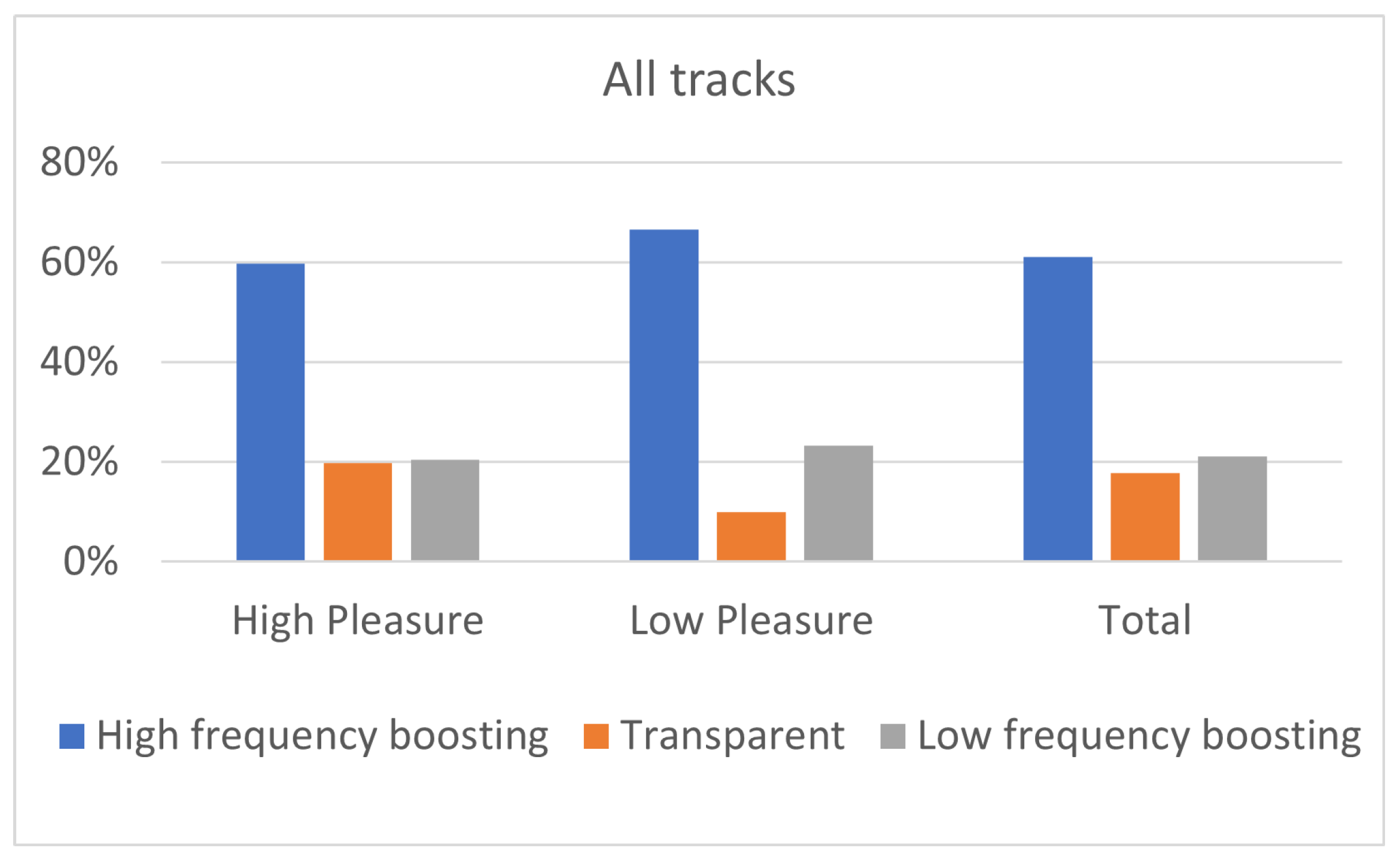
Focusing on Figure 10, listeners on high pleasure exhibited 60% percentage for “High-frequency boosting” (29% for “High shelving” and 31% for “Midrange boost”) while the corresponding percentage for low-pleasure listeners was 66% (33% for “High shelving” and 33% for “Midrange boost”). Regarding “Low-frequency boosting” (i.e., “Low shelving” and “Midrange dip filtering”), listeners on high pleasure exhibited 21% preference (8% for “Low shelving” and 13% for “Midrange dip”) while listeners on low pleasure exhibited 23% preference (13% for “Low shelving” and 10% for “Midrange dip”). Considering “Transparent” filtering (i.e., no equalization), listeners on high pleasure exhibited 20% preference while listeners on low pleasure 10% preference. These results indicate that the “High-frequency boosting” was always preferred by listeners (both high and low pleasured ones), exhibiting relatively equal preference between “High shelving” and “Midrange boost”; however, despite the clear preference of listeners towards “High-frequency filtering”, high-pleasure listeners presented slightly higher preference towards ”Transparent” filtering, comparing to low-pleasure listeners. Regarding “Low-frequency boosting”, high-pleasure listeners presented higher preference for “Midrange dip” in comparison to “Low shelving”, while low-pleasure listeners presented slightly higher preference for “Low shelving” compared to “Midrange dip”.
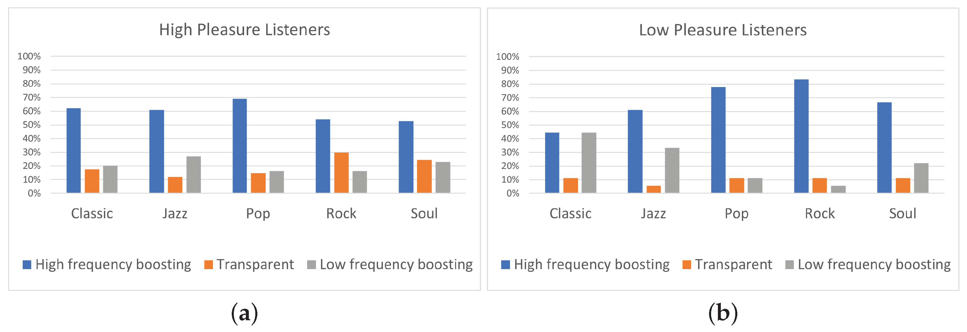
The preference of participants (both high and low-pleasure ones) towards “High-frequency boosting” is confirmed as well by the genre-based analysis; summarized in Figure 11. In this analysis, the 10 tracks of the database were grouped into five categories based on the genre they belong to. Listeners of high pleasure exhibited higher percentage of “Transparent” filtering comparing to listeners of low pleasure, for all music genres. Especially for Rock and Soul genres, highly pleasured participants exhibited more than 13% higher preference for “Transparent” filtering comparing to low-pleasured participants; therefore, it is shown that for all five genres, listeners (both high and low-pleasure ones) presented preference for “High-frequency filtering” and more highly pleasured participants chose the “Transparent” filtering than low-pleasure ones. This result indicates that a “high-pleasure state” seems to drive more participants towards not equalizing at all (“Transparent”). Conversely, a “low-pleasure state” seems to drive more participants towards acting on the equalization. This result appears interesting and could be subjected to different interpretations, which moves beyond the scope of the research herein presented. It should be remarked that during the stimuli presentation, the “transparent” version of the track was “hidden” among the five different versions.
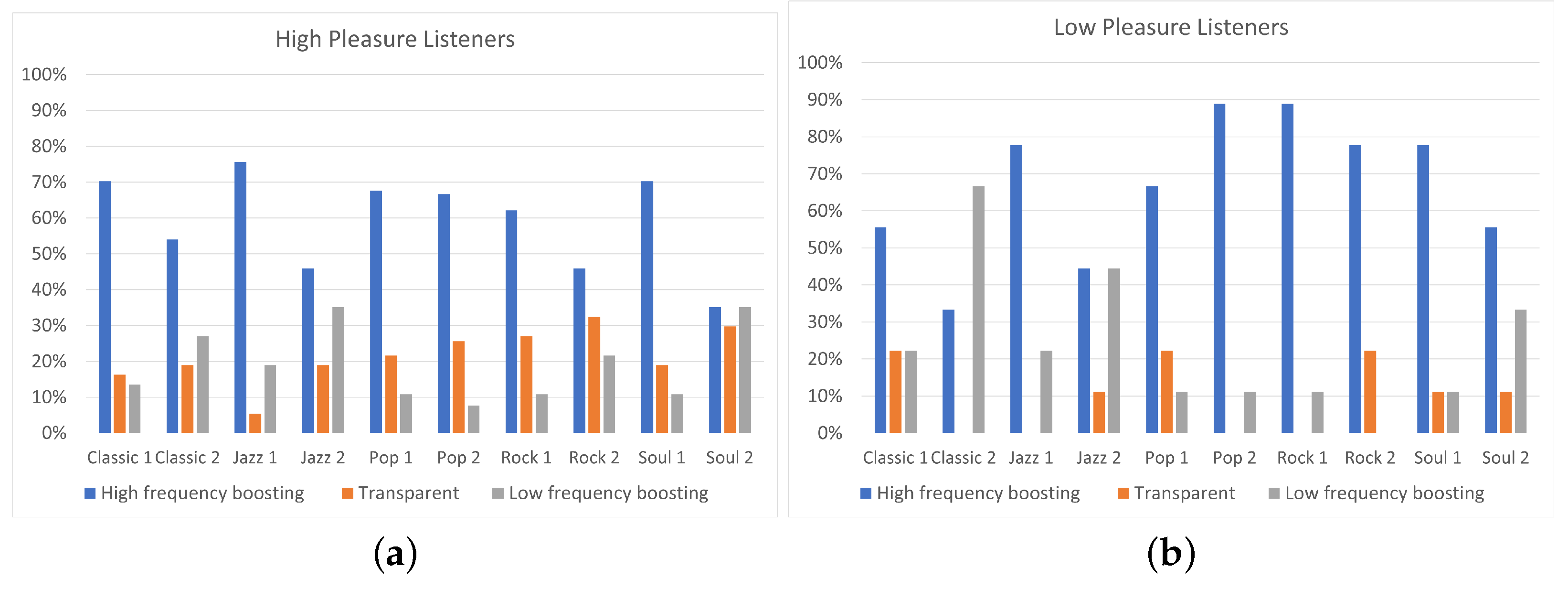
From another perspective, it is interesting to observe, for every single track, the differences presented on equalization preference between high and low-pleasure listeners. In addition, in this case, Fisher’s exact test was conducted for each track and Table 7 shows the obtained values of the parameter p. A p-value less than 0.05 indicates strong evidence that there is association between listeners’ pleasure and the selected equalization curve for the specific track. Focusing on Figure 12, listeners of high pleasure exhibited 19% “Transparent” filtering preference for Classic 2 track, 26% for Pop 2 track, and 27% for Rock 1 track, while none of the low-pleasure listeners preferred “Transparent” filtering for the above tracks (, , and , respectively). Moreover, for the Soul 2 track, listeners on high pleasure exhibited 19% higher percentage for “Transparent” filtering comparing to listeners of low pleasure (). Additionally, for Classic 2 track, listeners of high pleasure exhibited more than 50% preference for “High-frequency boosting”, while listeners of low pleasure presented more than 60% preference for “Low-frequency boosting” (). On the contrary, Classic 1 track and Soul 1 track presented similar percentages of “High-frequency boosting”, “Low-frequency boosting”, and “Transparent” filtering between high and low-pleasure listeners ( and , respectively). Hence, it is shown that, for the specific tracks, the listener’s pleasure did not affect the equalization preference. However, none of the tracks presented statistically significant differences on equalization preference between high and low-pleasure listeners (). These results can be justified by the unbalanced distribution of participants between the low-pleasure and high-pleasure ones, as shown in Table 5.
Comparing the p values obtained for the arousal analysis (Table 6) with the ones shown in the pleasure analysis (Table 7), we can conclude that the differences on equalization preference presented between high and low groups were more significant for arousal, since no significant () values are found in the case of pleasure analysis.
4. Conclusions and Future Work
In this paper, the effect of listeners’ arousal and pleasure on equalization preference was investigated. Participants considered, among a pool of five predefined equalization curves, namely two high-frequency boosting (i.e., “High shelving” and “Midrange boost”), two low-frequency boosting (i.e., “Low shelving” and ”Midrange dip”), and “Transparent” filtering. The dataset consisted of 10 songs, belonging to five different music genres, namely classic, jazz, pop, rock, and soul. Listeners’ arousal and pleasure were classified as high and low. The influence of listeners’ arousal on the equalization preference was analyzed between listeners of high and low arousal. Likewise, the influence of listener pleasure on the equalization preference was analyzed between listeners of high and low pleasure.
Participants’ mood was transcribed by means of 15 predefined mood descriptors located on the pleasure/arousal plane through a self-report procedure, prior to the equalization preference test. Participant’s arousal and pleasure state was decided by, firstly, transforming the categorical mood descriptors to arousal and pleasure binary categorization (“high” and “low”) values, and then, by applying a majority rule over the binary categorization values, as analytically described in Section 3.1. The effect of listeners’ arousal on equalization preference was investigated by analyzing results derived from 45 participants, and the effect of listeners’ pleasure on equalization preference by analyzing results derived from 46 participants.
The results of the experiment indicated that the two high-frequency boosting curves, denoted as a single category labeled “High-frequency boosting”, were the most preferred ones among the five predefined equalization curves, independently of the listener’s arousal and pleasure state. Listeners on high arousal (N = 22) presented higher percentages of “High-frequency boosting” preference, comparing to listeners on low arousal (N = 23). Moreover, low-arousal listeners exhibited higher percentages of ”Low-frequency boosting” filtering choice, comparing to listeners of high arousal. Listeners on high pleasure (N = 37) exhibited higher percentages of ”Transparent” filtering selection, comparing to listeners of low pleasure (N = 9); however, it should be remarked that participants allocation over high and low pleasure states was unbalanced, leading to conclusions that should be further verified by means of additional tests.
Moreover, a statistical analysis has been conducted using Fisher’s exact test showing that the listener’s arousal is a more significant factor for the equalization preference in contrast to pleasure. However, the limited sample dimension does not allow us to obtain a robust indication of the relation between track and pleasure or arousal attitude of a subject. In particular, regarding the pleasure analysis, none of the tracks presented a p-value lower than 0.05. A possible reason for the high p-values is the unbalanced distribution of participants between “high” and “low” pleasure states.
Future research will be oriented to overcome some limitations we found in this study. In particular, regarding the program material, the study included only five music genres, each one represented by only two stimuli. A deeper analysis on different genres with more stimuli would be included for future developments. In addition to this, the small number of participants involved in the study (i.e., 45 for the arousal analysis and 46 for the pleasure analysis) and the unbalanced allocation of participants over the two pleasure states (“high” and “low”), probably led to the obtained statistically non-significant results. In a future work, the participants’ panel could be expanded to eliminate, as well, the impact of personal equalization preference on the results. Furthermore, despite the fact that binary categorization of pleasure/arousal values is commonly used in these kinds of experiments, it is not, to the authors’ best knowledge, part of a validated psychological scale. Moreover, further experiments for the evaluation of listeners’ mood could be conducted using not only self-reporting procedures, but also measuring physiological parameters such as heart rate variability (HRV), galvanic skin response (GSR), and electroencephalography (EEG) to obtain more objective indices of a listener’s mood. This way, several problems affecting the self-reporting procedure, such as difficulties in the awareness of one’s emotions and self-presentation biases (referred to individuals’ tendency to feel uneasy about reporting states that may be seen as undesirable, e.g., depressed mood) would be avoided. Additionally, further research will be conducted on analyzing why equalization preference between high and low arousal/pleasure listeners is different for some tracks and similar for other tracks. A first step towards this concept could be to indicate the specific song’s characteristics that are responsible for this variation.
Author Contributions
Conceptualization, S.S. and S.C.; methodology, N.D. and S.C.; software, N.D.; validation, N.D.; formal analysis, N.D.; investigation, N.D., V.B., S.S. and S.C.; resources, S.S. and S.C.; data curation, N.D.; writing—original draft preparation, N.D. and V.B.; writing—review and editing, N.D., V.B., S.S. and S.C.; visualization, N.D., V.B., S.S. and S.C.; supervision, S.S. and S.C.; project administration, S.C.; funding acquisition, S.C. All authors have read and agreed to the published version of the manuscript.
Funding
This work is supported by Marche Region in implementation of the financial programme POR MARCHE FESR 2014-2020, project “Miracle” (Marche Innovation and Research facilities for Connected and Sustainable Living Environments), CUP B28I19000330007, and partially supported by the financial program DM MiSE 5 Marzo 2018, project “ChAALenge”—F/180016/01-05/X43.
Institutional Review Board Statement
The study was conducted according to the guidelines of the Declaration of Helsinki.
Informed Consent Statement
Informed consent was verbally obtained from all subjects involved in the study.
Data Availability Statement
Not applicable.
Conflicts of Interest
The authors declare no conflict of interest.
References
- Juslin, P.N.; Sloboda, J. Handbook of Music and Emotion: Theory, Research, Applications; Oxford University Press: New York, NY, USA, 2011; pp. 73–97. [Google Scholar]
- Plewa, M.; Kostek, B. A study on correlation between tempo and mood of music. In Proceedings of the 133rd Convention of the Audio Engineering Society, San Francisco, CA, USA, 26–29 October 2012. [Google Scholar]
- Dourou, N.; Poli, A.; Terenzi, A.; Cecchi, S.; Spinsante, S. IoT-Enabled Analysis of Subjective Sound Quality Perception Based on Out-of-Lab Physiological Measurements. In Proceedings of the EAI International Conference on IoT Technologies for HealthCare, online, 24–26 November 2021; Springer: Cham, Switzerland, 2021; pp. 153–165. [Google Scholar]
- Coutinho, E.; Cangelosi, A. Musical emotions: Predicting second-by-second subjective feelings of emotion from low-level psychoacoustic features and physiological measurements. Emotion 2011, 11, 921. [Google Scholar] [CrossRef] [PubMed]
- Song, Y.; Dixon, S.; Pearce, M.T.; Halpern, A.R. Perceived and induced emotion responses to popular music: Categorical and dimensional models. Music Percept. Interdiscip. J. 2016, 33, 472–492. [Google Scholar] [CrossRef]
- Juslin, P.N.; Barradas, G.; Eerola, T. From sound to significance: Exploring the mechanisms underlying emotional reactions to music. Am. J. Psychol. 2015, 128, 281–304. [Google Scholar] [CrossRef] [PubMed]
- Eerola, T. Modeling emotions in music: Advances in conceptual, contextual and validity issues. In Proceedings of the Audio Engineering Society Conference: 53rd International Conference: Semantic Audio, London, UK, 26–29 January 2014. [Google Scholar]
- Russell, J.A. A circumplex model of affect. J. Personal. Soc. Psychol. 1980, 39, 1161. [Google Scholar] [CrossRef]
- Rumsey, F. Quality, emotion, and machines. J. Audio Eng. Soc. 2021, 69, 890–894. [Google Scholar]
- Poli, A.; Brocanelli, A.; Cecchi, S.; Orcioni, S.; Spinsante, S. Preliminary Results of IoT-Enabled EDA-Based Analysis of Physiological Response to Acoustic Stimuli. In IoT Technologies for HealthCare; Goleva, R., Garcia, N.R.D.C., Pires, I.M., Eds.; Springer International Publishing: Cham, Switzerand, 2021; pp. 124–136. [Google Scholar]
- Välimäki, V.; Reiss, J.D. All about audio equalization: Solutions and frontiers. Appl. Sci. 2016, 6, 129. [Google Scholar] [CrossRef]
- Cecchi, S.; Carini, A.; Spors, S. Room response equalization—A review. Appl. Sci. 2017, 8, 16. [Google Scholar] [CrossRef]
- ISO 226:2003; Acoustics—Normal Equal-Loudness-Level Contours. Available online: https://www.iso.org/standard/34222.html (accessed on 12 July 2022).
- Olive, S.; Welti, T. Factors that influence listeners’ preferred bass and treble levels in headphones. J. Audio Eng. Soc. 2015, 139, 9382. [Google Scholar]
- McCown, W.; Keiser, R.; Mulhearn, S.; Williamson, D. The role of personality and gender in preference for exaggerated bass in music. Personal. Individ. Differ. 1997, 23, 543–547. [Google Scholar] [CrossRef]
- Drossos, K.; Floros, A.; Kanellopoulos, N.G. A Loudness-based Adaptive Equalization Technique for Subjectively Improved Sound Reproduction. In Proceedings of the 136th Convention of the Audio Engineering Society, Berlin, Germany, 26–29 April 2014. [Google Scholar]
- Aspinwall, A. Communication Through Timbral Manipulation: Using Equalization to Communicate Warmth—Part 1. In Proceedings of the 144th Convention of the Audio Engineering Society, Milan, Italy, 23–26 May 2018. [Google Scholar]
- Sabin, A.T.; Rafii, Z.; Pardo, B. Weighted-function-based rapid mapping of descriptors to audio processing parameters. J. Audio Eng. Soc. 2011, 59, 419–430. [Google Scholar]
- Cartwright, M.; Pardo, B. Social-EQ: Crowdsourcing an Equalization Descriptor Map; ISMIR: Curitiba, Brazil, 2013; pp. 395–400. [Google Scholar]
- Reed, D. A perceptual assistant to do sound equalization. In Proceedings of the 5th International Conference on Intelligent User Interfaces, New Orleans, LA, USA, 9–12 January 2000; pp. 212–218. [Google Scholar]
- Seetharaman, P.; Pardo, B. Audealize: Crowdsourced audio production tools. J. Audio Eng. Soc. 2016, 64, 683–695. [Google Scholar] [CrossRef]
- Zhang, D.; Xia, H.; Chua, T.; Maguire, G.A.; Franklin, D.; Huang, D.; Tran, H.; Chen, H. Impact of personalized equalization curves on music quality in dichotic listening. Digit. Audio Effects-DAFx 2012, 12, 1–7. [Google Scholar]
- Shen, W.; Chua, T.; Reavis, K.; Xia, H.; Zhang, D.; Maguire, G.A.; Franklin, D.; Liu, V.; Hou, W.; Tran, H. Subjective Evaluation of Personalized Equalization Curves in Music. In Proceedings of the 133rd Convention of the Audio Engineering Society, San Francisco, CA, USA, 26–29 October 2012. [Google Scholar]
- Orfanidis, S.J. Introduction to Signal Processing; Prentice Hall: Upper Saddle River, NJ, USA, 1995; Chapter 11; pp. 581–590. [Google Scholar]
- Kirkeby, O.; Rubak, P.; Nelson, P.A.; Farina, A. Design of cross-talk cancellation networks by using fast deconvolution. In Proceedings of the 106th Convention of the Audio Engineering Society, Munich, Germany, 8–11 May 1999. [Google Scholar]
- Free Music Archive. Available online: https://freemusicarchive.org/ (accessed on 10 March 2022).
- Vickers, E. The loudness war: Do louder, hypercompressed recordings sell better? J. Audio Eng. Soc. 2011, 59, 346–351. [Google Scholar]
- Schoeffler, M.; Bartoschek, S.; Stöter, F.R.; Roess, M.; Westphal, S.; Edler, B.; Herre, J. webMUSHRA—A comprehensive framework for web-based listening tests. J. Open Res. Softw. 2018, 6, 8. [Google Scholar] [CrossRef]
- British Society of Audiology. Pure-Tone Air-Conduction and Bone Conduction Threshold Audiometry with and without Masking; British Society of Audiology: Seafield, UK, 2018. [Google Scholar]
- Cooper, J.; Lightfoot, G. A modified pure tone audiometry technique for medico-legal assessment. Br. J. Audiol. 2000, 34, 37–45. [Google Scholar] [CrossRef] [PubMed]
- Likert, R. A technique for the measurement of attitudes. Arch. Psychol. 1932, 22 140, 55. [Google Scholar]
- Recommendation ITU-R BS.2132-0 (10/2019) Method for the Subjective Quality Assessment of Audible Differences of Sound Systems Using Multiple Stimuli without a Given Reference. Available online: https://www.itu.int/rec/R-REC-BS.2132-0-201910-I (accessed on 12 July 2022).
- Menon, A.; Natarajan, A.; Agashe, R.; Sun, D.; Aristio, M.; Liew, H.; Shao, Y.S.; Rabaey, J.M. Efficient emotion recognition using hyperdimensional computing with combinatorial channel encoding and cellular automata. Brain Inform. 2022, 9, 14. [Google Scholar] [CrossRef] [PubMed]
- Fisher, R.A. On the interpretation of χ2 from contingency tables, and the calculation of P. J. R. Stat. Soc. 1922, 85, 87–94. [Google Scholar] [CrossRef]
- McLeod, S. What a p-value tells you about statistical significance. Simply Psychol. 2019, pp. 1–4. Available online: https://www.simplypsychology.org/p-value.html (accessed on 12 July 2022).
Figure 1.
Magnitude response of the 5 predefined equalization curves used in the experiment.

Figure 2.
Headphones frequency response measured with the head and torso simulator (red), inverse headphones frequency response (green), and final headphones magnitude effect on audio material (black) of (a) the left ear and (b) the right ear.
Figure 2.
Headphones frequency response measured with the head and torso simulator (red), inverse headphones frequency response (green), and final headphones magnitude effect on audio material (black) of (a) the left ear and (b) the right ear.

Figure 3.
Pre-processing flow diagram of each music excerpt: After the filtering, all differently processed versions are normalized to the same average RMS and then filtered to the inverse headphones frequency response binaurally.
Figure 3.
Pre-processing flow diagram of each music excerpt: After the filtering, all differently processed versions are normalized to the same average RMS and then filtered to the inverse headphones frequency response binaurally.

Figure 4.
The Pleasure/Activation (commonly met as Valence/Arousal in literature) plane with the mood descriptors used in the self-reported mood evaluation procedure (English version). Participants choose from 1 up to 3 mood descriptors.
Figure 4.
The Pleasure/Activation (commonly met as Valence/Arousal in literature) plane with the mood descriptors used in the self-reported mood evaluation procedure (English version). Participants choose from 1 up to 3 mood descriptors.

Figure 5.
Graphical user interface of the pure tone audiometry procedure. Starting from absolute silence, listeners started to turning up the pure tone volume by pressing the “+3 dB” button until the audible level and then turning down by pressing the “ dB” button until the tone was no more audible.

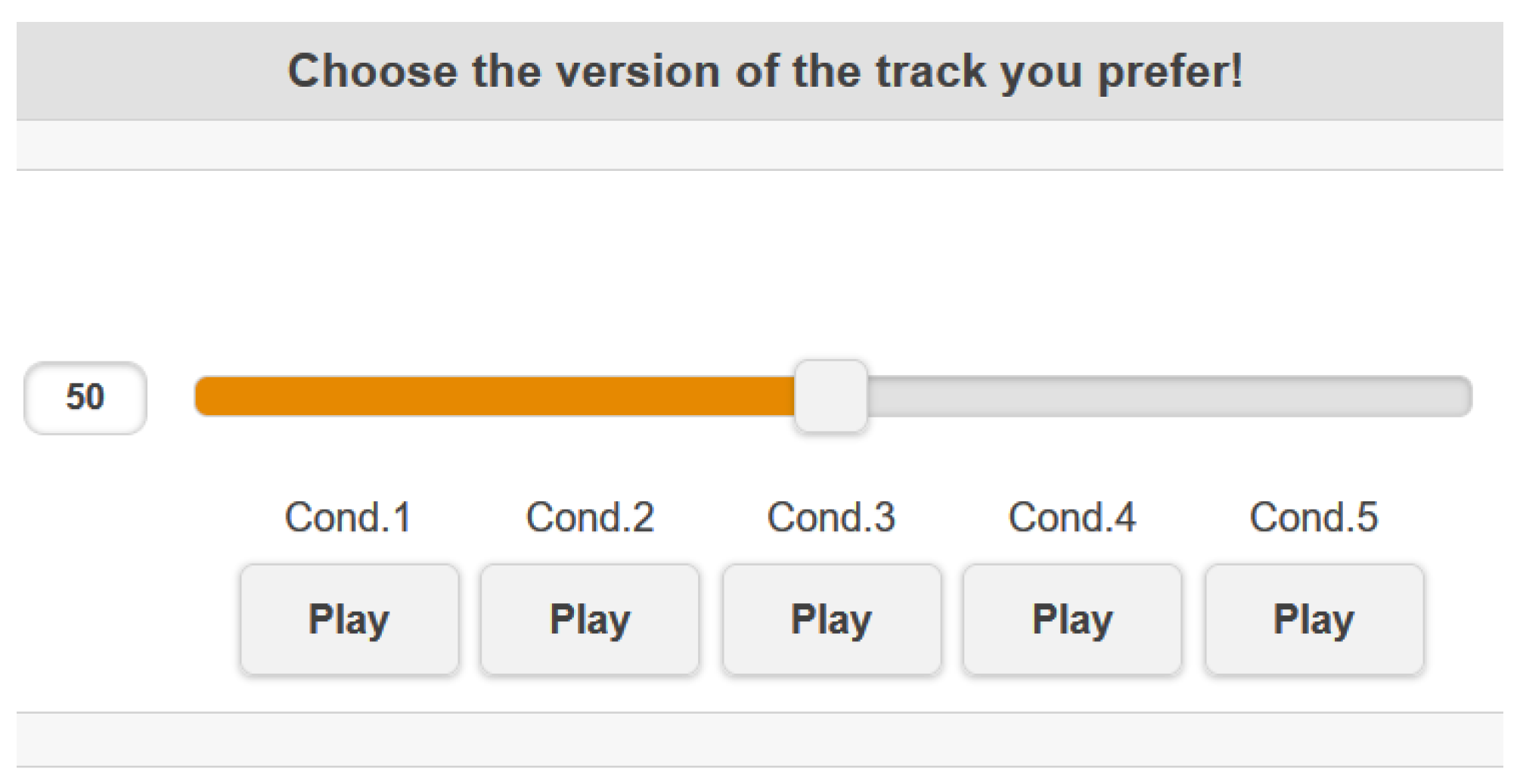
Figure 6.
Graphical user interface of the experimental procedure. Cond.1–Cond.5 correspond to the differently processed versions of the same song. The slider bar corresponds to the volume.
Figure 6.
Graphical user interface of the experimental procedure. Cond.1–Cond.5 correspond to the differently processed versions of the same song. The slider bar corresponds to the volume.

Figure 7.
Equalization preference for highly (N = 22) and lowly (N = 23) aroused listeners, for all tracks.
Figure 7.
Equalization preference for highly (N = 22) and lowly (N = 23) aroused listeners, for all tracks.

Figure 8.
Equalization preference (a) for highly (N = 22) and (b) and lowly (N = 23) aroused listeners, for the different genres.
Figure 8.
Equalization preference (a) for highly (N = 22) and (b) and lowly (N = 23) aroused listeners, for the different genres.

Figure 9.
Equalization preference (a) for highly (N = 22) and (b) lowly (N = 23) aroused, for every single track.
Figure 9.
Equalization preference (a) for highly (N = 22) and (b) lowly (N = 23) aroused, for every single track.

Figure 10.
Equalization preference for highly (N = 37) and lowly (N = 9) pleasured listeners, for all tracks.
Figure 10.
Equalization preference for highly (N = 37) and lowly (N = 9) pleasured listeners, for all tracks.

Figure 11.
Equalization preference (a) for highly (N = 37) and (b) and lowly (N = 9) pleasured listeners, for the different genres.
Figure 11.
Equalization preference (a) for highly (N = 37) and (b) and lowly (N = 9) pleasured listeners, for the different genres.

Figure 12.
Equalization preference (a) for highly (N = 37) and (b) for lowly (N = 9) pleasured listeners, for every single track.
Figure 12.
Equalization preference (a) for highly (N = 37) and (b) for lowly (N = 9) pleasured listeners, for every single track.


Table 1.
Equalization settings of the 5 predefined equalization curves used in the experiment. and G denote the cut-off frequency and the gain for shelving filters, respectively. , , and denote the central frequency, the gain, and the quality factor for parametric EQs (peaking filters), respectively, with .
| Equalization | Filter Type | Settings | ||
|---|---|---|---|---|
| Low Shelving Filter | Shelving | kHz | dB | |
| High Shelving Filter | Shelving | Hz | dB | |
| Midrange Boost Filter | 3 Parametric EQs | kHz | dB | |
| kHz | dB | |||
| kHz | dB | |||
| Midrange Dip Filter | 3 Parametric EQs | kHz | dB | |
| kHz | dB | |||
| kHz | dB | |||
| Transparent (No Filter) | − | − | − | − |
Table 2.
Tracks dataset used in the experiment. “Label” column refers to the label of track, as used in the present paper; “Track name” refers to the actual title of the track and the artist, as found in the online repository.
Table 2.
Tracks dataset used in the experiment. “Label” column refers to the label of track, as used in the present paper; “Track name” refers to the actual title of the track and the artist, as found in the online repository.
| Label | Track Name |
|---|---|
| Classic 1 | Brandenburg Concerto No. 3 in G major, BWV 1048, Bach |
| Classic 2 | La Vie (interlude), Manumusic |
| Jazz 1 | One, Paolo Pavan Quartet |
| Jazz 2 | Old Fashioned Love Song, Prart |
| Rock 1 | Rosa, Deputies |
| Rock 2 | The Symphonic Muse, Peter Swart |
| Pop 1 | Everything I’m Not, FromTom |
| Pop 2 | Breathing in, Turxmuzic |
| Soul 1 | Outta My Head, BruceJames |
| Soul 2 | From my window, Sharpword |
Table 3.
Mapping of the 15 categorical mood descriptors to arousal and pleasure binary categorization (“High” and “Low”).
Table 3.
Mapping of the 15 categorical mood descriptors to arousal and pleasure binary categorization (“High” and “Low”).
| Mood Descriptor | Arousal | Pleasure |
|---|---|---|
| Alert | High | High |
| Excited | High | High |
| Elated | High | High |
| Happy | High | High |
| Contented | Low | High |
| Serene | Low | High |
| Relaxed | Low | High |
| Calm | Low | High |
| Bored | Low | Low |
| Depressed | Low | Low |
| Sad | Low | Low |
| Upset | High | Low |
| Stressed | High | Low |
| Nervous | High | Low |
| Tense | High | Low |
Table 4.
The “Majority” rule used for mapping multiple arousal and pleasure binary categorization values (i.e., High and Low) as resulted from the mood descriptors, to single arousal and pleasure binary categorization values (i.e., High and Low). All mood descriptors (i.e., Mood Descriptor 1, Mood Descriptor 2, and Mood Descriptor 3) have the same “dominance” over listeners’ mood, irrespective of the presentation order. Thus, all possible combinations are presented in this table.
| Mood Descriptor 1 | Mood Descriptor 2 | Mood Descriptor 3 | Final Mood |
|---|---|---|---|
| High | - | - | High |
| Low | - | - | Low |
| High | High | - | High |
| Low | Low | - | Low |
| High | Low | - | Excluded |
| High | High | High | High |
| Low | Low | Low | Low |
| High | High | Low | High |
| High | Low | Low | Low |
Table 5.
Number of participants over the different arousal and pleasure states.
| Arousal | Pleasure | |
|---|---|---|
| High | 22 | 37 |
| Low | 23 | 9 |
| Total | 45 | 46 |
Table 6.
Values of p for each track, exploiting the Fisher’s exact test for the arousal analysis.
| Track | p Value | Track | p Value |
|---|---|---|---|
| Classic 1 | 0.816 | Rock 1 | 0.028 |
| Classic 2 | 0.402 | Rock 2 | 0.113 |
| Jazz 1 | 0.047 | Soul 1 | 0.539 |
| Jazz 2 | 0.281 | Soul 2 | 0.082 |
| Pop 1 | 0.130 | ||
| Pop 2 | 0.846 |
Table 7.
Values of p for each track, exploiting the Fisher’s exact test for the pleasure analysis.
| Track | p Value | Track | p Value |
|---|---|---|---|
| Classic 1 | 0.623 | Rock 1 | 0.242 |
| Classic 2 | 0.076 | Rock 2 | 0.161 |
| Jazz 1 | 1.000 | Soul 1 | 1.000 |
| Jazz 2 | 1.000 | Soul 2 | 0.466 |
| Pop 1 | 1.000 | ||
| Pop 2 | 0.824 |
Publisher’s Note: MDPI stays neutral with regard to jurisdictional claims in published maps and institutional affiliations. |
© 2022 by the authors. Licensee MDPI, Basel, Switzerland. This article is an open access article distributed under the terms and conditions of the Creative Commons Attribution (CC BY) license (https://creativecommons.org/licenses/by/4.0/).
Share and Cite
MDPI and ACS Style
Dourou, N.; Bruschi, V.; Spinsante, S.; Cecchi, S. The Influence of Listeners’ Mood on Equalization-Based Listening Experience. Acoustics 2022, 4, 746-763. https://doi.org/10.3390/acoustics4030045
AMA Style
Dourou N, Bruschi V, Spinsante S, Cecchi S. The Influence of Listeners’ Mood on Equalization-Based Listening Experience. Acoustics. 2022; 4(3):746-763. https://doi.org/10.3390/acoustics4030045
Chicago/Turabian StyleDourou, Nefeli, Valeria Bruschi, Susanna Spinsante, and Stefania Cecchi. 2022. "The Influence of Listeners’ Mood on Equalization-Based Listening Experience" Acoustics 4, no. 3: 746-763. https://doi.org/10.3390/acoustics4030045