
Locating Sources of Vibration with Harmonics and Pulse Signals in Industrial Machines


Department of Oil and Gas Transportation and Storage, Ufa State Petroleum Technological University, 450064 Ufa, Russia
*
Author to whom correspondence should be addressed.
Acoustics 2022, 4(3), 574-587; https://doi.org/10.3390/acoustics4030036
Submission received: 13 June 2022
/
Revised: 24 July 2022
/
Accepted: 27 July 2022
/
Published: 29 July 2022
Abstract
:This paper is devoted to a new approach to condition monitoring. The main feature is an application of strain gauge analysis for geometrical locating of vibrating defects. Information about the exact geometrical location of a defect, intensity of excitation and its frequency provides accurate diagnostics. The research contains theoretical and experimental parts. Three types of defects are analyzed: defects with harmonic parameters, defects with non-harmonic periodical parameters (pulse periodic signal) and defects with non-periodical parameters (pulse non-periodical signal). For the first type, analysis of micro movements in the equipment is used. The others use triangulation; for detecting time lag of signal approaching in each sensor, an analysis of phase spectrum is used. This method can find sources of vibration/defects with pulse-like signals. An electronic board and computer program for implementation of the proposed method are developed. The electronics measure strain gauge data in real time and transmit it to a computer program. Such an approach gives new information for diagnostics and provides new opportunities for effective defect detection and condition monitoring of various machines and equipment.
1. Introduction
When operating responsible industrial machines, there is always the task of ensuring the reliability of their operation, including such indicators as durability and operability. The factors that reduce reliability are failures; hence, it is important to minimize the probability of their occurrence.
The tools for reducing the probability of failures (i.e., increasing the reliability of the equipment) are methods of technical diagnostics, including methods for determining incipient defects. Timely elimination of defects makes it possible to eliminate accidents and ensure uninterrupted operation of the equipment in a given period of time.
In this paper, only methods for determining defects, which can be automated and implemented during equipment exploitation, are discussed. Today, various methods of technical diagnostics are used for industrial equipment:
- operation parameters diagnostics (such as flow rate, energy consumption, efficiency, pressure, etc.) [1];
- overall vibration level control [2];
- spectral diagnostics (analysis of vibration signal) [3];
- infrared thermography [10];
- ultrasound propagation analysis [11];
- acoustic noise signal analysis [12];
- wavelet analysis [13];
- 3D vibration spectra analysis [14];
- location of oscillation defects by remote strain gauge analysis [17];
- and some others.
The most interesting methods of technical diagnostics are those that can be easily automated, deal with large numbers of possible defects and provide operative results. Good possibilities can be provided by means of various methods of vibration analysis. However, for example, analysis of the vibration spectrum also has some problems: vibration sensors measure vibration levels not at the source of vibrations, but at some distance from it. In fact, the vibration sensor measures the vibration level of a point that differs from the point being analyzed. Moreover, during the transmission of the signal from the vibration source to the sensor, its distortion occurs; additional modulation due to noise, resonances and distortions appears. Vibration diagnostics has a significant noise level, i.e., during normal operation of the equipment, the vibration level can fluctuate between 2–5 mm/s (e.g., for oil pumping units), while the normal noise level is 0.3 mm/s, which is more than 10%.
Control of electric motor parameters and so-called sensorless control [18,19] gives an opportunity to analyze technical condition not just of an electric drive, but also of machines in general. Obviously, however, this method does not allow diagnosing all defects of the whole unit.
Continuous operation leads to the fact that within the framework of diagnostics, it is impossible to carry out any manipulations directly in the defect zone. It follows from this that all methods for localization, identification of defects, as well as determining their danger, are indirect.
For equipment that has been in operation for many years, an experimental base of developments is used; features of all kinds of defects can be fixed. In that case, it is traditional to install sensors (usually vibration sensors) in the most critical places. Further, according to the data obtained and the available database of defects, the defect is empirically determined.
For new equipment that does not have significant experience, this approach does not work. That is the reason why intelligent condition monitoring of machines using machine learning cannot be freely applied at this moment, although there are many good researches in this field that have appeared in the last few years [20,21,22,23]. Additionally, this approach is poorly feasible for complex equipment, including those with multiple shafts, such as gas pumping units. In this case, the features of defects may overlap with each other. So, it is hard to analyze them.
Therefore, for reliable diagnostics of both new and complex pumping equipment, it is necessary to develop and use new diagnostic approaches that ensure the principle of information redundancy.
Thus, the purpose of this study is to develop methods for localization of defects (i.e., sources of vibration) in space. These methods should have an ability to be automated and work in real-time. The study of the methods is devoted to rotary machines, such as pumps, compressors, engines, fans, etc. Thus, additional and relevant information for the diagnosis of defects may be information about the location of the defect, or in the general case of the source of excitation, in space. Information about which part of the equipment, in which node, the source of excitation is located will fundamentally narrow the list of possible defects. So, if there is a drawing of the equipment and a specification of all the nodes containing information about their location and masses, it is possible to accurately identify the defective part of the equipment. This approach is relevant for new equipment for which a large experimental base for its operation has not yet been developed and a detailed defective map has not been prepared.
This study is devoted to geometrical localization via remote strain gauge sensors of various types of defects creating excitation force with harmonic parameters, non-harmonic parameters (pulse periodic signal) and non-periodical parameters (pulse non-periodical signal).
2. Concept of the Method of Locating Defects with Periodical and Non-Periodical Parameters Using Strain Gauge Signal Analysis at Specified Points
In general, defects and various vibration sources can be classified into three big groups:
- defects with harmonic parameters;
- defects with non-harmonic periodical parameters (pulse periodic signal);
- defects with non-periodical parameters (pulse non-periodical signal).
As for the three groups of defects mentioned, the first one presents various sources of vibration that create constant periodic oscillations in the equipment. An example of such defects is an imbalance. Signal analysis (strain gauges signal analysis or vibration signal analysis—it works for both) in this case shows an almost perfect sine wave in time, and when the signal is decomposed into a spectrum, a single pronounced peak.
Non-harmonic periodic vibration sources are those defects that have a periodic nature, but are not described by a single sinusoid. An example of such defects may be bearing defects. In this case, strain gauge sensors show a complex periodic signal in time; and when decomposed into a spectrum, several peaks. Non-periodic vibration sources are those that do not relate to the cases mentioned above. In particular, the signal spectrum in this case is characterized by a non-constant set of harmonics with a large amount of noise.
The third type, i.e., defects with non-periodical parameters, is the most difficult for analyze. It can be defects of a hydrodynamic nature, random shocks, touching of the shoulder blades, etc.
So, the approach to these types of defects should be different.
In this study, methods for identifying and locating all three groups are proposed. Methods use the same equipment for diagnostics: strain gauge sensors and special electronics. According to the proposed idea, in order to detect the defects, it is necessary to install load cells either on supports or under them. This approach has a very important advantage: the sensors use the resistive method to measure strain, i.e., force in this case. Hence, applying an analog signal amplifier and primary signal processing allow obtaining a very high rate of signal measurement. Authors have registered the signal delay of a few microseconds.
Moreover, strain gauge sensors have almost no limitations on the frequency of signal measurement. It allows obtaining higher sensitivity and more possibilities for analysis.
Sources of excitation or defects create dynamic forces in the equipment, which are measured by the load cells in real time. With the help of an algorithm, which is presented below, it is possible to determine the coordinates of the defects and build a three-dimensional graph of their location.
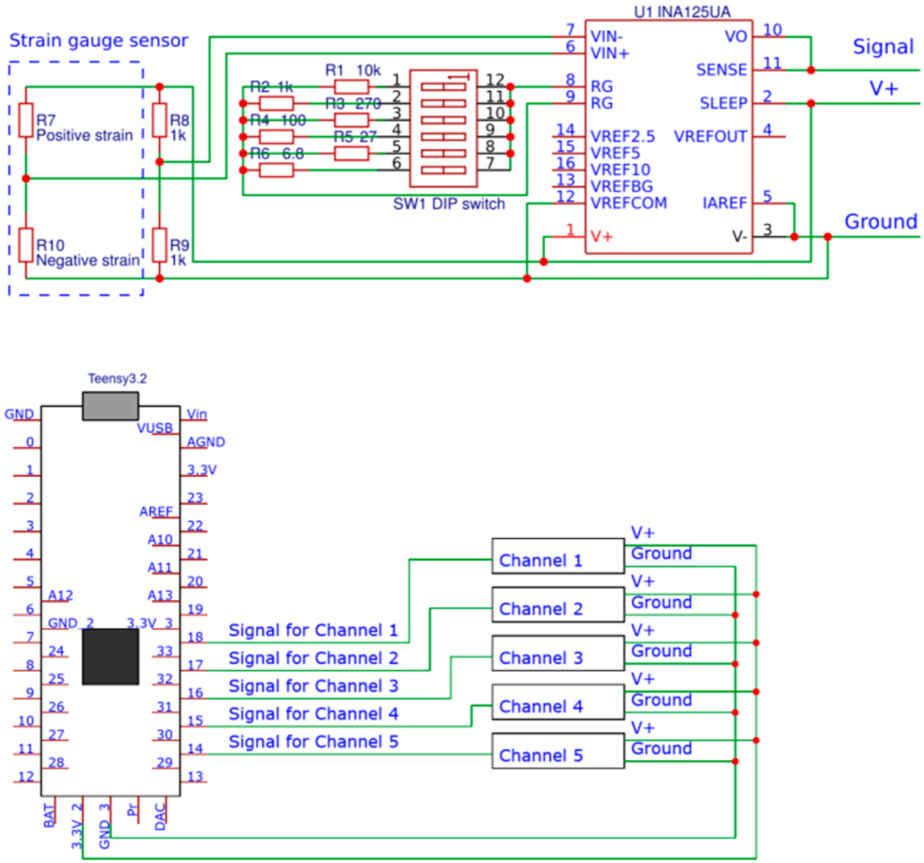
For implementing the methods, the following experimental electronic rig is used. It contains four strain gauge sensors located under machine supports. It also contains a printed circuit board (Figure 1) with INA 125 amplifiers with various amplifying coefficients and a Teensy 3.2 microcontroller with integrated 12-bit analog-to-digital converter for data collection. The data are transferred to a computer via a USB port and a serial communication protocol. A microcontroller sends consequential requests from strain gauge sensors every 9 microseconds. Analysis in a computer is performed via an experimental program written in the Python language.
The experimental rig (Figure 2) includes a base with dimensions of 90 cm × 30 cm × 4 cm, weighing 5.6 kg, on which 5 fans with an eccentric are located, representing excitation sources. Fans are slightly changed in order to have eccentricity and simulate blade touching. Each fan is equipped with a PWM speed controller, which allows one to smoothly change the speed of rotation of the shaft.
3. Locating Defects with Harmonic Parameters Using Strain Gauge Signal Analysis at Specified Points
Locating defects with harmonic parameters using strain gauge signal analysis at specified points uses the principle of detecting micro movements in equipment. Vibration sources cause longitudinal and rotational micro movements in it. The horizontal vibration projections cause micro “swinging” in the equipment, hence the dynamic reactions on the equipment supports are different in phase. So, measuring the amplitudes and phases of the dynamic reactions on the supports can help to locate the vibration source. This information can serve to accurately and reliably identify a defect.
The amplitudes and phases of the dynamic reaction on the supports can be measured by application of load cells under supports or on the equipment frame. With electronics and high rate signal measuring, one can obtain the spectrum of dynamic reaction on each support; hence calculating the amplitudes and phases.
This provides the relationship between the defect location, the amplitudes and the phases of dynamic reactions. The corresponding analysis and derivation of formulas are omitted in this paper. The derivation can be taken from the authors’ previous study [17]. Only final formulas used to calculate the exciting force coordinates are presented.
The horizontal coordinate of the exciting force or a defect point of application (distance from the support A) equals to:
where φA is the oscillation phase of the reaction of the support A; φB is the phase of the oscillations of the support reaction B; φF—phase of oscillation of the sum of reactions in the supports A and B; RA—the response amplitude in the support A; RB—the reaction amplitude in the support B; x and z—horizontal coordinate; y—vertical coordinate.
Similarly, we calculate the position of the excitation source or a defect along the z axis (the horizontal axis perpendicular to the x axis):
The height of the excitation source or a defect, i.e., y-coordinate, equals:
Thus, the formulas for calculating the 3D position of a defect are received.
To locate a defect, it is necessary to consistently apply Formulas (1)–(3). The first two formulas should be applied in two vertical planes, which are parallel and perpendicular to the rotor axis. Formula (3) gives the vertical coordinate of a defect.
Note that these formulas can be applied only for the defects with harmonic parameters, i.e., the intensity of oscillations made by a defect is constant, and its frequency does not change in time. Additionally, the accuracy of these formulas is better for the defects with oscillations provided by harmonic law, such as rotor eccentricity.
4. Locating Defects with Non-Harmonic Periodical Parameters Using Strain Gauge Signal Analysis at Specified Points
Locating defects with non-harmonic periodical parameters is based on the following idea.
It is considered that a pulse from the defect moves to the sensors almost in a straight line with the speed of propagation of acoustic waves in the metal of the equipment housing. Accordingly, the later the pulse reaches a certain sensor, the further away the defect is from it; then, using triangulation methods, it is possible to determine its location in space. Obviously, it is most convenient to place the sensors at a distance from each other, that is, in the corners of the equipment.
However, conditioned on the dimensions of the equipment, pulses reach sensors at almost the same time, and there is a technical problem of determining the difference in the time of their passage. For single pulses, this remains a problem, but it can be solved under the condition of information redundancy for a large number of pulses based on the fact that the pulses are periodic.
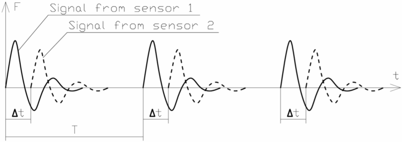
Consider a signal that reaches two sensors in a conditional example. Let the pulse reach one sensor later by the time Δt relative to the other (Figure 3). Consider that Δt is many times smaller than the pulse repetition period T: Δt << T. In this case, the signal from sensor 2 repeats the signal from sensor 1 in shape, but possibly with a different vertical scale.
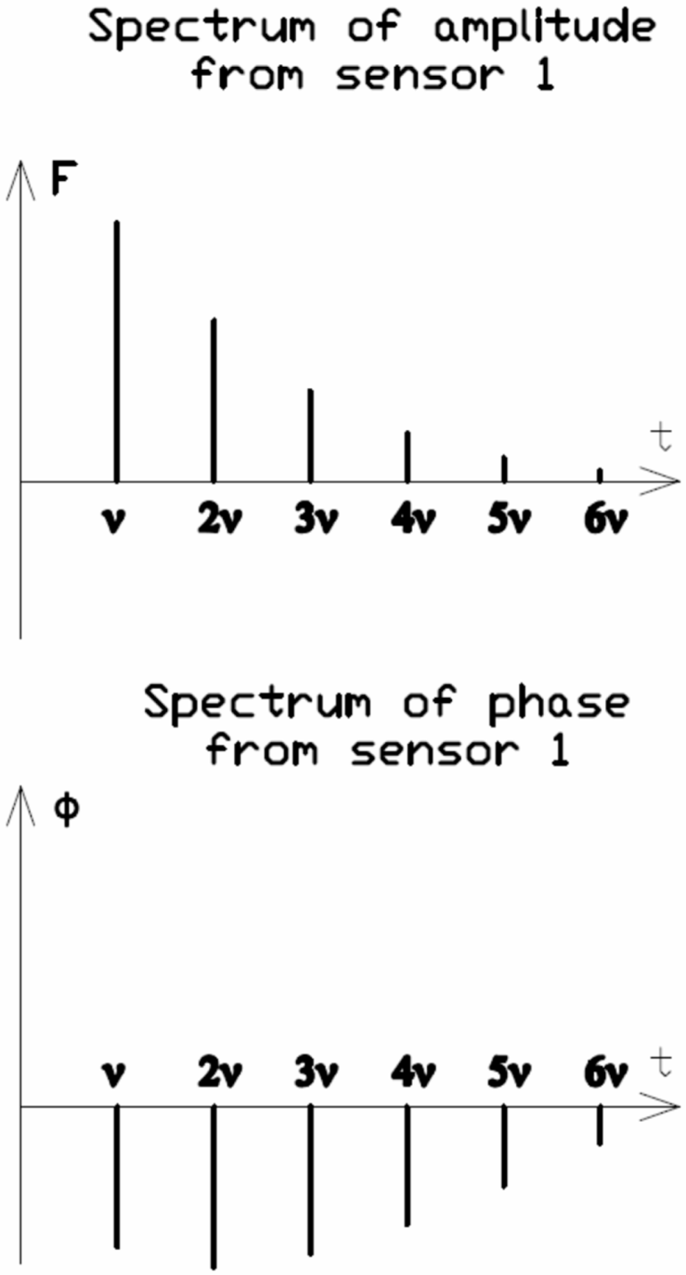
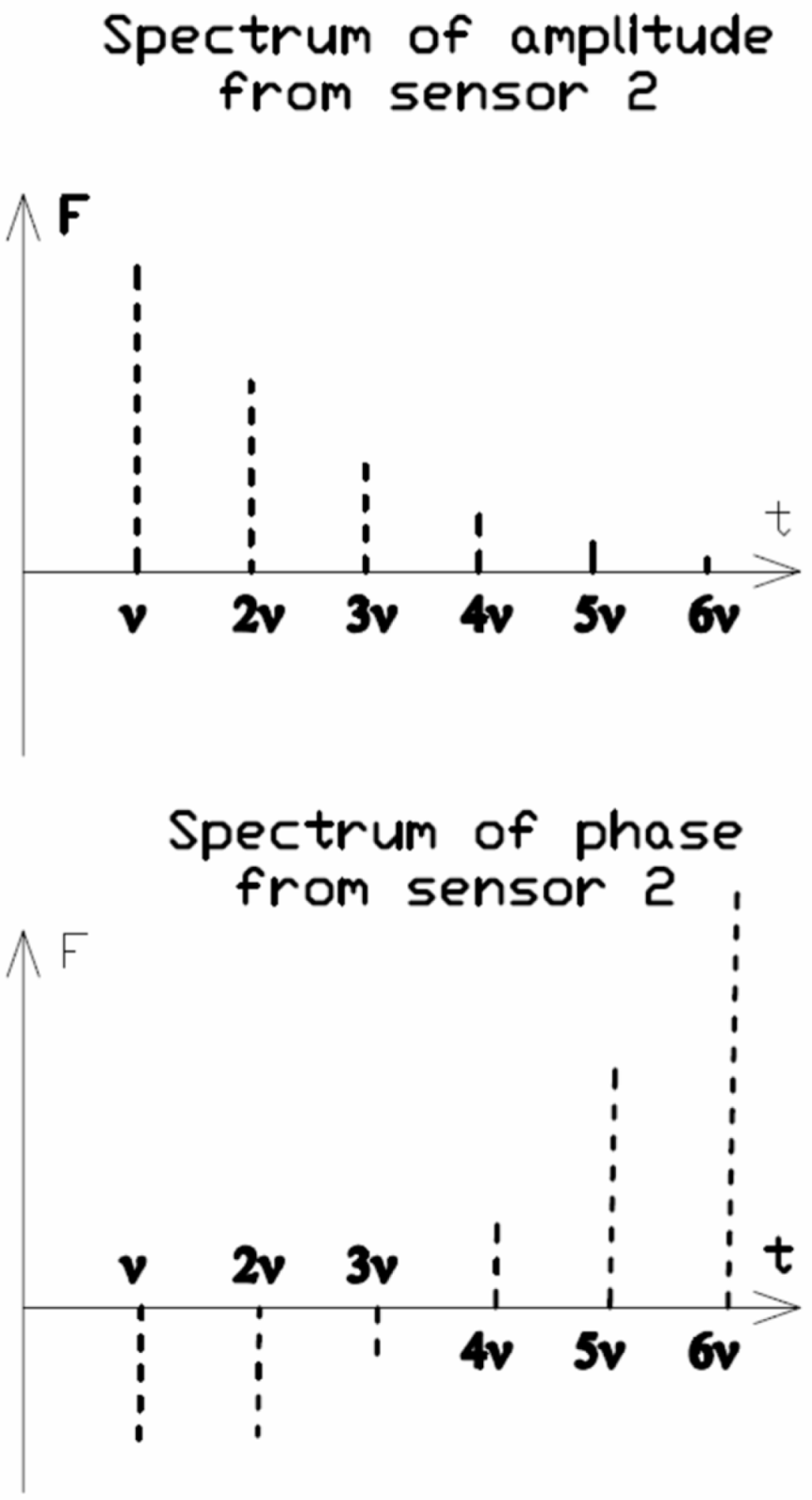
Next the signal from the sensors into a spectrum of amplitudes and a spectrum of phases is decomposed (Figure 4 and Figure 5).
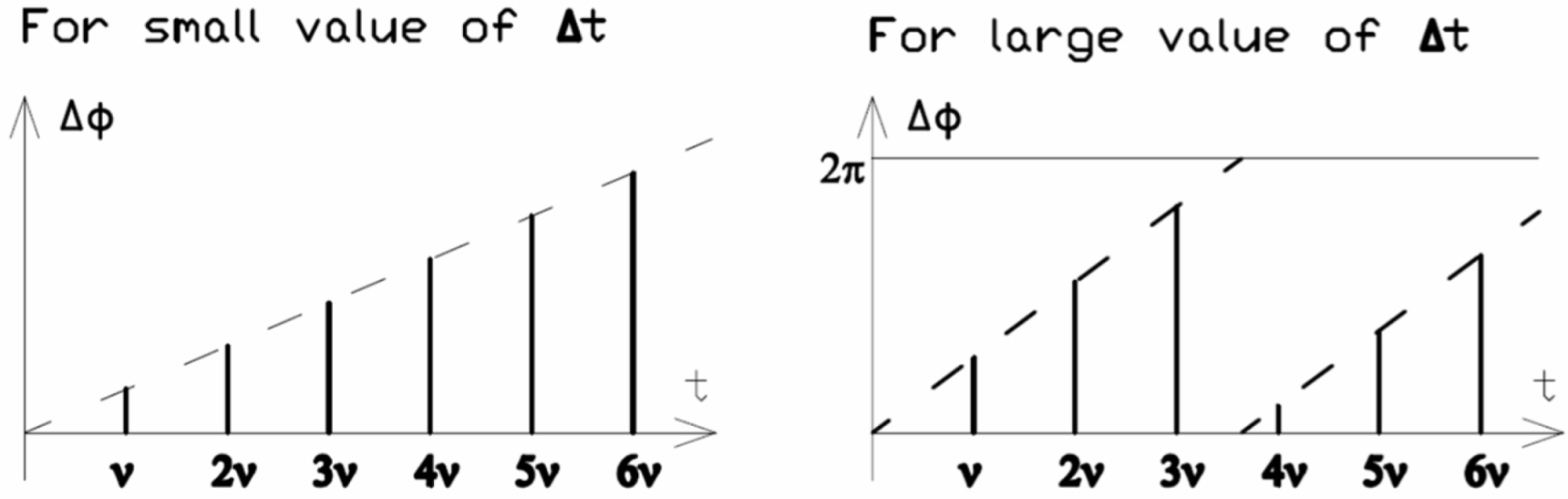
Since the pulse source is single, the signal reached by both sensors has the same shape, and the signal in amplitude spectra for both sensors is similar. At the same time, since the signal is not harmonic, a set of peaks at frequencies that are multiples of the frequency of occurrence of the signal v = 1/T is always visible on the amplitude spectrum. However, the phase spectra are different, and the more one signal lags behind the other, the more they differ. Thus, this circumstance can be used to determine the value of Δt.
Next a graph that shows the difference in the values of the two phase spectra is built (Figure 6).
On a graph with a difference in phase spectra from two sensors, all points are shifted by the same value (by analogy with the phase spectra of the shifted function of rectangular pulses). Accordingly, they lie on one straight line coming out of zero, or in the case of a large value of Δt, they are located on a group of parallel lines (Figure 6).
This fact can be explained as follows. The signal from sensor 2 f2(t) lags behind the signal from sensor 1 f1(t) by the value Δt. Given that the amplitude of the signal between them may differ by k times, then using the discrete Fourier transform, the following dependencies can be written for them:
where ai and βi are the harmonic phases for the i-th component in the Fourier decomposition; Ai is the harmonic amplitude for the i-th component in the Fourier decomposition; v1 is the pulse frequency; t is the time; n is the number of harmonics in the Fourier decomposition.
For two functions to be equal, the components associated with cosines must be equal; therefore, the arguments for cosines must be equal or differ by a multiple of 2π:
Thus, the phase difference for frequency vi expressed as Δφi = βi − ai equals to:
Thus, Δφi, as a function of the frequency i·v1, is either a straight line passing through the origin, or a set of straight lines, as shown earlier (Figure 5).
The angle of inclination of the line on the graph of the phase spectrum difference (Figure 5) is directly related to the magnitude of the lag of the signal Δt, so for its definition, it is necessary to construct this line, which, in fact, is approximating for the set of points obtained. Using the least squares method, the following condition (we assume that the line passes through the origin) is obtained:
where φi are the values of the phase difference on the spectra of the two signals (Figure 5) after measurements and transformations.
It should be noted that in practice, it is extremely likely that there is some other defect at the v1 frequency, for example, the eccentricity of the rotor, so it is recommended to exclude this frequency from the analysis, so we build a line from a point at the frequency 2·v1:
The solution of this equation allows determining the desired value of Δt.
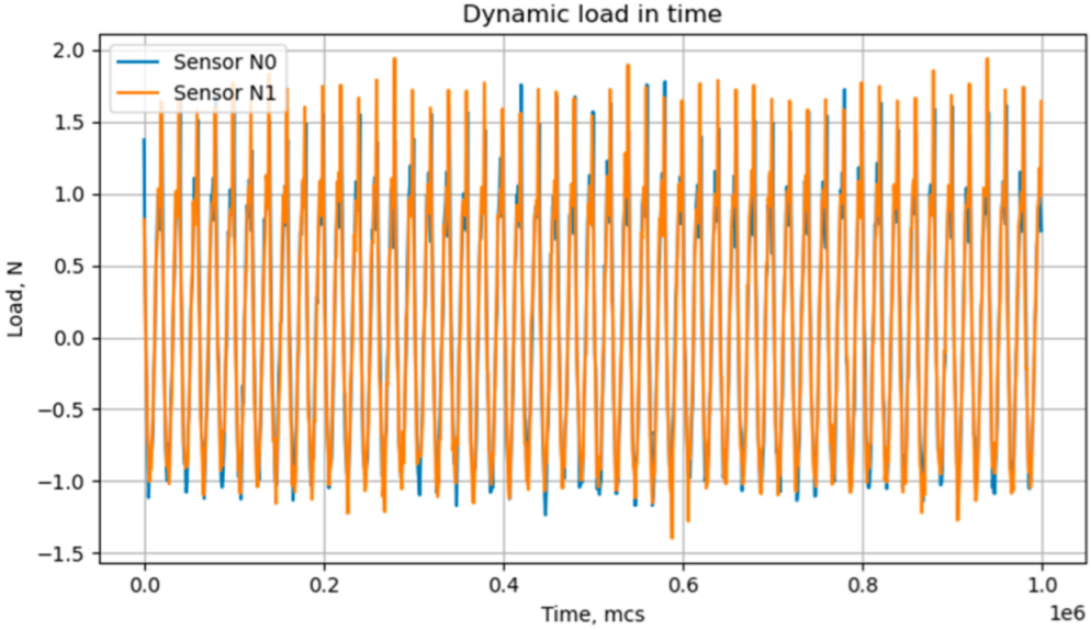
Let us test this method on a conditional example. It is considered that on some pump, there is a touch of the body blade. Accordingly, there are fluctuations due to the imbalance of the rotor, as well as a repetitive shock pulse. It is considered that the point of contact with the body blade is at a distance from the sensors with such a difference that the pulse reaches with a delay of Δt = 1 ms (the value is taken for clarity of the image of the subsequent graphs; in real conditions this value will be less). It is assumed that the imbalance creates a harmonic with amplitude of 1 N and a frequency of 50 Hz on the load cells, and the shock pulses have a peak of 0.5 N. It is also assumed that there is noise in the sensors, which we simulate with a random signal with a normal distribution with a standard deviation of 0.1 N. That means that the signal-to-noise ratio equals 100. Additionally, it is assumed that the signal measurement occurs simultaneously from both sensors with an interval of 1 ms (1000 Hz), and the number of measurements is 1000.
The graph of the simulated signal shows that there is a signal with a certain noise (Figure 7).
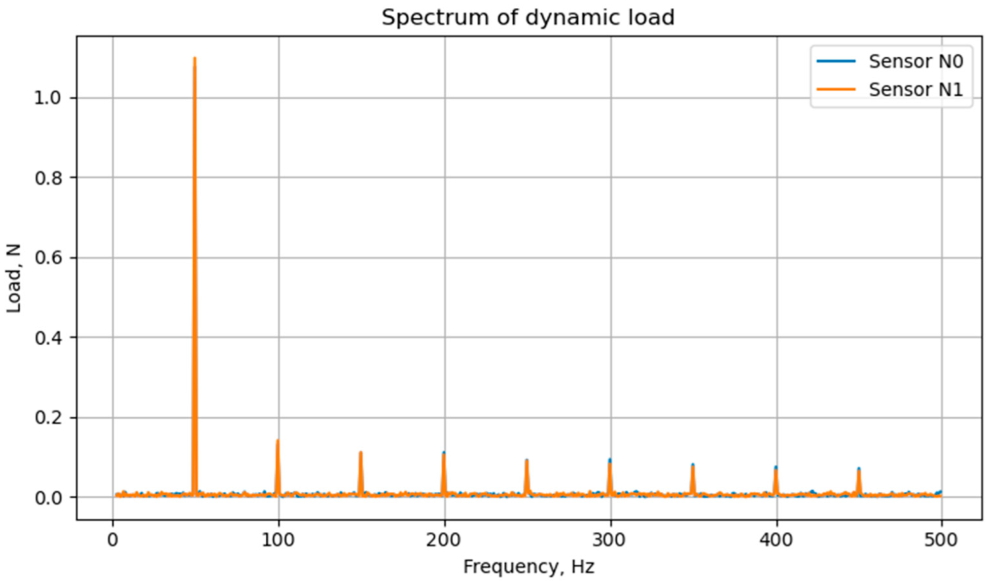
The decomposition of the signal into a spectrum obviously shows a peak at a frequency of 50 Hz, reflecting the imbalance of the rotor, as well as a set of decreasing harmonics and a certain noise level (Figure 8).
The phase spectrum constructed with a filter for amplitudes less than 0.001 N (Figure 9) shows a seemingly chaotic picture. This is due to the fact that for noise when the signal is decomposed into a Fourier series, despite the relatively small amplitude, the phase can have a value in the interval (−π; π). Additionally, taking into account the randomness of the noise, then the resulting phase will also have a random value in this range and in general occupy a solid area on the graph.
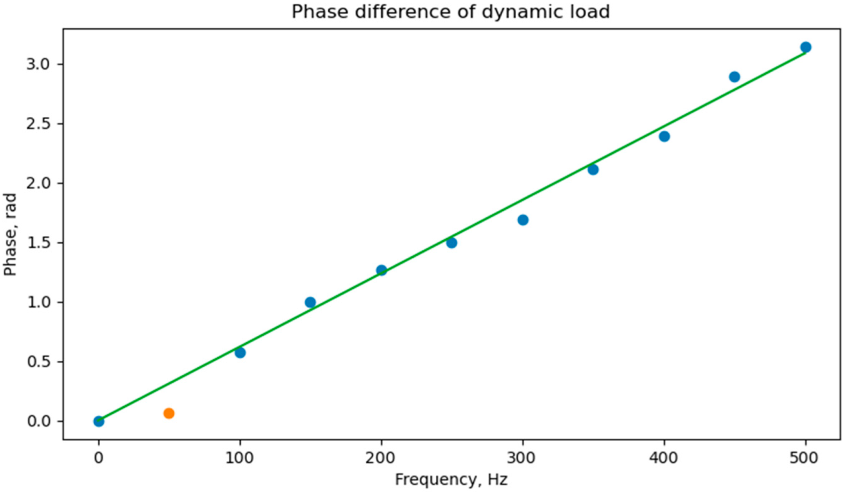
However, if all bands with noise are removed from the resulting phase spectrum, in other words, only bands at frequency multiples of 50 Hz are left, then a pattern will already be observed. If we plot the phase difference of the signals for two sensors, we obtain a line graph (Figure 10). Some deviation of points from a straight line is caused by the presence of noise. We note that the point at a frequency of 50 Hz is significantly out of linear dependence, since there is another defect at this frequency; hence, this point is not taken into account in the subsequent analysis.
The value of the time delay Δt can be determined by solving Equation (6), or defined as the angle of the slope of a straight line to the abscissa axis divided by 2π, taking into account the dimensions of the graph. The solution of the equation leads to the value Δt = 1.013 ms. Thus, in a conditional example, the method shows very high accuracy.
5. Locating Defects with Non-Periodical Parameters Using Strain Gauge Signal Analysis at Specified Points
Defects with non-periodical parameters could not be located by such spectrum analysis, because the spectrum analysis requires a stable harmonic signal to obtain proper data. Such defects can be located only with high rate measurements. Modern electronic measuring tools provide data with a rate of around 1 MHz, and modern computer possibilities allow processing this data in real time. This allows analyzing each impulse produced by the excitation source. Such data gathering rates yield an approximate coordinate assessment error of a few centimeters.
Shock waves propagate through the equipment material at the speed of sound. High rate analysis of signal in signal allows showing the position of a shock source with the help of the following system of equations:
Here ta, tb, tc, td are pulse propagation times to each of the sensors, t0 is pulse movement start time; Lx, Ly and Lz are equipment dimensions; v is speed of wave propagation in material of equipment; x, y, z are the excitation source coordinates that should be obtained.
It is assumed that the speed of wave propagation is already known. When it is unknown, it can be easily calculated by a test with a known defect by artificial knocking on the equipment surface at certain points.
To implement the diagnostics in real time, this system of equations has to be solved very quickly. However, the problem is that this system cannot be solved explicitly. So, there can be various methods of solution.
The first way is to transform the system of equations into a single target function that has to be minimized like the following:
Minimizing can be achieved numerically. Limits for the variable are as follows:
Minimizing should be conducted with a fast algorithm. An example of such an algorithm is the Nelder–Mead method or a similar one.
The second method is to apply a set of preliminary solutions for the system of Formula (4). It means that first, the system should be solved for various combinations of parameters and that a predictive model should be created. Such a model can be created via machine learning as a regression model basing on algorithms such as “Decision tree” or “Nearest neighbors”.
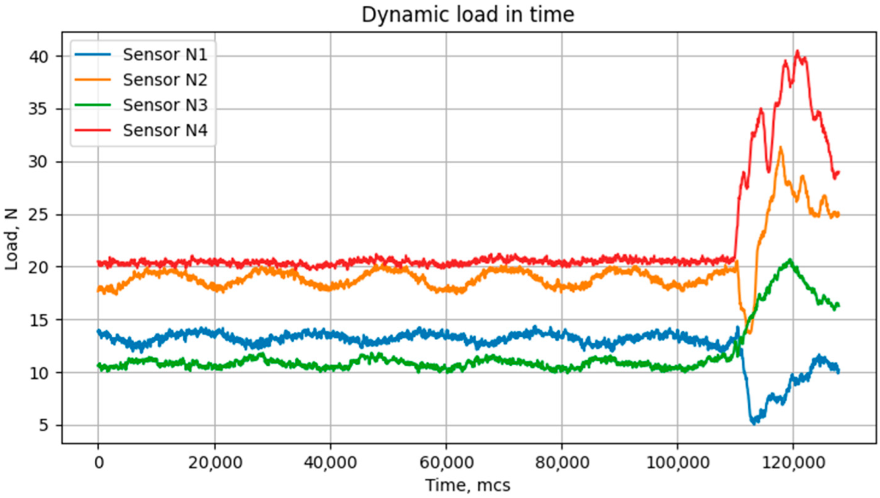
An example of a pulse signal received by this electronic rig is shown in Figure 11.
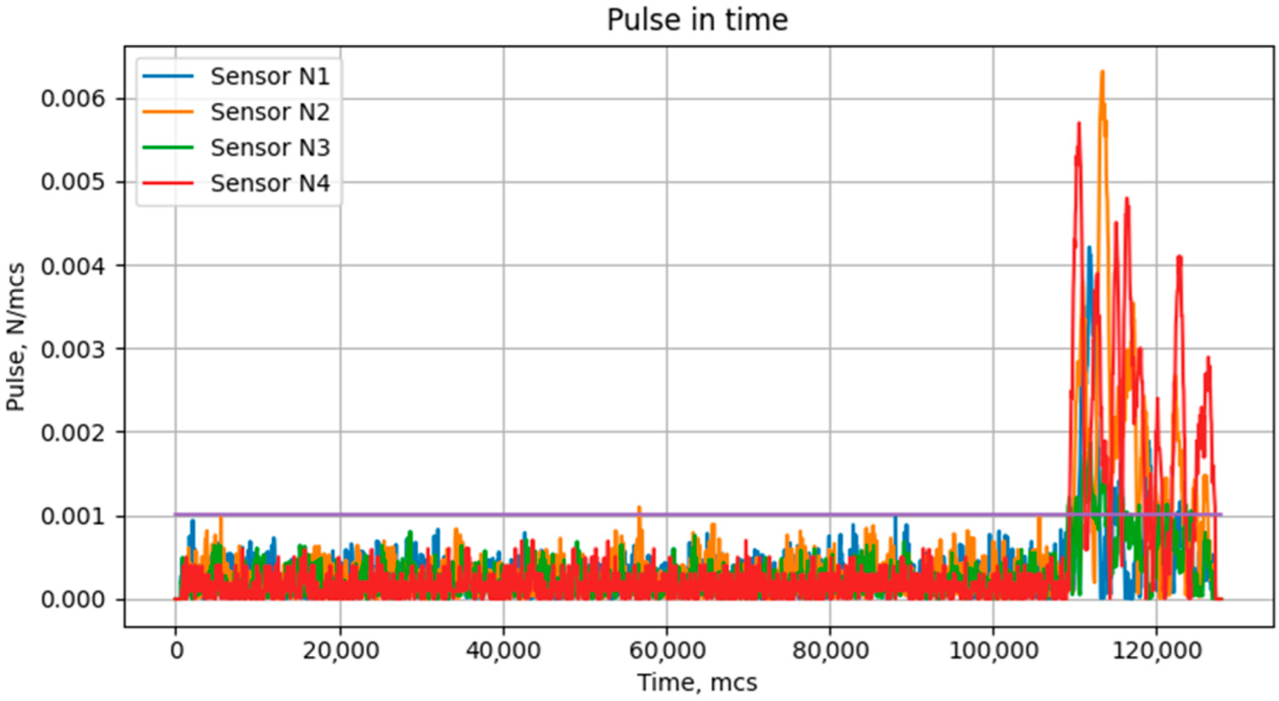
A random pulse hitting the surface of the laboratory pump is clearly seen in Figure 4. However, we need a method to distinguish a random sharp pulse from a vibration with a stable harmonic signal. For this, we can use the value of the derivative of the signal. As shown in Figure 12, the random pulse is more distinct than that in Figure 11.
To automatically detect a sharp increase in the signal value derivative, the following criteria are suggested:
Here, Rcritical is a critical value of the signal value derivative, Raverage is an average value of this variable, σ is its standard deviation. From the theory of probability, it follows that if k = 2, the noise is filtered with 95% probability.
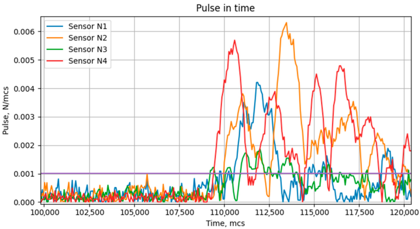
A detailed graph of the signal value derivative increase for each of four strain gauge sensors is shown in Figure 13.
The signal lines intercept the critical value of a signal value derivative of different points. This means that the pulse reaches sensors 1, 2, 3, and 4 at various moments. The application of Formula (11) allows calculating the location of a random pulse source made by the defect.
6. Conclusions
The proposed diagnostic method using strain gauge data allows determining the coordinates of the defect. When processing the signal, the excitation frequency and the excitation intensity of a defect can be calculated.
The method allows detecting defects of industrial equipment with periodical and non-periodical parameters. The defects of the first type are detected based on the fact that the excitation sources produce micro movements that can be classified as longitudinal and rotational. Hence, the dynamic reactions on equipment supports are not simultaneous, i.e., have different phase. The analysis of these reactions can give the values for the intensity and frequency of a defect, and also allows calculating the coordinates.
The defects with periodical and non-periodical parameters are proposed to be detected via pulse control of a high frequency signal analysis.
Accordingly, three types of additional information for the equipment diagnostics become available. So, the location gives the principal location of a defective node. Furthermore, if various potentially defective parts are found at a certain point at once, then a differentiation can be made based on the information about the frequency and intensity of vibrations.
So, if there is a drawing of the equipment and a specification of all the nodes containing information about their location and masses, it is possible to accurately identify the defective part of the equipment.
With the experimental rig, the principal possibility of using the proposed method for localization of defects was shown.
This approach is relevant for new equipment for which a large experimental base for its operation has not yet been developed and a detailed defect map has not been prepared. Further, the method may increase the reliability of diagnostics for existing equipment, which in general will favorably affect its reliability in turn.
Further research should be connected with automation of the process of non-stop data gathering and application of the algorithms discussed in the study, as possible improvements for the next study application of sensors and ADC with lower noise can be used. Additionally, it is possible to use a number of microcontrollers instead of only one; this can provide the possibility of obtaining data from sensors simultaneously. In this study, obtaining data from the sensors was consistent.
After these improvements, experiments with an industrial pump can be provided.
Author Contributions
B.K.—chapter 1; A.V.—chapters 2–5. All authors have read and agreed to the published version of the manuscript.
Funding
The reported study was funded by the Russian Science Foundation according to the research project No. 22-29-00970, https://rscf.ru/project/22-29-00970/ (accessed on 1 January 2022).
Institutional Review Board Statement
Not applicable.
Informed Consent Statement
Not applicable.
Data Availability Statement
Not applicable.
Conflicts of Interest
The authors declare no conflict of interest.
References
- Sullivan, G.P. Operations & Maintenance Best Practices—A Guide to Achieving Operational Efficiency (Release 2.0); Department of Energy: Richland, OH, USA, 2004.
- Muszynska, A. Vibrational diagnostics of rotating machinery malfunctions. Int. J. Rotating Mach. 1995, 1, 237–266. [Google Scholar] [CrossRef]
- Davies, A. Handbook of Condition Monitoring: Techniques and Methodology; Springer Science & Business Media: Cardiff, UK, 1997. [Google Scholar]
- Butler, D.E. The shock-pulse method for the detection of damaged rolling bearings. Non-Destr. Test. 1973, 6, 92–95. [Google Scholar] [CrossRef]
- Yao, J.; Tang, B.; Zhao, J. A fault feature extraction method for rolling bearing based on pulse adaptive time-frequency transform. Shock. Vib. 2016, 2016, 4135102. [Google Scholar] [CrossRef]
- Zeng, X.; Liu, H.; Mo, Z.; Wang, J.; Miao, Q. Contact stress calculation for lubrication state determination of ball bearings. In Proceedings of the 2018 Prognostics and System Health Management Conference (PHM-Chongqing), Chongqing, China, 26–28 October 2018; pp. 953–957. [Google Scholar] [CrossRef]
- Wang, K.; Liu, X.; Wu, X.; Zhu, Z. Condition monitoring on grease lubrication of rolling bearing using AE technology. In Proceedings of the 9th International Conference on Modelling, Identification and Control (ICMIC), Kunming, China, 10–12 July 2017; pp. 595–599. [Google Scholar] [CrossRef]
- Caesarendra, W.; Kosasih, B.; Tieu, A.K.; Zhu, H.; Moodie, C.A.; Zhu, Q. Acoustic emission-based condition monitoring methods: Review and application for low speed slew bearing. Mech. Syst. Signal Process. 2016, 72, 134–159. [Google Scholar] [CrossRef]
- Jarmołowicz, M.; Kornatowski, E. Method of vibroacoustic signal spectrum optimization in diagnostics of devices. In Proceedings of the 2017 International Conference on Systems, Signals and Image Processing (IWSSIP), Poznan, Poland, 22–24 May 2017; pp. 1–5. [Google Scholar] [CrossRef]
- Singh, G.; Kumar, T.C.A.; Naikan, V.N.A. Induction motor inter turn fault detection using infrared thermographic analysis. Infrared Phys. Technol. 2016, 77, 277–282. [Google Scholar] [CrossRef]
- Kamran, M.S.; Adnan, M.; Ali, H.; Noor, F. Diagnostics of reciprocating machines using vibration analysis and ultrasound techniques. Insight-Non-Destr. Test. Cond. Monit. 2019, 61, 676–682. [Google Scholar] [CrossRef]
- Scanlon, P.; Kavanagh, D.F.; Boland, F.M. Residual life prediction of rotating machines using acoustic noise signals. IEEE Trans. Instrum. Meas. 2012, 62, 95–108. [Google Scholar] [CrossRef]
- Yiakopoulos, C.T.; Antoniadis, I.A. Wavelet based demodulation of vibration signals generated by defects in rolling element bearings. Shock. Vib. 2002, 9, 293–306. [Google Scholar] [CrossRef] [Green Version]
- Mirsaitov, F.; Ignatkov, K.A. Gas Turbine Engine In-Flight Diagnostics Using 3D Vibration Spectra; Ural Symposium on Biomedical Engineering, Radioelectronics and Information Technology (USBEREIT): Yekaterinburg, Russia, 2018; pp. 275–278. [Google Scholar] [CrossRef]
- Henao, H.; Capolino, G.A.; Fernandez-Cabanas, M. Trends in fault diagnosis for electrical machines: A review of diagnostic techniques. IEEE Ind. Electron. Mag. 2014, 8, 31–42. [Google Scholar] [CrossRef]
- Choi, S. Electric Machines: Modeling, Condition Monitoring, and Fault Diagnosis; CRC Press: Boca Raton, FL, USA, 2012. [Google Scholar]
- Valeev, A. Computer Modeling of the Defect Detecting in Pumping Units Using Continuous Strain Gauge Data Analysis. In Proceedings of the 2021 International Russian Automation Conference (RusAutoCon), Sochi, Russia, 5–11 September 2021; pp. 812–816. [Google Scholar] [CrossRef]
- Grasso, E.; Palmieri, M.; Corti, F.; Nienhaus, M.; Cupertino, F.; Grasso, F. Detection of stator turns short-circuit during sensorless operation by means of the Direct Flux Control technique. In Proceedings of the 2020 AEIT International Annual Conference (AEIT), Catania, Italy, 23–25 September 2020; pp. 1–6. [Google Scholar] [CrossRef]
- Cai, J.; Liu, Z.; Zeng, Y. Aligned Position Estimation Based Fault-Tolerant Sensorless Control Strategy for SRM Drives. IEEE Trans. Power Electron. 2019, 34, 7754–7762. [Google Scholar] [CrossRef]
- Kudelina, K.; Vaimann, T.; Asad, B.; Rassõlkin, A.; Kallaste, A.; Demidova, G. Trends and Challenges in Intelligent Condition Monitoring of Electrical Machines Using Machine Learning. Appl. Sci. 2021, 11, 2761. [Google Scholar] [CrossRef]
- Trinh, H.C.; Kwon, Y.K. A data-independent genetic algorithm framework for fault-type classification and remaining useful life prediction. Appl. Sci. 2020, 10, 368. [Google Scholar] [CrossRef] [Green Version]
- Ding, J.; Xiao, D.; Li, X. Gear fault diagnosis based on genetic mutation particle swarm optimization VMD and probabilistic neural network algorithm. IEEE Access 2020, 8, 18456–18474. [Google Scholar] [CrossRef]
- Tao, C.; Wang, X.; Gao, F.; Fang, M. Fault Diagnosis of photovoltaic array based on deep belief network optimized by genetic algorithm. Chin. J. Electr. Engl. 2020, 6, 106–114. [Google Scholar] [CrossRef]
Figure 1.
Electric scheme of experimental tools measuring dynamic reaction in supports of equipment.
Figure 1.
Electric scheme of experimental tools measuring dynamic reaction in supports of equipment.

Figure 2.
General view of the experimental rig.

Figure 3.
Achieving the shock pulse of two sensors.

Figure 4.
Amplitude and phase spectrum of the first sensor.

Figure 5.
Amplitude and phase spectrum of the second sensor.

Figure 6.
Graph of phase spectrum difference from two sensors.

Figure 7.
Simulated signal in time arriving at two sensors.

Figure 8.
Spectrum of the simulated signal coming to two sensors.

Figure 9.
Phase spectrum of the simulated signal arriving at two sensors.

Figure 10.
The spectrum of the phase difference of the simulated signal arriving at two sensors.

Figure 11.
Dynamic load in time for each of four strain gauge sensors.

Figure 12.
Increasing the signal value derivative for each of four strain gauge sensors.

Figure 13.
Increase in the signal value derivative for each of four strain gauge sensors (detailed graph).
Figure 13.
Increase in the signal value derivative for each of four strain gauge sensors (detailed graph).

Publisher’s Note: MDPI stays neutral with regard to jurisdictional claims in published maps and institutional affiliations. |
© 2022 by the authors. Licensee MDPI, Basel, Switzerland. This article is an open access article distributed under the terms and conditions of the Creative Commons Attribution (CC BY) license (https://creativecommons.org/licenses/by/4.0/).
Share and Cite
MDPI and ACS Style
Valeev, A.; Kharrasov, B. Locating Sources of Vibration with Harmonics and Pulse Signals in Industrial Machines. Acoustics 2022, 4, 574-587. https://doi.org/10.3390/acoustics4030036
AMA Style
Valeev A, Kharrasov B. Locating Sources of Vibration with Harmonics and Pulse Signals in Industrial Machines. Acoustics. 2022; 4(3):574-587. https://doi.org/10.3390/acoustics4030036
Chicago/Turabian StyleValeev, Anvar, and Bulat Kharrasov. 2022. "Locating Sources of Vibration with Harmonics and Pulse Signals in Industrial Machines" Acoustics 4, no. 3: 574-587. https://doi.org/10.3390/acoustics4030036