

Application of AI-Based Techniques on Moody’s Diagram for Predicting Friction Factor in Pipe Flow
Department of Civil Engineering, Indian Institute of Technology Roorkee, Roorkee 247667, India
*
Author to whom correspondence should be addressed.
J 2023, 6(4), 544-563; https://doi.org/10.3390/j6040036
Submission received: 2 August 2023
/
Revised: 22 September 2023
/
Accepted: 28 September 2023
/
Published: 7 October 2023
(This article belongs to the Special Issue Multidisciplinary Advances in Water Resources Engineering: A Special Issue in Honor of Prof. Dr. Prabhata Kumar Swamee)
Abstract
:The friction factor is a widely used parameter in characterizing flow resistance in pipes and open channels. Recently, the application of machine learning and artificial intelligence (AI) has found several applications in water resource engineering. With this in view, the application of artificial intelligence techniques on Moody’s diagram for predicting the friction factor in pipe flow for both transition and turbulent flow regions has been considered in the present study. Various AI methods, like Random Forest (RF), Random Tree (RT), Support Vector Machine (SVM), M5 tree (M5), M5Rules, and REPTree models, are applied to predict the friction factor. While performing the statistical analysis (root-mean-square error (RMSE), mean absolute error (MAE), squared correlation coefficient (R2), and Nash–Sutcliffe efficiency (NSE)), it was revealed that the predictions made by the Random Forest model were the most reliable when compared to other AI tools. The main objective of this study was to highlight the limitations of artificial intelligence (AI) techniques when attempting to effectively capture the characteristics and patterns of the friction curve in certain regions of turbulent flow. To further substantiate this behavior, the conventional algebraic equation was used as a benchmark to test how well the current AI tools work. The friction factor estimates using the algebraic equation were found to be even more accurate than the Random Forest model, within a relative error of ≤±1%, in those regions where the AI models failed to capture the nature and variation in the friction factor.
1. Introduction
The friction factor (f) is an important aspect of piping design. In pipeline networks, pressure drop, which is linked with the friction factor, has a significant role in fluid transportation. Research in Western China used a Supervisory Control and Data Acquisition (SCADA) system to gather data from an oilfield and determine the maximum pressure drop gradient under safe transportation conditions [1]. The study conducted by [2] further highlighted that a substantial increase or decrease in pressure drop gradient is also important in identifying the gas–oil ratio and production of oil in a wellbore region.
The friction factor is used to compute head loss in pipe flow due to friction. In the case of laminar flow, the friction factor is a function of the Reynolds number only, but for transition and turbulent flow, the friction factor depends on more parameters, as shown in Table 1. Various expressions for estimating the friction factor are given in Table 1. As per the literature, expression of the friction factor mostly depends on two factors, the Reynold number (Re) and relative roughness of the pipe [3,4,5,6,7,8,9], where is the roughness height of the pipe in meters, and D is the diameter of the pipe in meters. In the past, the equation of the friction factor given by [3,4] was used for gas and oil transporting pipelines in the petroleum and chemical industries. The expression given by [3,4] has been extensively used to estimate the friction factor for turbulent flow (Re ≥ 4000). One of the major disadvantages of this expression is that it requires a number of iterations to obtain the final solution. As the formula has to be solved iteratively, it is a time-consuming solution. Research by [5] reanalyzed the work of [3,4] and rearranged all of the datasets systematically in a log-log graph, where f is a function of relative roughness and the Reynolds number (Re). The explicit equation proposed by [6] is valid for 0 ≤ ≤ 10−2 and 4 × 10³ ≤ Re ≤ 107. Likewise, the expression proposed by [7] is applicable for 10−5 ≤ ≤ 4 × 10⁻² and 4 × 10³ ≤ Re ≤ 5 × 10⁷. However, the expression given by [7] depends on three parameters, a, b, and c, as given in Table 1. This expression gives an accurate result with an error of ±5%, but the major disadvantage of this expression is that it cannot be applied to smooth turbulent flow.
Likewise, an explicit solution of the expressions suggested by [3,4] was also achieved by [8]. The explicit equation of the friction factor proposed by [8] can be applied to three different segments. One of the expressions is used for smooth turbulent flow, another is used for rough turbulent flow, and another is used for the transition zone of turbulent flow in the pipe. The expression given by [8] for the transition zone of turbulent flow has been compared with the analytical expression given by [3] for the ranges of 10−6 ≤ ≤ 10−2 and 5 × 10³ ≤ Re ≤ 108, with an error of ±1%. This expression is an explicit solution of the friction factor. The explicit expression given by [8] is used for calculating the friction factor and also can be used for finding a few more important factors in pipe design. Research by [9] contributed a universal expression that is effective for all flow regions, such as laminar flow, turbulent flow, and transition flow. The expression given by [9] predicts the friction factor more accurately than the values obtained from [3,4]. The expression given by [9] can also be simplified for the turbulent flow region. The expression for the turbulent flow region gives an accurate result with an error of ≤ 1.5%; however, in the near transition flow range, the error increases to 3%.
Basically, there are three types of problems associated with pipe flow in the determination of (a) head loss, (b) discharge through the pipe, and (c) diameter of the pipe. Research by [8] also solved a common problem in pipe design, which is the discharge through a pipe if the pipe diameter and its head loss are known. The expression given by [8] took known quantities, such as L, D, hf, and , and stated the expression for determining the discharge in the pipe flow in a turbulent region, as given in Table 2. Here, Q is the discharge in m3/s, is the kinematic viscosity in m2/s, is the pipe length in meters, and is the head loss due to friction in meters. Later research conducted by [10] gave an alternative expression that was valid for all flow conditions. This is also an exact solution with a maximum error of 0.1%.
The explicit solution given by [8] also solved the typical pipe design problem of determining the diameter of the pipe by knowing the discharge and head loss. The expression given by [8] took known quantities, such as L, hf, , Q, and , and stated an expression for determining the diameter of the pipe in a turbulent region, which is given in Table 3. Later, research by [10] gave an alternative expression that was valid for all flow conditions. The diameter is found within an error of 2.75%, while the inaccuracy is only around 4% in the transition range. Further details on this are available in [11], including use of the friction factor in network synthesis, water transition lines, water distribution systems, etc. Likewise, many more expressions were given by [12] for finding the drag coefficient of a particle and the fall velocity of a sediment particle, which could be useful along with the friction factor to describe slurry transport in pipelines. Table 2 and Table 3 provide valuable linkages between the expressions of discharge, diameter, and the friction factor.
Instead of these developments, it is fairly justified to explore the possibility of obtaining still more accurate solutions using AI-based algorithms. At this point, it is relevant to mention that AI techniques have been extensively used in water resource engineering. For example, AI-based models like Random Tree, Random Forest, Support Vector Machine, and Multivariate Adaptive Regression have been used to describe the flow pattern in different fields of water resource engineering. In the work of [13], Support Vector Machine (SVM), Random Forest (RF), Random Tree (RT), and Multivariate Adaptive Regression Spline (MARS) models were used to calculate the efficiency of vortex tube silt ejection using laboratory datasets. Therefore, modern AI techniques are useful alternate tools to be used in different applications of water resource engineering.
Considering that the implementation of AI tools is gaining significance in water resource engineering, the main objective of this study is to verify the potential of AI-based techniques in predicting the friction factor in pipe flow. Inarguably, identifying the accurate value of the friction factor is essential in the design of pipe networks and also helpful in detecting pressure drop and leakage in pipe networks. Thus, data from Moody’s diagram were used and checked by several AI tools as well as by the conventional algebraic expression given by [8]. For ease of presentation, a brief introduction to AI-based models is presented next.
2. AI-Based Models
Six AI-based techniques were selected to predict the friction factor in a pipe flow based on two input non-dimensional parameters, the Reynolds number (Re) and relative pipe roughness . All of these models are described in this section.
Random Forest is a popular and widely used algorithm introduced by [14]. The Random Forest method is a structured group of tree models that are created by taking random vector samples. The basic principle of RF is to create a number of decision trees based on the input datasets and classify them based on the majority vote. The Gini index analyzes the impureness of the parameters related to the output, and the training datasets are built from randomly chosen parameters for creating particular trees [15]. In the RF model, decision trees serve as the basic classifier. RF regression requires the use of two pre-defined operator variables: an input parameter (m), used at a distinct node to create a tree, and the number of trees produced (k) [16]. The RF method has several benefits, including high predictive accuracy, simplicity, and non-parametricity for various types of datasets.
Random Tree is a type of regression model that is based on a random process and decision tree method. At each node, the RT is used to look at a certain number of random features as well as attribute k. In this model, “random” means every single tree in the group has an equal possibility of being picked for the sample. In another way, the number of trees is the same everywhere. An exact model can be made by putting together several random trees. In the past five years, this model has been used by various engineering resources for accurate prediction. The Random Tree algorithm works on the same way as the Decision Tree, with the only difference being that a random collection of attributes is provided for each split.
The Support Vector Machine model is a popular statistical machine learning (ML) technique [17]. It works by minimizing the basic risks. An N-dimensional hyperplane is used to split the data into two groups in the optimal way. This is how an SVM works. Neural grid methods are linked to the idea of SVM models. As per [18,19,20], sigmoid kernel functions are applied in the SVM model, which is similar to the two-layer perceptron neural network. In this study, SVM kernels are used to describe how the inputs and results are linked. Also, the study will look into how to choose the right kernel functions from among these functions. There are three common kernel methods used for most analyses: radial basis kernel (RBF), Pearson VII function kernel (PUK), and polynomial kernel. The radial basis kernel is the most commonly used kernel in the SVM model. This kernel is generally preferred when there is no prior knowledge about the data. The polynomial kernel is suitable for image processing. The expression of the above kernel method is described below.
where d is the degree of polynomial. As per [18], is identified as the Euclidean distance. Likewise, as per [19,20], σ, γ, and ω are the kernel parameters. Thus, the performance of the SVM model mostly depends on the correct selection of these kernel parameters.
Research by [21] introduced the M5 tree as a decision tree learner for regression problems. This tree algorithm allocates linear regression functions to the end nodes and applies a model using multivariate linear regression to each subspace by grouping the entire data space into multiple subspaces. The M5 tree method handles continuous class problems as opposed to discrete class problems and is capable of handling high-dimensional assignments. To determine continuous mathematical qualities, a binary decision tree with linear functions (leaves) at their terminal nodes is used. Thus, the M5 Tree model combines elements of tree regression with linear regression. The SDR (standard deviation reduction) can be determined by:
where represents the standard deviation, Z represents the set of instances that attain the node, and Zi denotes the subset of the ith product of the possible set.
Research conducted by [22] introduced the M5-Rules (M5R) model, which is developed on the M5 algorithm. The M5tree is created and the optimal rule is identified using a predetermined criterion. After every scenario has been addressed, the iteration closes. The work of [23] claimed that this method can make rules for test samples that are shorter and more thorough.
The Reduced Error Pruning Tree (REPTree), a quick decision tree for use with numeric characteristics, constructs a decision tree by either expanding or contracting the variance of the data. It is a decision tree learner that creates and prunes a decision or regression tree with the help of reduced error pruning based on the data collected. To handle cases with missing values, it splits them into pieces. REPTree employs the logic of the regression tree and creates numerous trees through several iterations. Then, it determines the finest tree among all those generated [24].
3. Collection of Data and Model Selection
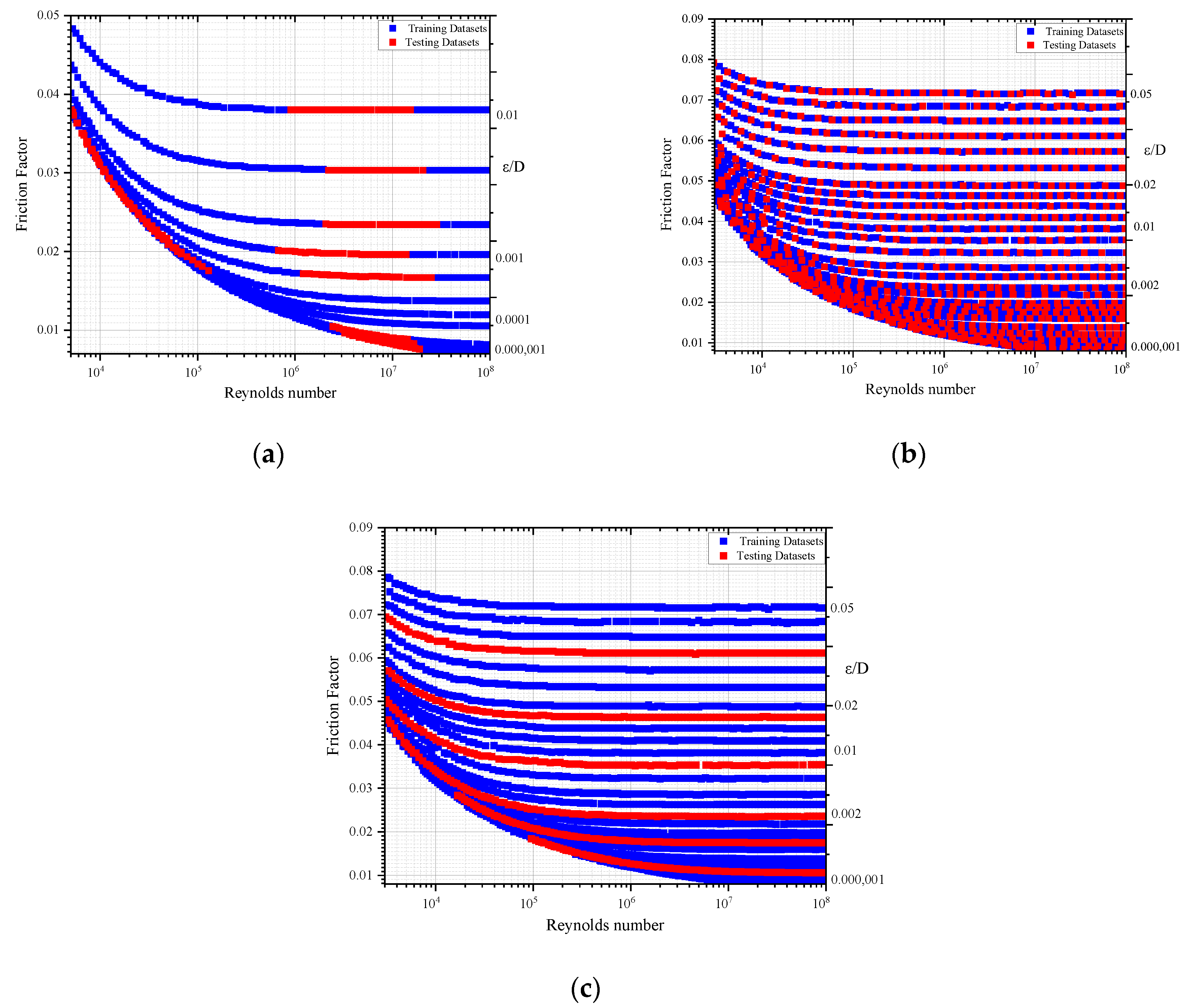
To evaluate the accuracy of the AI-based models in determining the friction factor in pipe flow, Moody’s diagram was used as the observed data. Several attempts were made to make the AI tools understand the nature of the curve and its variations. Three approaches were chosen to train the datasets. In approach-1, the friction factor from Moody’s diagram was collected for a turbulent region in the range of 10−2 ≤ ≤ 10−6 and 5 × 10³ ≤ Re ≤ 108. The purpose was to test the efficiency of the AI tools in capturing the friction factor from Moody’s diagram. Hence, 1052 data points were collected. In approach-1, the data were randomly collected without taking the nature of the curve into consideration. Out the whole dataset, 789 (75% of data) data points were taken for training and 263 were taken for testing of the AI-based models, as shown in Figure 1a.
In approach-2, a wide range of data were collected, including both the transition and turbulent regions of Moody’s diagram. The friction factor from Moody’s chart was collected for the range of 5 × 10⁻² ≤ ≤ 10−6 and 3 × 10³ ≤ Re ≤ 108. For training and testing, 3111 data points were collected. In the 2nd approach, 2332 (75% of data) data points were taken for training and 779 were taken for testing the AI-based models. Here, in approach-2, the data were selected at a particular interval. The graphical presentation of data selection is shown in Figure 1b. In approach-3, different curves with different values were chosen for training and testing of the AI-based models. The purpose of this approach was to make the AI techniques understand the trends of the friction factor with variations in and Re. In approach-3, 2418 (78% of data) data points were taken for training and 693 were taken for testing of the AI-based models. Here, in approach-3, the data were selected at a particular interval with respect to . The graphical presentation of data selection is shown in Figure 1c.
Six AI-based models were selected for analysis, including RF, RT, SVM (POLY, PUK, RBF), M5P, M5Rules, and REPTree. The efficacy of a model in predicting the friction factor in pipe flow was primarily classified according to four basic statistical parameters. For model evaluation in the training and testing datasets, the squared correlation coefficient (R2), root-mean-square error (RMSE), mean absolute error (MAE), and Nash–Sutcliffe efficiency (NSE) as described by McCuen et al. [25] were chosen. The representation of R2, MAE, NSE, and RMSE is as follows:
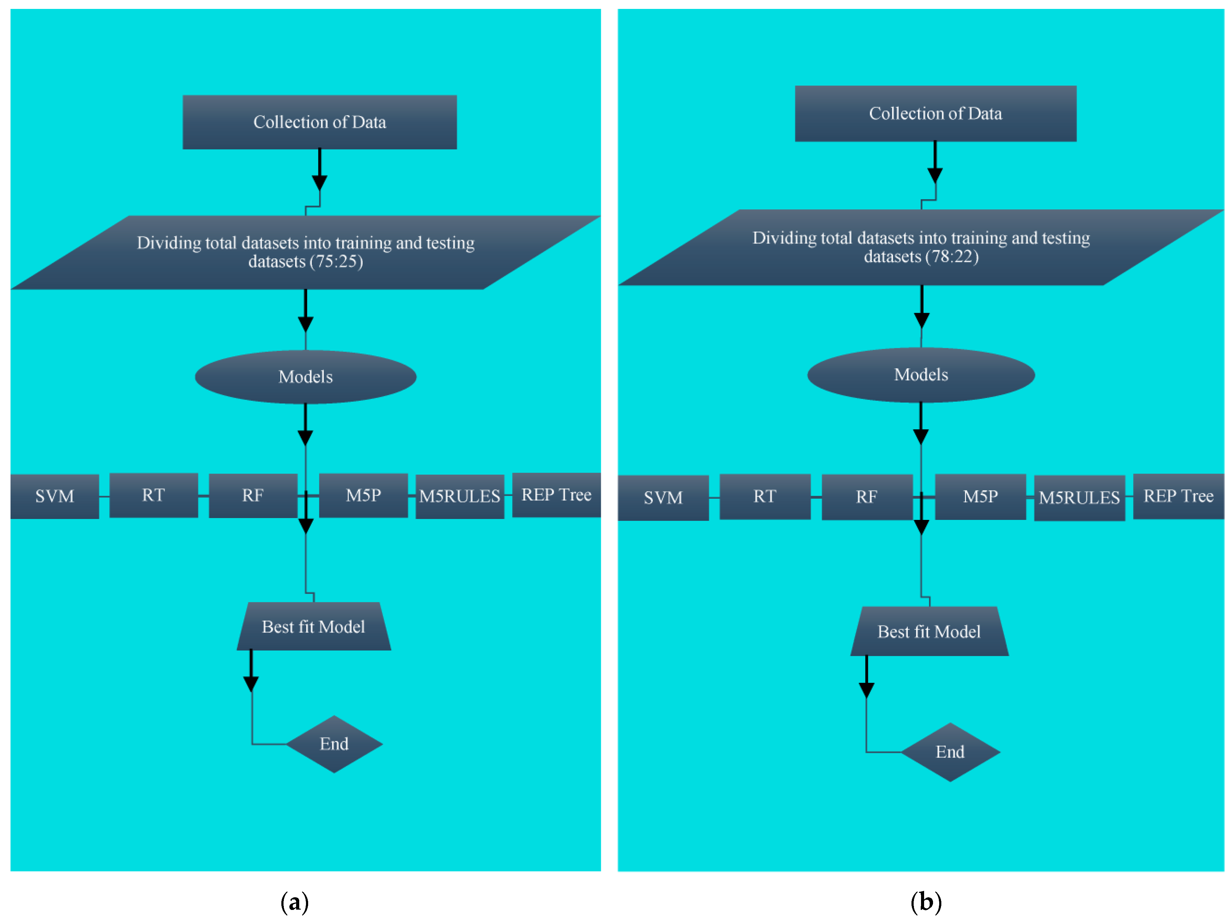
where yobs is the observed data of the friction factor, and y is the simulated friction factor. For better accuracy, the values of R2 and NSE must be close to 1 and those of MAE and RMSE should be close to zero. In modeling the AI tools, the primary work was to collect the data and divide it into training and testing datasets. This was followed by applying different models and choosing the optimal parameters of the models using the hit and trial method. Subsequently, the statistical parameters were evaluated, as mentioned above. In the final stage, the models were ranked as per their performance in predicting accurate results. The process involved in organizing the data, selecting the different models, and choosing the best-fit model as per the statistical parameters is explained in the following flow diagram (Figure 2) in which all three approaches are adopted.
4. Results and Analysis
For predicting the friction factor in pipe flow, six AI-based models, RF, RT, SVM (POLY, PUK, RBF), M5P, M5Rules, and REPTree, were chosen for analysis. Four statistical parameters were selected to evaluate the performance of the model, including RMSE, R2, MAE, and NSE. For each training and testing dataset, the statistical parametric evaluation was performed separately. For the SVM model, the kernel parameters to obtain the optimum predicted values are shown in Table 4. The model performances of the training and testing datasets for approach-1, -2, and -3 are shown in Table 5, Table 6 and Table 7. As per the statistical analysis, the RF model was the most accurate model and ranked 1st among all of the AI-based models, with high R2 and NSE values, as shown in Table 5, Table 6 and Table 7. The RT and REPTree models were ranked as the 2nd and 3rd most accurate models in predicting the friction factor. SVM_POLY was the least accurate model, ranked 8th, with a lower value of R2 during training and testing. For all three approaches, the RF model showed better results as compared to the other AI models based on the statistical analysis.
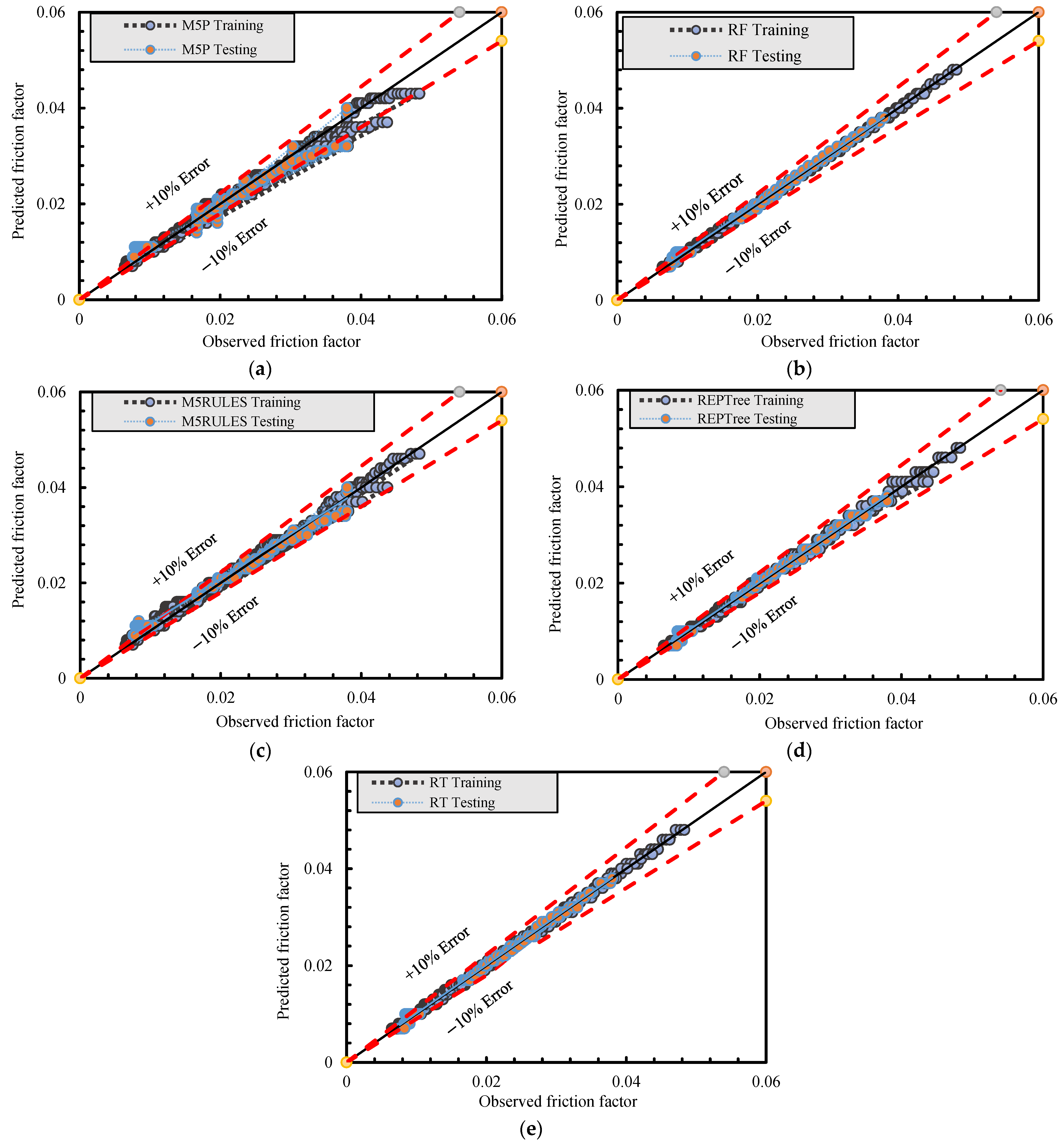
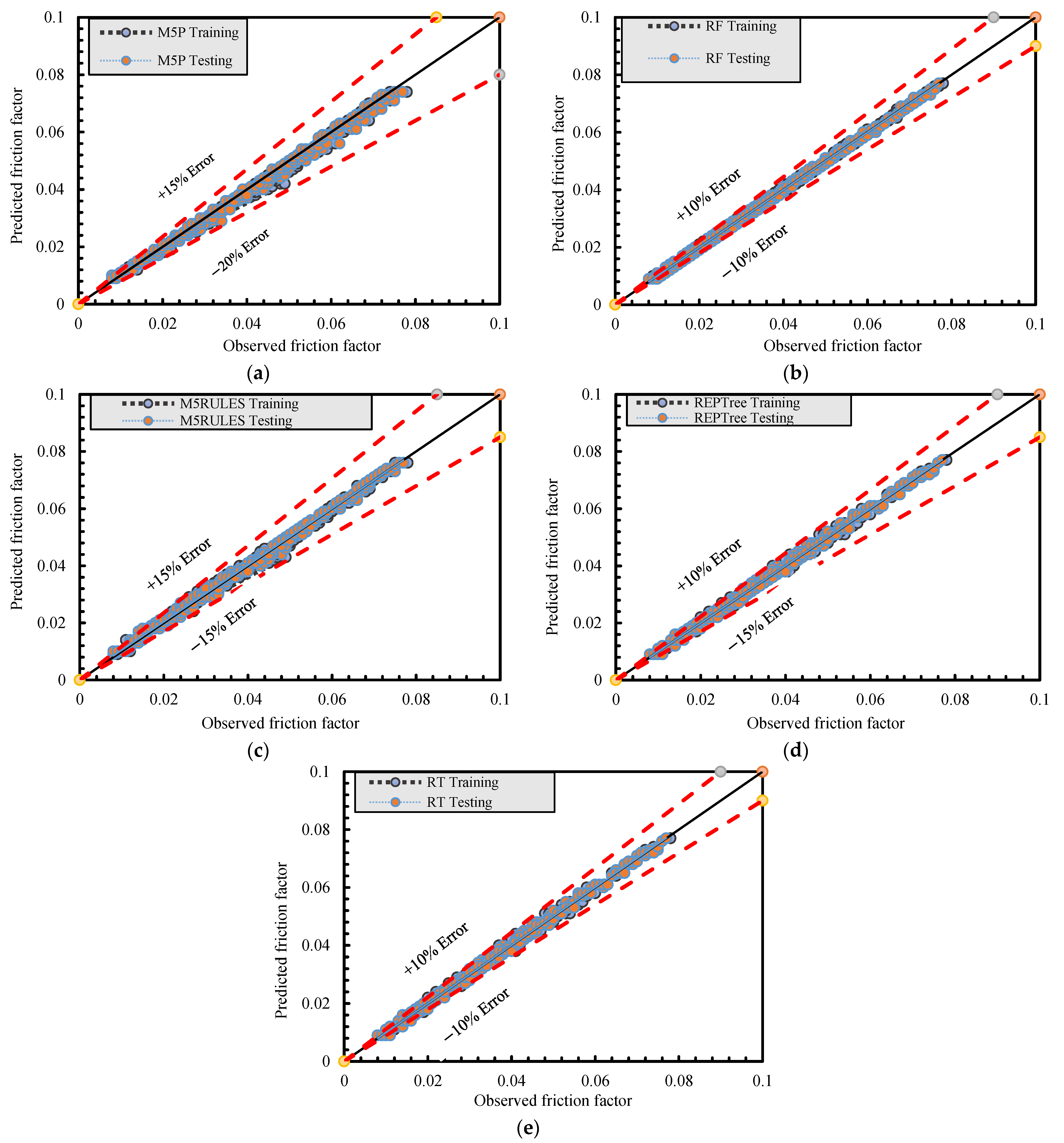
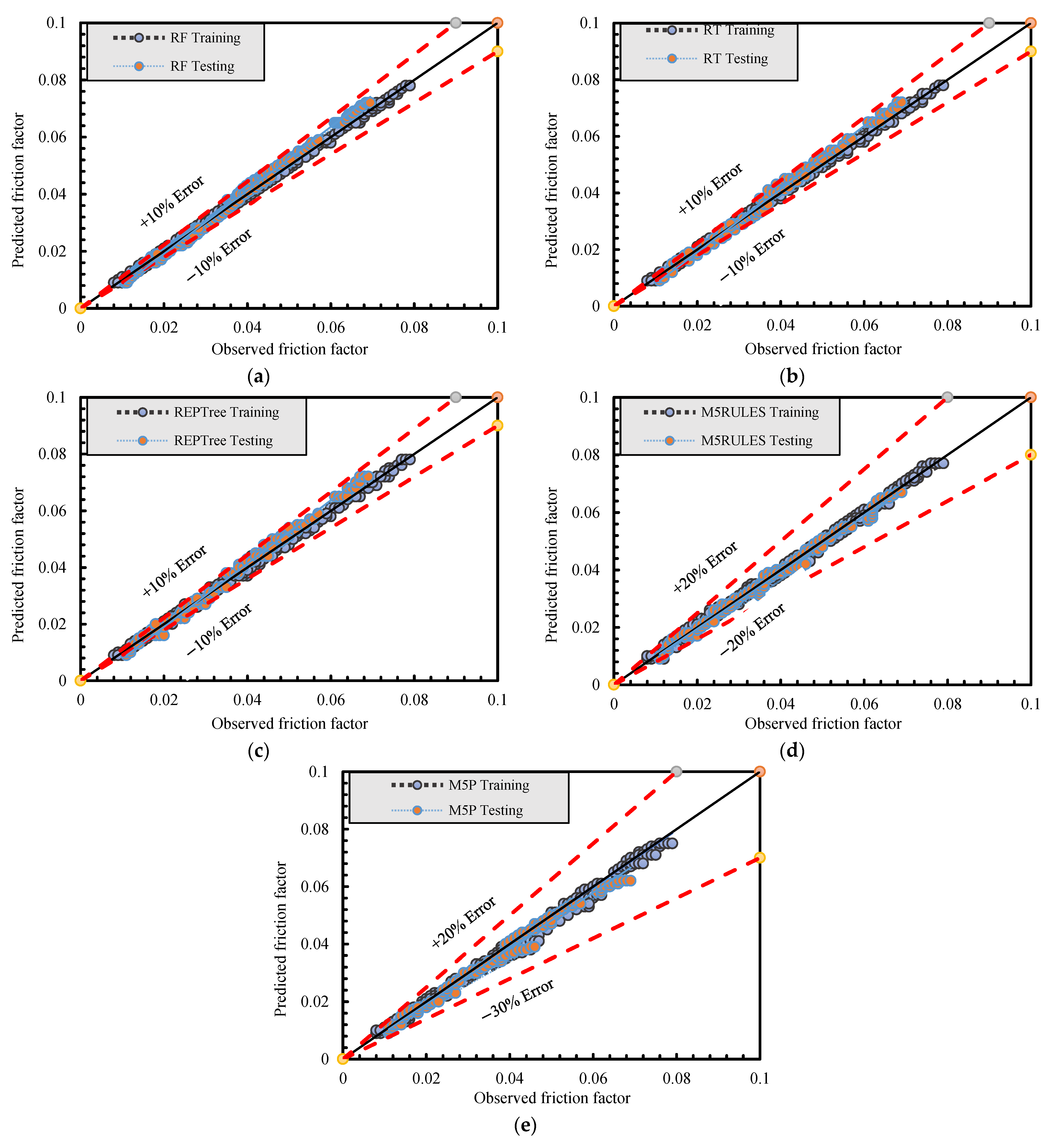
For better visualization, the observed and predicted datasets for approach-1 are represented with the help of an agreement diagram in Figure 3a–e. However, some of the AI models showed a relative error of more than ±35% for approach-1. Likewise, the observed and predicted datasets for approach-2 are represented with the help of an agreement diagram in Figure 4a–e. However, for approach-2, some of the AI models showed a relative error of ±20%. Correspondingly, the observed and predicted datasets for approach-3 are represented with the help of an agreement diagram in Figure 5a–e for all models.
Among all of the AI tools, the RF, RT, and REPTree models predicted well during the training and testing of datasets, whereas the M5P and M5Rules models gave a number of expressions for the solution of friction factor, which are available in Supplementary Material in Tables S3 and S4. Likewise, the tree distribution of the REPTree and RT models are shown in Supplementary Material in Figures S1 and S2. The M5P model gave 49 rules (expressions) to predict the friction factor as per the distribution. Also, the M5Rules model gave 40 rules (expressions) as per the distribution system. However, it is worth noting that both of these models exhibited a relative inaccuracy of around ±30% during testing, as seen in Figure 3, Figure 4 and Figure 5.
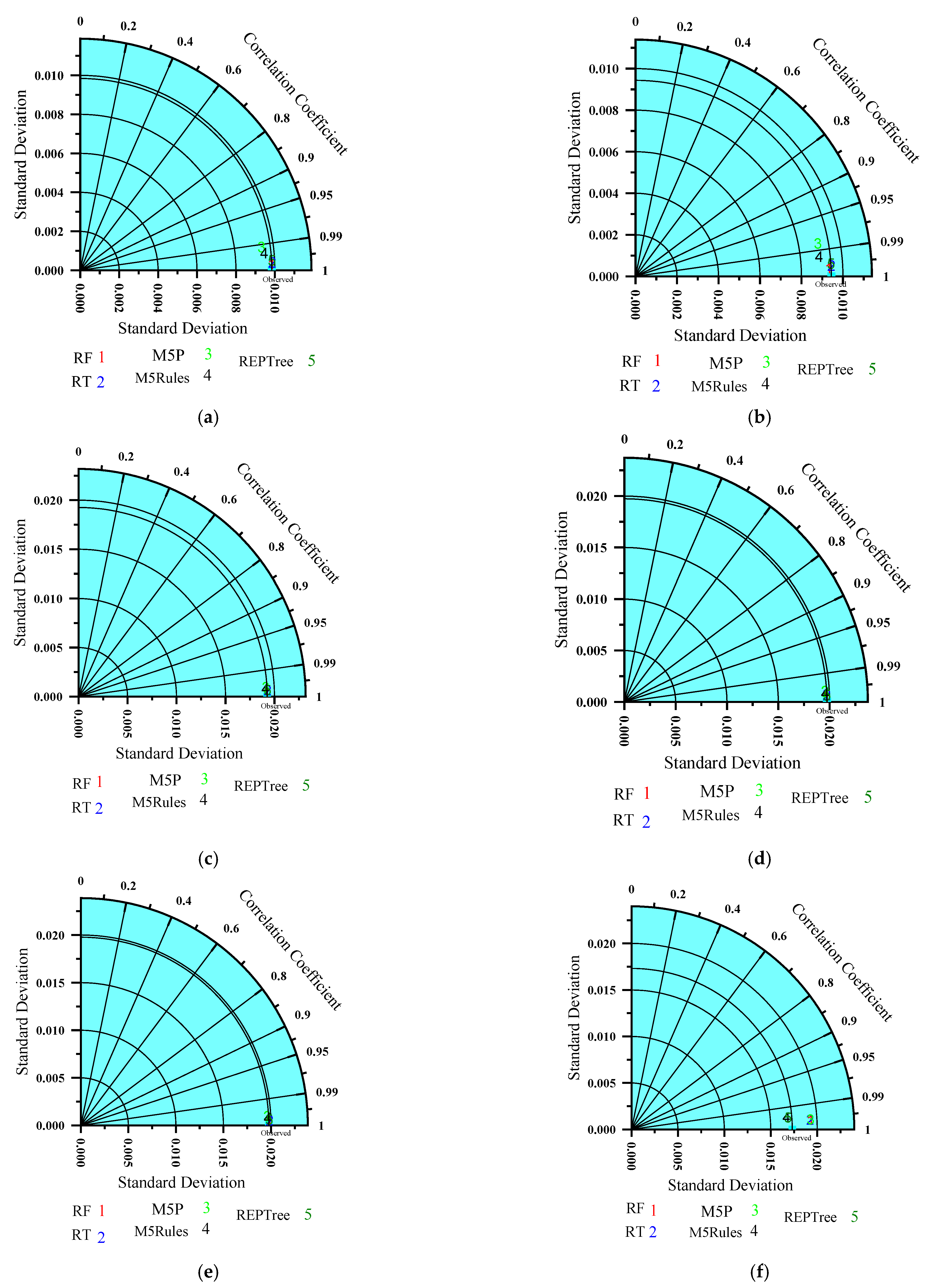
Alternatively, the datasets of the AI-based models could be represented using a Taylor diagram that represented correlation coefficients (CCs) along with standard deviations of all datasets. The Taylor diagrams of all models along with the simulated data for the training and testing datasets for all three approaches are shown in Figure 6a–e. Similar findings were found using the Taylor diagrams. It could be concluded that out of all these AI tools, RF was the most powerful tool for accurately predicting the friction factor in pipe flow.
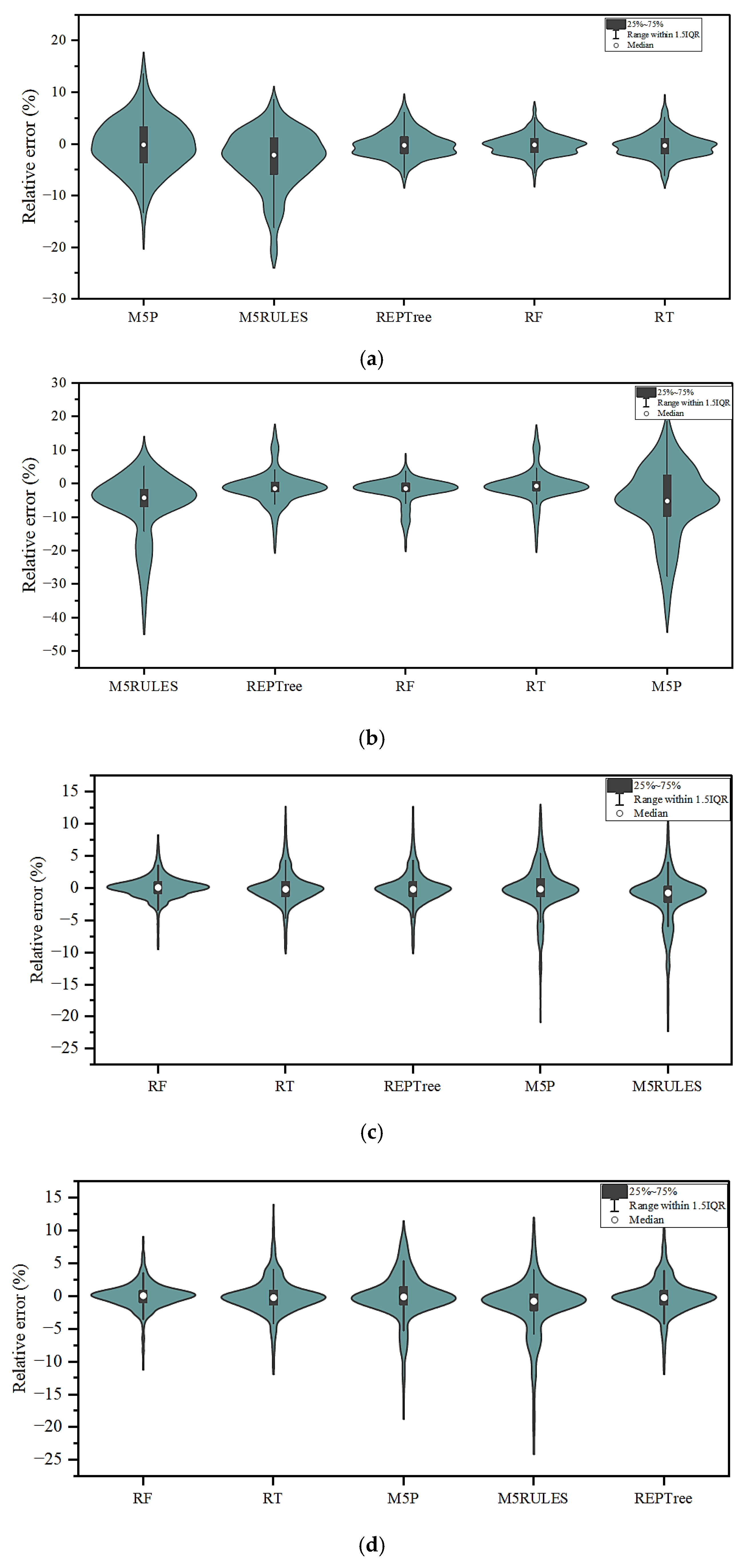
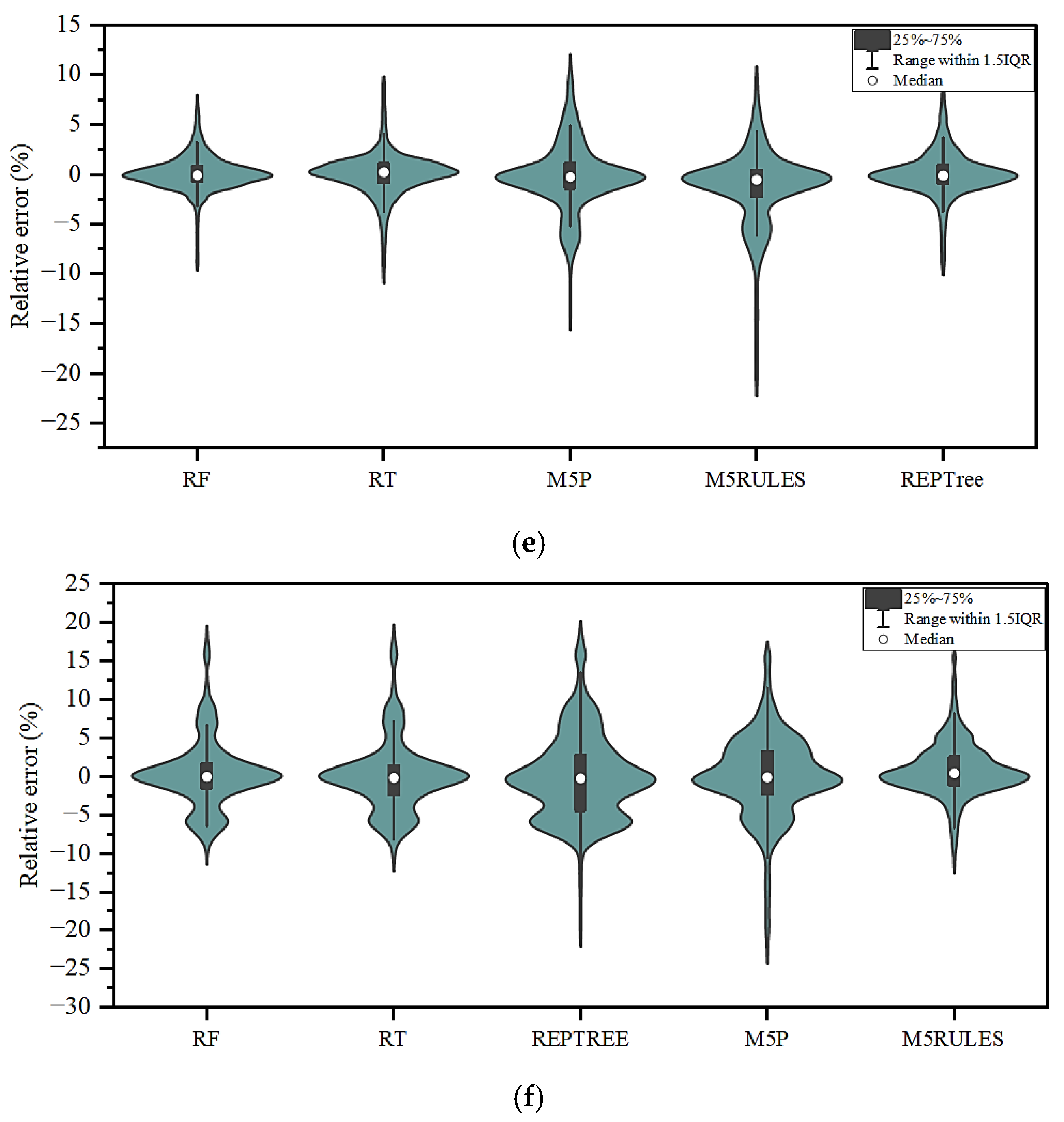
Another aspect of consideration was the determination of the relative error of the observed and predicted datasets. Therefore, the relative errors of all of the predicted datasets from the different AI models are shown in Figure 7. In this part, the training and testing datasets were considered as distinct entities to determine and evaluate their relative error. Figure 7a shows the relative error of the RF, RT, REPTree, M5P, and M5Rules models, which varied ±25% during training. Likewise, Figure 7b displays the relative error of the testing datasets of all models, which varied ±45%. Figure 7c,d displays the relative error of all models for approach-2, with variations of ±25% during both training and testing. Similarly, for approach-3, Figure 7e,f shows a relative error of ±30% for both training and testing.
The research conducted using the three approaches for selecting the data for training and testing confirmed that approach-2 yielded superior results. These three different approaches for training and testing the models were employed to make the AI tool learn the curve of the friction factor and its trends. A substantial percentage of relative error indicated that the AI tool faced difficulties in accurately capturing the friction factor in some region. However, after so many trials, the AI tool failed to capture the trend in the curve in some regions. Thus, it was important to find the region where the RF model failed to accurately capture the value of the friction factor. Hence, it was essential to conduct comprehensive research to identify the specific region among approach-1, -2, and -3 where the accuracy of prediction was somewhat poorer.
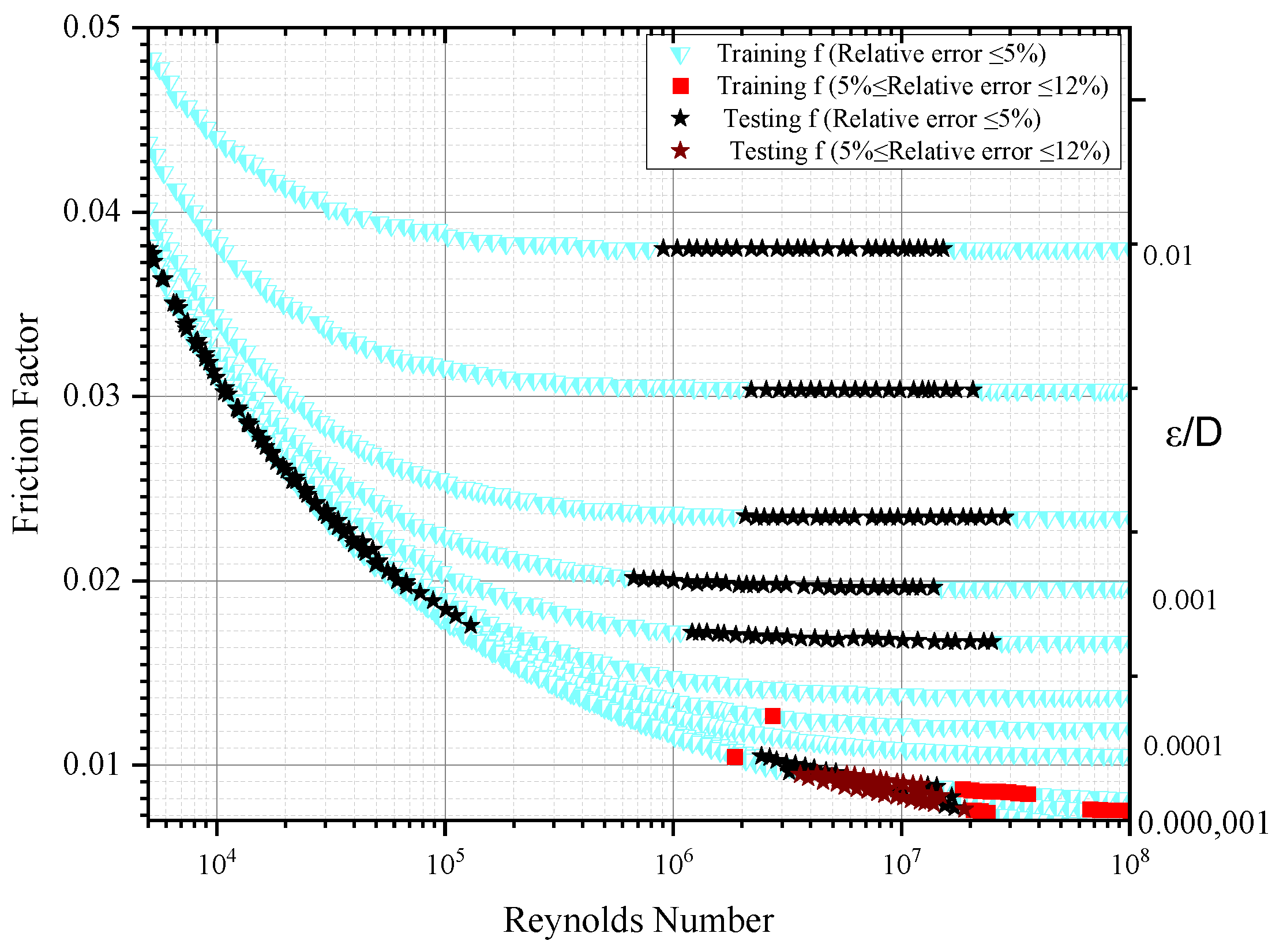
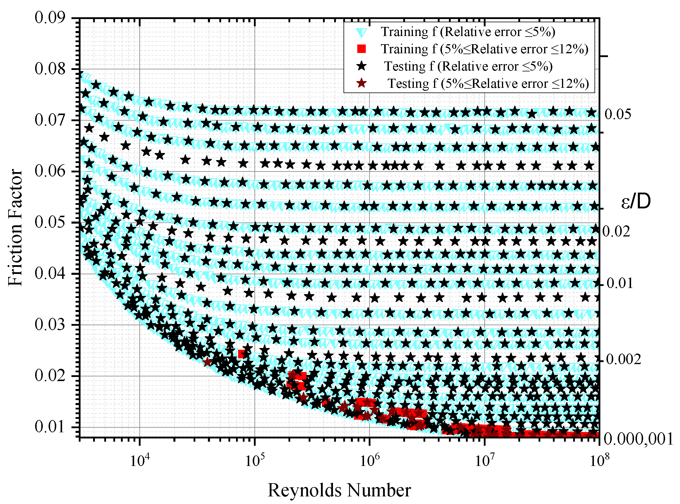
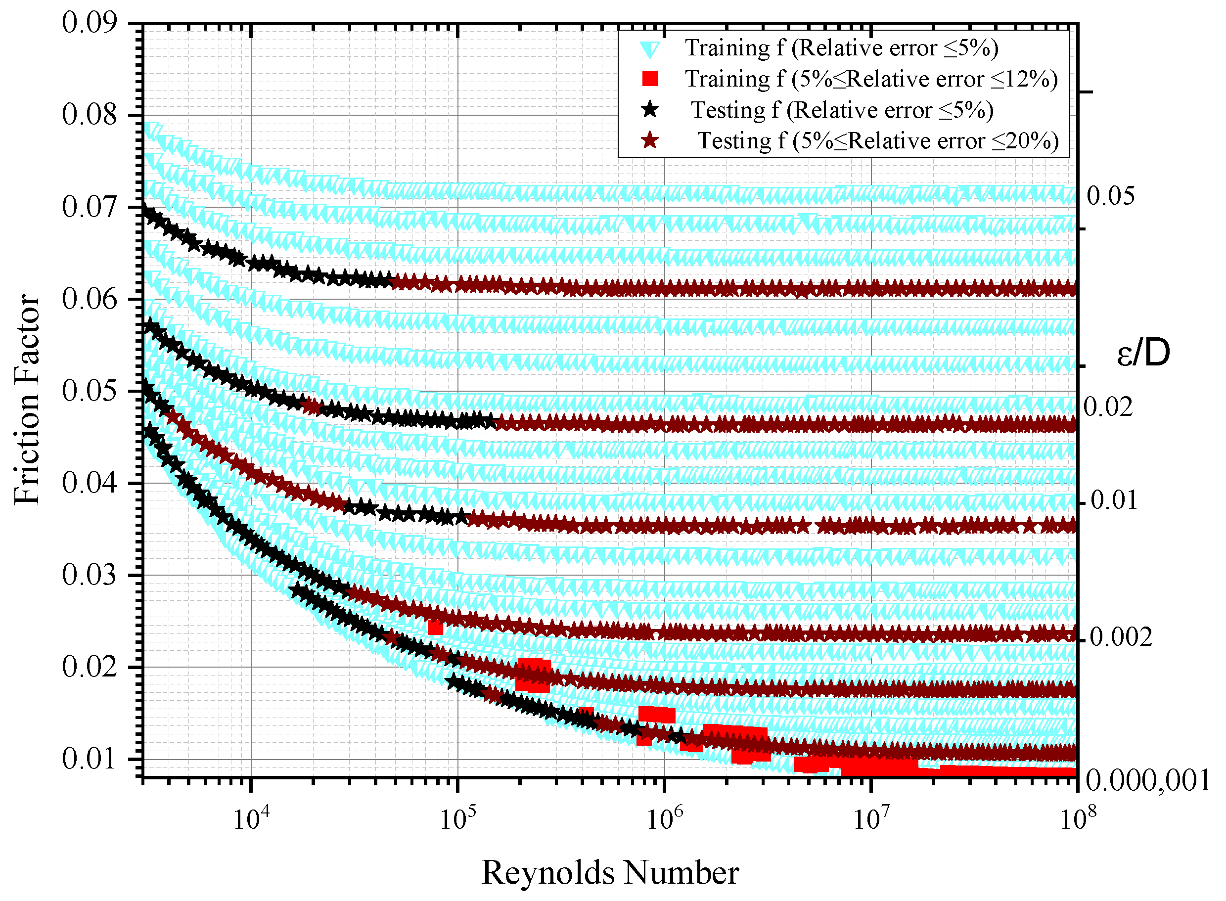
To examine this aspect, the friction factor was plotted in two different segments, such as relative error ≤ 5% and 5% ≤ relative error ≤ 12% for the training and testing datasets of approach-1 and -2. From Figure 8, it can be clearly seen that during training as well as testing, the predicted values were less accurate for the datasets of the turbulent flow region in the range of 3 × 10⁶ ≤ Re ≤ 4 × 10⁷. From Figure 9, it can be seen that during training as well as testing, the predicted values were less accurate in the datasets of the turbulent flow region in the range of 2 × 10⁵ ≤ Re ≤ 108 for approach-2. Likewise, in testing, most of the datasets that failed to be captured by the AI tools were in the range of 3 × 10⁴ ≤ Re ≤ 107. But, in other sections, the AI tools were good enough to capture accurate results. Equally, for approach-3, the friction factor was plotted in two different segments, such as relative error ≤ 5% and 5% ≤ relative error ≤ 12% for training and relative error ≤ 5% and 5% ≤ relative error ≤ 20% for the testing datasets. The approach that exhibited the highest degree of error in data capture during the testing phase was approach-3.
Based on the findings presented in Figure 10, it could be observed that the predicted values for the turbulent flow region were found to be inaccurate throughout the range of 2 × 10⁵ ≤ Re ≤ 108, both in the training and testing datasets. But, in the testing phase, most of the datasets failed to be captured by the AI tools for almost all regions. The testing datasets were unable to capture the variation as well as the trend in the curve and showed a maximum error of 20%. Thus, it could be inferred that the Al tools were not successful in capturing the trends in the friction factor in turbulent regions with higher Reynolds numbers.
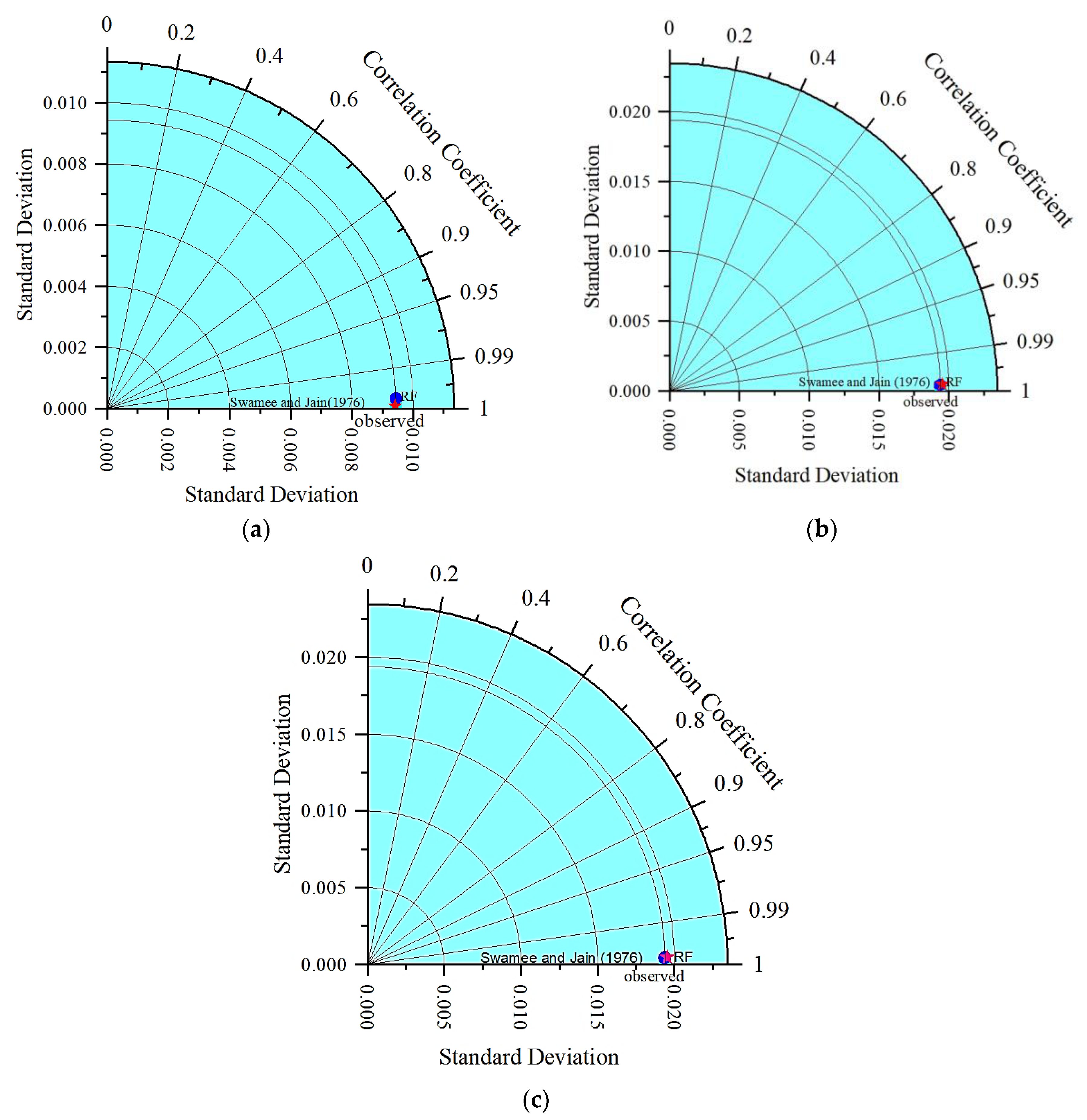
Further, all of the datasets for the three different approaches were compared with the expression given by [8]. The datasets were re-evaluated using the expression given by [8] and compared with the simulated results of the RF model with the help of Taylor’s diagram. Figure 11a–c shows the training and testing datasets of the RF model along with the predicted values from the expression given by [8] for the three different approaches.
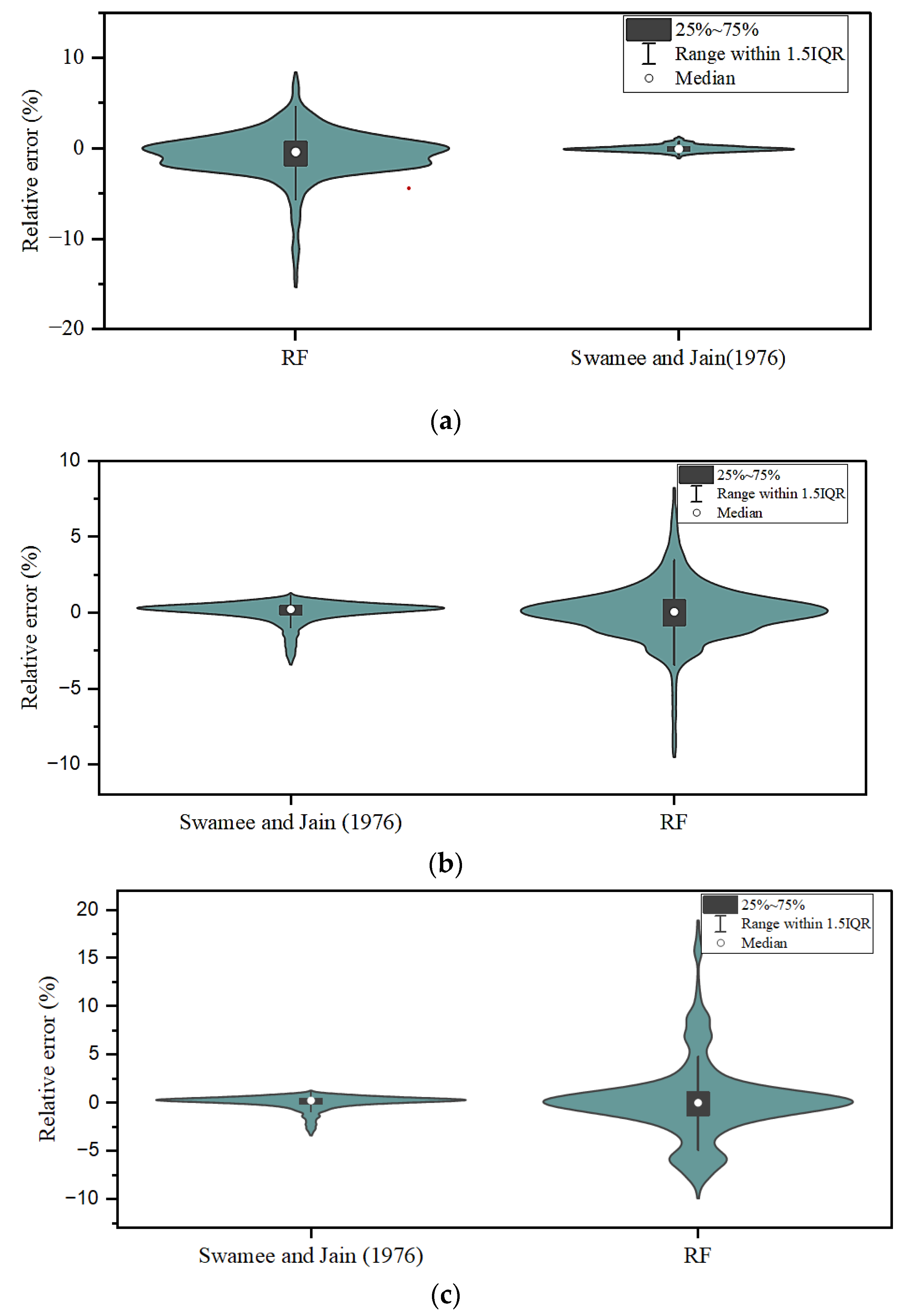
Again, the relative errors using the expression given by [8] and the RF model are compared in Figure 12a–c with the help of a Violin error box diagram. It is clearly seen from Figure 12a–c that the expression given by [8] predicted the friction factor more accurately with a relative error of ≤ ±1% for the turbulent region (approach-1) and 3.5% for both the transition and turbulent regions (approach-2 and -3). From this analysis, it was inferred that the conventional model given by [8] was more appropriate for predicting the friction factor. The performance of the RF model showed inadequacy when compared to the conventional expression provided by [8].
Thus, it can be said that the explicit solution of the Colebrook–White expression given by [8] is one of the most accurate methods and has the potential to predict the friction factor in pipe flow more accurately than modern AI-based techniques. The expression given by [8] is also capable of estimating discharge through the pipe and the diameter of the pipe in turbulent flow regions. Further, the explicit expression given by [8] is one of the earliest methods, and it is heartening to see that it can predict the friction factor more accurately and efficiently than modern techniques. It is worth noting that modern AI techniques like the M5P and M5Rules models gave 49 and 40 expressions to solve the friction factor with an error of ±25% during training.
In contrast, the explicit solution given by [8] can solve the friction factor in a single step with maximum efficiency. The expression given by [8] has the potential to predict the friction factor even more accurately than the solution given by [7] and is claimed to be applicable to different regions of flow, i.e., smooth turbulent regions, rough turbulent regions, and the transition zone of turbulent flow in a pipe. However, the expression given by [7] is not applicable for smooth turbulent regions. Hence, it is essential to realize that while current artificial intelligence (AI) technologies show expertise across multiple scenarios, their limitations in accurately capturing the behavior of the friction factor were observed within specific ranges of the Reynolds number (Re) and relative roughness in the current context.
5. Conclusions
In the present study, a comprehensive analysis of Moody’s diagram was performed using both AI-based models and traditional algebraic expressions discussed in the literature. Various AI-based models, including RF, RT, SVM_POLY, SVM_PUK, SVM_RBF, M5P, M5Rules, and REPTree, were evaluated using Moody’s diagram. Three distinct approaches were chosen to train the AI tools with the objective of enhancing their predictive accuracy. The results highlight the strengths as well as limitations of AI tools when compared to well-established traditional approaches given in the literature. The following conclusions are worth mentioning.
Out of all of the AI models, the Random Forest model had the greatest degree of accuracy in predicting the friction factor throughout both the training and testing phases. In some regions of Moody’s diagram, particularly during the transition of the curve, the AI approaches were not successful in better representing the variations and trends in the curve at different values of in turbulent regions.
It is relevant to note that the Random Forest model had the capability of providing predictions with a relative error of ±12% in some regions of Moody’s diagram. In contrast, the performance evaluation of the explicit solution for the friction factor revealed a relative error of ≤±1%. Based on the analysis, it can be concluded that the used algebraic expression has the ability to predict the friction factor in pipe flow with a relative error of ≤±1% for the range of 10−6 ≤ ≤ 10−2 and 5 × 10³ ≤ Re ≤ 108. It is worth emphasizing that the algebraic expression is a powerful method and has the potential to predict the friction factor in pipe flow with greater accuracy than current AI-based methods in turbulent flow regions.
Thus, the present study provides insight into the use and limitations of AI tools in predicting the friction factor in pipe flow. Better understanding may facilitate further development of models or the integration of hybrid techniques that combine the abilities of AI tools and conventional approaches to predict the friction factor in pipe flow.
Supplementary Materials
The following supporting information can be downloaded at: https://www.mdpi.com/article/10.3390/j6040036/s1, Supplementary: (A) Tree distribution; (B) Comparison of approach-1 results; (C) Tree distribution and expressions. Figure S1: REPTree tree distribution of approach-2; Figure S2: Random Tree distribution of approach-2; Figure S3: M5P distribution of approach-3; Figure S4: Agreement diagram of observed and predicted friction factor of approach-1 by using expression of [8]; Figure S5: Taylor diagram of approach-1 (a) Training, (b) Testing; Figure S6: Violin error box diagram of approach-1 (a) Training, (b) Testing. Table S1: REPTree distribution system of approach-2; Table S2: M5 pruned model tree of approach-2; Table S3: M5 pruned model tree equations of approach-2; Table S4: M5Rules model rules of approach-2.
Author Contributions
Conceptualization, C.S.P.O. and R.M.; methodology, R.M.; software, C.S.P.O.; validation, C.S.P.O., R.M. and C.S.P.O.; formal analysis, R.M.; investigation, R.M.; resources, C.S.P.O.; data curation, R.M.; writing—original draft preparation, C.S.P.O.; writing—review and editing, R.M.; visualization, C.S.P.O.; supervision, C.S.P.O. All authors have read and agreed to the published version of the manuscript.
Funding
This research received no external funding.
Institutional Review Board Statement
Not applicable.
Informed Consent Statement
Not applicable.
Data Availability Statement
All supporting data and models used during this study can be made available from the corresponding author upon reasonable request.
Acknowledgments
C.S.P.O. would particularly like to pay tribute, gratitude, and remembrance to his mentor, the late P.K. Swamee. This article is an invited article and free of processing fee. C.S.P.O. would like to express his thanks to the editors of this special issue. We hope that this article will be able to highlight the great intellectual ability of the late P.K. Swamee without undermining the importance of emerging applications of AI-based tools.
Conflicts of Interest
The authors declare no conflict of interest.
References
- Wang, H.; Xu, Y.; Shi, B.; Zhu, C.; Wang, Z. Optimization and intelligent control for operation parameters of multiphase mixture transportation pipeline in oilfield: A case study. J. Pipeline Sci. Eng. 2021, 1, 367–378. [Google Scholar] [CrossRef]
- Xu, Y.; Wang, Z.; Hong, J.; Zhou, B.; Pu, H. An Insight into Wax Precipitation, Deposition, and Prevention Stratagem of Gas-Condensate Flow in Wellbore Region. J. Energy Resour. Technol. 2023, 145, 093101. [Google Scholar] [CrossRef]
- Colebrook, C.F.; White, C.M. Experiments with Fluid Friction Factor in Roughened Pipes. Proc. R. Soc. Lond. Ser. A 1937, 161, 367–381. [Google Scholar] [CrossRef]
- Colebrook, C.F. Turbulent Flow in Pipes, with Particular Reference to the Transition Region between the Smooth and Rough Pipe Laws. J. Inst. Civ. Eng. 1939, 11, 133–156. [Google Scholar] [CrossRef]
- Moody, L.F. Friction Factors for Pipe Flow. Trans. Am. Soc. Mech. Eng. 1944, 66, 671–681. [Google Scholar] [CrossRef]
- Moody, L.F. An approximate formula for pipe friction factors. Trans. Am. Soc. Mech. Eng. 1947, 69, 1005–1011. [Google Scholar]
- Wood, D.J. An explicit friction factor relationship. Civil. Eng. 1966, 36, 60–61. [Google Scholar]
- Swamee, D.K.; Jain, A.K. Explicit Equations for Pipe Flow Problems. J. Hydraul. Div. 1976, 102, 657–664. [Google Scholar] [CrossRef]
- Swamee, P.K. Design of a submarine oil pipeline. J. Transp. Eng. 1993, 119, 159–170. [Google Scholar] [CrossRef]
- Swamee, P.K.; Swamee, N. Full range pipe-flow equations. J. Hydraul. Res. 2007, 45, 841–843. [Google Scholar] [CrossRef]
- Swamee, P.K.; Sharma, A.K. Design of Water Supply Pipe Networks; John Wiley & Sons, Inc.: Hoboken, NJ, USA, 2008; pp. 11–41. [Google Scholar]
- Swamee, P.K.; Ojha, C.S.P. Drag coefficient and fall velocity of nonspherical particles. J. Hydraul. Eng. 1991, 117, 660–667. [Google Scholar] [CrossRef]
- Kumar, S.; Ojha, C.S.P.; Tiwari, N.K.; Ranjan, S. Exploring the potential of artificial intelligence techniques in prediction of the removal efficiency of vortex tube silt eject. Int. J. Sediment Res. 2023, 38, 615–627. Available online: https://www.sciencedirect.com/science/article/abs/pii/S100162792300015X?via%3Dihub (accessed on 31 March 2023). [CrossRef]
- Breiman, L. Bagging Predictors. Mach. Learn. 1996, 24, 123–140. Available online: https://link.springer.com/content/pdf/10.1023/A:1018054314350.pdf (accessed on 22 September 2023). [CrossRef]
- Breiman, L.; Friedman, J.H.; Olshen, R.A.; Stone, C.J. Classification and Regression Trees; Chapman & Hall: New York, NY, USA, 1984. [Google Scholar] [CrossRef]
- Breiman, L. Using Adaptive Bagging to Debias Regression; Report No. 547; Statistics Department, University of California at Berkeley: Berkeley, CA, USA, 1999. [Google Scholar]
- Vapnik, V. The support vector method of function estimation. In Nonlinear Modeling; Springer: Boston, MA, USA, 1998; pp. 55–85. Available online: https://link.springer.com/chapter/10.1007/978-1-4615-5703-6_3 (accessed on 22 September 2023).
- Han, S.; Qubo, C.; Meng, H. Parameter selection in SVM with RBF kernel, function. In Proceedings of the World Automation Congress, Puerto Vallarta, Mexico, 24–28 June 2012; IEEE: Piscataway, NJ, USA, 2012; pp. 1–4. [Google Scholar]
- Sihag, P.; Jain, P.; Kumar, M. Modelling of impact of water quality on recharging rate of stormwater filter system using various kernel function-based regression. Model. Earth Syst. Environ. 2018, 4, 61–68. Available online: https://link.springer.com/article/10.1007/s40808-017-0410-0 (accessed on 22 September 2023). [CrossRef]
- Smola, A.J.; Sch€olkopf, B. A tutorial on support vector regression. Stat. Comput. 2004, 14, 199–222. Available online: https://link.springer.com/article/10.1023/B:STCO.0000035301.49549.88 (accessed on 22 September 2023). [CrossRef]
- Quinlan, J.R. Learning with continuous classes. In Proceedings of the 5th Australian Joint Conference on Artificial Intelligence, Hobart, Tasmania, 16–18 November 1992; Volume 92, pp. 343–348. [Google Scholar]
- Holmes, G.; Hall, M.; Prank, E. Generating rule sets from model trees. In Lecture Notes in Computer Science; Springer: Berlin/Heidelberg, Germany, 1999. [Google Scholar] [CrossRef]
- Ayaz, Y.; Kocamaz, A.F.; Karakoç, M.B. Modeling of compressive strength and UPV of high-volume mineral-admixtured concrete using rule-based M5 rule and tree model M5P classifiers. Constr. Build. Mater. 2015, 94, 235–240. [Google Scholar] [CrossRef]
- Rajesh, P.; Karthikeyan, M. A Comparative study of data mining algorithms for decision tree approaches using WEKA tool. Am. Eurasian Netw. Sci. Inf. 2017, 11, 230–241. [Google Scholar]
- McCuen, R.H.; Knight, Z.; Cutter, A.G. Evaluation of the nashi-sutcliffe efficiency index. J. Hydrol. Eng. 2006, 11, 597–602. [Google Scholar] [CrossRef]
Figure 1.
Selection of training and testing datasets of Moody’s diagram for the friction factor in pipe flow. (a) Approach-1; (b) Approach-2; (c) Approach-3.
Figure 1.
Selection of training and testing datasets of Moody’s diagram for the friction factor in pipe flow. (a) Approach-1; (b) Approach-2; (c) Approach-3.

Figure 2.
Flow diagram of predicting the friction factor for (a) approach-1 and -2; (b) approach-3.

Figure 3.
Agreement diagram of observed and predicted friction factors of training and testing datasets for approach-1. (a) M5P model; (b) RF model; (c) M5Rules model; (d) REPTree model; (e) RT model.
Figure 3.
Agreement diagram of observed and predicted friction factors of training and testing datasets for approach-1. (a) M5P model; (b) RF model; (c) M5Rules model; (d) REPTree model; (e) RT model.

Figure 4.
Agreement diagram of observed and predicted friction factors of training and testing datasets for approach-2. (a) M5P model; (b) RF model; (c) M5Rules model; (d) REPTree model; (e) RT model.
Figure 4.
Agreement diagram of observed and predicted friction factors of training and testing datasets for approach-2. (a) M5P model; (b) RF model; (c) M5Rules model; (d) REPTree model; (e) RT model.

Figure 5.
Agreement diagram of observed and predicted friction factors of training and testing datasets for approach-3. (a) RF model; (b) RT model; (c) REPTree model; (d) M5rules model; (e) M5P model.
Figure 5.
Agreement diagram of observed and predicted friction factors of training and testing datasets for approach-3. (a) RF model; (b) RT model; (c) REPTree model; (d) M5rules model; (e) M5P model.

Figure 6.
Taylor diagrams of AI models RF, RT, REPTree, M5P, and M5Rules. (a) Training datasets for approach-1; (b) Testing datasets for approach-1; (c) Training datasets for approach-2; (d) Testing datasets for approach-2; (e) Training datasets for approach-3; (f) Testing datasets for approach-3.
Figure 6.
Taylor diagrams of AI models RF, RT, REPTree, M5P, and M5Rules. (a) Training datasets for approach-1; (b) Testing datasets for approach-1; (c) Training datasets for approach-2; (d) Testing datasets for approach-2; (e) Training datasets for approach-3; (f) Testing datasets for approach-3.

Figure 7.
Violin error box diagrams. (a) Training datasets of all models for approach-1; (b) Testing datasets of all models for approach-1; (c) Training datasets of all models for approach-2; (d) Testing datasets of all models for approach-2; (e) Training datasets of all models for approach-3; (f) Testing datasets of all models for approach-3.


Figure 8.
Relative error for approach-1 during training and testing.

Figure 9.
Relative error for approach-2 during training and testing.

Figure 10.
Relative error for approach-3 during training and testing.

Figure 11.
Taylor diagram of training and testing datasets for (a) approach-1; (b) approach-2; (c) approach-3 [8].
Figure 11.
Taylor diagram of training and testing datasets for (a) approach-1; (b) approach-2; (c) approach-3 [8].

Figure 12.
Violin error box diagrams of training and testing datasets for (a) approach-1; (b) approach-2; (c) approach-3.
Figure 12.
Violin error box diagrams of training and testing datasets for (a) approach-1; (b) approach-2; (c) approach-3.


Table 1.
Expressions of friction factor described in the literature.
| Reference | Expression | Condition | Flow Type |
|---|---|---|---|
| [3,4] | Re ≥ 4000 | Turbulent flow | |
| [6] | ≤ 10−2 4 × 10³ ≤ Re ≤ 107 | Turbulent flow | |
| [7] | ≤ 4 × 10⁻² 4 × 10³ ≤ Re ≤ 5 × 10⁷ | Turbulent flow | |
| [8] | Smooth turbulent flow | ||
| [8] | Rough turbulent flow | ||
| [8] | ≤ 10−2 5 × 10³ ≤ Re ≤ 108 | Transition zone of turbulent flow | |
| [9] | All regions | ||
| [9] | Turbulent flow |
Table 2.
Expressions of discharge in the pipe flow described in the literature.
| Reference | Expression (m3/s) | Condition |
|---|---|---|
| [8] | Turbulent region | |
| [10] | All regions |
Table 3.
Expressions of diameter of the pipe described in the literature.
| Reference | Expression (m) | Condition |
|---|---|---|
| [8] | Turbulent region | |
| [10] | All regions |
Table 4.
User-defined parameters of models.
| Method | User-Defined Parameter Training and Testing |
|---|---|
| SVM-POLY | C = 10, d = 3.6 |
| SVM-RBF | C = 10, d = 4.8 |
| SVM-PUK | C = 10, ω = 1.7, σ = 1 |
Table 5.
Performance of models for the training dataset in approach-1.
| Method | R2 Training | RMSE | MAE | NSE | Ranking | R2 Testing | RMSE | MAE | NSE |
|---|---|---|---|---|---|---|---|---|---|
| RF | 0.9998 | 0.0001 | 0.0001 | 0.9989 | 1 | 0.9990 | 0.0004 | 0.0003 | 0.9971 |
| RT | 0.9992 | 0.0003 | 0.0002 | 0.9983 | 2 | 0.9972 | 0.0005 | 0.0004 | 0.9967 |
| REPTree | 0.9982 | 0.0004 | 0.0003 | 0.9973 | 3 | 0.9970 | 0.0005 | 0.0004 | 0.9952 |
| M5Rules | 0.9926 | 0.001 | 0.0008 | 0.9892 | 4 | 0.9892 | 0.0014 | 0.0012 | 0.9793 |
| M5P | 0.9854 | 0.0013 | 0.0009 | 0.9822 | 5 | 0.9706 | 0.0017 | 0.0015 | 0.9641 |
| SVM-PUK | 0.7793 | 0.0049 | 0.0029 | 0.7522 | 6 | 0.6798 | 0.0062 | 0.0039 | 0.5616 |
| SVM-RBF | 0.6266 | 0.0061 | 0.0047 | 0.6161 | 7 | 0.4881 | 0.0068 | 0.0051 | 0.4751 |
| SVM-POLY | 0.6255 | 0.0061 | 0.0046 | 0.6098 | 8 | 0.4881 | 0.007 | 0.0053 | 0.4397 |
Table 6.
Performance of models for the training and testing datasets in approach-2.
| Method | R2 Training | RMSE | MAE | NSE | Ranking | R2 Testing | RMSE | MAE | NSE |
|---|---|---|---|---|---|---|---|---|---|
| RF | 0.9998 | 0.0003 | 0.0003 | 0.9995 | 1 | 0.9996 | 0.0004 | 0.0003 | 0.9994 |
| RT | 0.9992 | 0.0006 | 0.0004 | 0.9989 | 2 | 0.9990 | 0.0006 | 0.0004 | 0.9988 |
| REPTree | 0.9992 | 0.0006 | 0.0004 | 0.9989 | 3 | 0.9990 | 0.0006 | 0.0004 | 0.9988 |
| M5Rules | 0.9984 | 0.0008 | 0.0006 | 0.9979 | 4 | 0.9984 | 0.0008 | 0.0006 | 0.9979 |
| M5P | 0.9978 | 0.0009 | 0.0006 | 0.9974 | 5 | 0.9978 | 0.0009 | 0.0006 | 0.9974 |
| SVM-PUK | 0.9731 | 0.0033 | 0.0017 | 0.9713 | 6 | 0.9735 | 0.0032 | 0.0018 | 0.9732 |
| SVM-RBF | 0.9204 | 0.0056 | 0.0041 | 0.9152 | 7 | 0.9191 | 0.0056 | 0.0041 | 0.9192 |
| SVM-POLY | 0.8877 | 0.0065 | 0.0053 | 0.8855 | 8 | 0.8862 | 0.0065 | 0.0053 | 0.8894 |
Table 7.
Performance of models for the training and testing datasets in approach-3.
| Method | R2 Training | RMSE | MAE | NSE | Ranking | R2 Testing | RMSE | MAE | NSE |
|---|---|---|---|---|---|---|---|---|---|
| RF | 0.9998 | 0.0003 | 0.0003 | 0.9995 | 1 | 0.9972 | 0.0024 | 0.0021 | 0.9816 |
| RT | 0.9996 | 0.0004 | 0.0003 | 0.9993 | 2 | 0.9968 | 0.0024 | 0.0021 | 0.9814 |
| REPTree | 0.9994 | 0.0005 | 0.0004 | 0.9991 | 3 | 0.9968 | 0.0024 | 0.0022 | 0.9810 |
| M5Rules | 0.9986 | 0.0008 | 0.0006 | 0.9983 | 4 | 0.9952 | 0.0015 | 0.0011 | 0.9807 |
| M5P | 0.9978 | 0.0009 | 0.0006 | 0.9975 | 5 | 0.9950 | 0.0019 | 0.0014 | 0.9806 |
| SVM-PUK | 0.9753 | 0.0032 | 0.0018 | 0.9732 | 6 | 0.9692 | 0.0032 | 0.0017 | 0.9518 |
| SVM-RBF | 0.9250 | 0.0056 | 0.0041 | 0.9195 | 7 | 0.9101 | 0.0054 | 0.0039 | 0.9033 |
| SVM-POLY | 0.8903 | 0.0066 | 0.0054 | 0.8887 | 8 | 0.8847 | 0.0061 | 0.0048 | 0.8746 |
Disclaimer/Publisher’s Note: The statements, opinions and data contained in all publications are solely those of the individual author(s) and contributor(s) and not of MDPI and/or the editor(s). MDPI and/or the editor(s) disclaim responsibility for any injury to people or property resulting from any ideas, methods, instructions or products referred to in the content. |
© 2023 by the authors. Licensee MDPI, Basel, Switzerland. This article is an open access article distributed under the terms and conditions of the Creative Commons Attribution (CC BY) license (https://creativecommons.org/licenses/by/4.0/).
Share and Cite
MDPI and ACS Style
Mishra, R.; Ojha, C.S.P. Application of AI-Based Techniques on Moody’s Diagram for Predicting Friction Factor in Pipe Flow. J 2023, 6, 544-563. https://doi.org/10.3390/j6040036
AMA Style
Mishra R, Ojha CSP. Application of AI-Based Techniques on Moody’s Diagram for Predicting Friction Factor in Pipe Flow. J. 2023; 6(4):544-563. https://doi.org/10.3390/j6040036
Chicago/Turabian StyleMishra, Ritusnata, and Chandra Shekhar Prasad Ojha. 2023. "Application of AI-Based Techniques on Moody’s Diagram for Predicting Friction Factor in Pipe Flow" J 6, no. 4: 544-563. https://doi.org/10.3390/j6040036