
Multiplicity Analysis of a Thermistor Problem—A Possible Explanation of Delamination Fracture

Institute of Thermal Research, 2 Kanigos Str, P.O. Box 106 77 Athens, Greece
J 2023, 6(3), 517-535; https://doi.org/10.3390/j6030034
Submission received: 27 June 2023
/
Revised: 20 August 2023
/
Accepted: 27 August 2023
/
Published: 4 September 2023
Abstract
:In the present study, a numerical bifurcation analysis of a PTC thermistor problem is carried out, considering a realistic heat dissipation mechanism due to conduction, nonlinear temperature-dependent natural convection, and radiation. The electric conductivity is modeled as a strongly nonlinear and smooth function of the temperature between two limiting values, based on measurements. The temperature field has been resolved for both cases were either the current or the voltage (nonlocal problem) is the controlling parameter. With the aid of an efficient continuation algorithm, multiple steady-state solutions that do not depend on the external circuit have been identified as a result of the inherent nonlinearities. The analysis reveals that the conduction–convection parameter and the type of the imposed boundary conditions have a profound effect on the solution structure and the temperature profiles. For the case of current control, depending on the boundary conditions, a complex and interesting multiplicity pattern appears either as a series of nested cusp points or as enclosed branches emanating from pitchfork bifurcation points. The stability analysis reveals that when the device edges are insulated, only the uniform solutions are stable, namely, one “cold” and one “hot”. A key feature of the “hot” state is that the corresponding temperature is proportional to the input power and its magnitude could be one or even two orders of magnitude higher than the “cold” one. Therefore, the change over from the “cold” to the “hot” state induces a thermal shock and could perhaps be the reason for the mechanical failure (delamination fracture) of PTC thermistors.
1. Introduction
Thermistors are thermally sensitive resistors and have either a negative (NTC) or positive (PTC) resistance/temperature coefficient. We will only discuss the latter, albeit certain similarities and differences, especially for the flash sintering phenomenon, will be addressed in the appropriate sections. Its characteristic feature is the strongly dependent electric conductivity. PTCs are manufactured from silicon, barium, lead, and strontium titanates with the addition of yttrium, manganese, tantalium, and silica [1,2,3,4,5]. PTC thermistors are widely used as current-limiting devices, that is, as non-destructible (resettable) fuses for electric circuit protection, sensing excessive currents. They can also be encountered as a micro self-heating thermostat for microelectronic, biomedical, and chemical applications. Common geometrical configurations are the washer, the disk, and the rod type [1,2,3]. Although PTCs and in general electroceramics are, in principle, loaded electrically, a significant number of mechanical failures are recorded annually. This may be explained on the basis of the Joule self-heating effect, which causes temperature differences, thermal strains, and excessive thermo-mechanical stresses that may cause the failure of the device. As the current technological trends point towards greater device miniaturization while operating at higher power densities, there is an increasing demand for a thorough analysis and understanding of the underlying coupled electrothermal phenomena in electroceramic devices (Dewitte et al. [6], Supancic [7], Danzer et al. [8]).
The thermistor, as a coupled thermo-electric problem, has attracted significant attention. An early result (1900) described by Diesselhorst [9] for the steady-state problem shows that the temperature may be expressed as a function of the electric potential provided that certain types of boundary conditions are imposed. Cimatti [10] extended the result of Diesselhorst to obtain existence and uniqueness conditions for the steady-state problem. Further results on existence and uniqueness were obtained by Cimatti [11], Cimatti and Prodi [12], Xie and Allegretto [13], and Antontsev and Chipot [14]. Bahadir [15,16] and Çatal [17] employed finite element numerical techniques to solve the thermistor problem assuming a step electric conductivity function. Kutluay et al. [18] obtained a heat balance integral solution of the same problem considering a modified electric conductivity function. Ammi and Torres [19] numerically solved a nonlocal parabolic equation in time and space domains resulting from the thermistor problem. Golosnoy and Sykulski [20] compared various computational techniques for coupled nonlinear thermo-electric problems. The thermistor problem was used as a test case with an electric conductivity being a nonlinear function of the temperature and the electric field intensity. Karpov [21] demonstrated the bistability conditions, the switching autowave properties, and the emergence of dissipative structures of essentially a thermistor problem under current control. Apart from the temperature-dependent electric conductivity, convective heat dissipation with a constant heat transfer coefficient over the lateral surface was assumed. It is worth noting that the thermistor problem is closely associated with the flash sintering of ceramics [22] such as, for instance, yttria-stabilized zirconia, magnesia-doped alumina, and strontium titanate, among others [23]. The essence of the process is that when an operating parameter such as the furnace temperature exceeds the corresponding limit point, established by the applied voltage that separates the stable from the unstable steady states—the Joule heating greatly exceeds the heat dissipation mechanism due to radiation and the temperature increases significantly. The process controller is then switched from voltage to current control to maintain the temperature within the specified limits [24,25].
From the literature review above, it appears that the thermistor problem has been studied with various assumptions and/or restrictions related primarily to the form of electrical conductivity, the heat dissipation mechanism, and, in certain cases, with the influence of the external electric circuit. The latter is also associated with the existence of multiple steady-state solutions, up to three, as determined from the number of intersection points between the current–voltage characteristic curves of the external (linear) circuit and the thermistor (Fowler et al. [26], Howison et al. [27], Zhou and Westbrook [28], Cimatti [29]). The aim of the present study is to provide a reasonable explanation for the most common reason PTC thermistors fail—namely, delamination fracture due to excessive thermal loading (shock). To this end, a one-dimensional PTC device model based on nonlinear electric resistivity combined with a distributed heat dissipation mechanism due to conduction, nonlinear temperature-dependent natural convection, and radiation has been developed. The problem formulated in this way admits multiple steady-state solutions that do not depend on the external circuit. The numerical bifurcation analysis reveals that the PTC thermistor is a bistable system that can operate between a “cold” and a “hot” stable state. The changeover from the “cold” to the “hot” state induces a kind of thermal shock that could be a reason for potential failure, since the “hot” state is associated with a very high temperature. This hypothesis is further supported by a similar behavior that is encountered in other bistable systems such as superconductors and boiling wires. Depending on the boundary conditions, a complex and interesting multiplicity pattern appears either as a series of nested cusp points or as enclosed branches emanating from pitchfork bifurcation points.
2. Analysis
2.1. Energy Balance
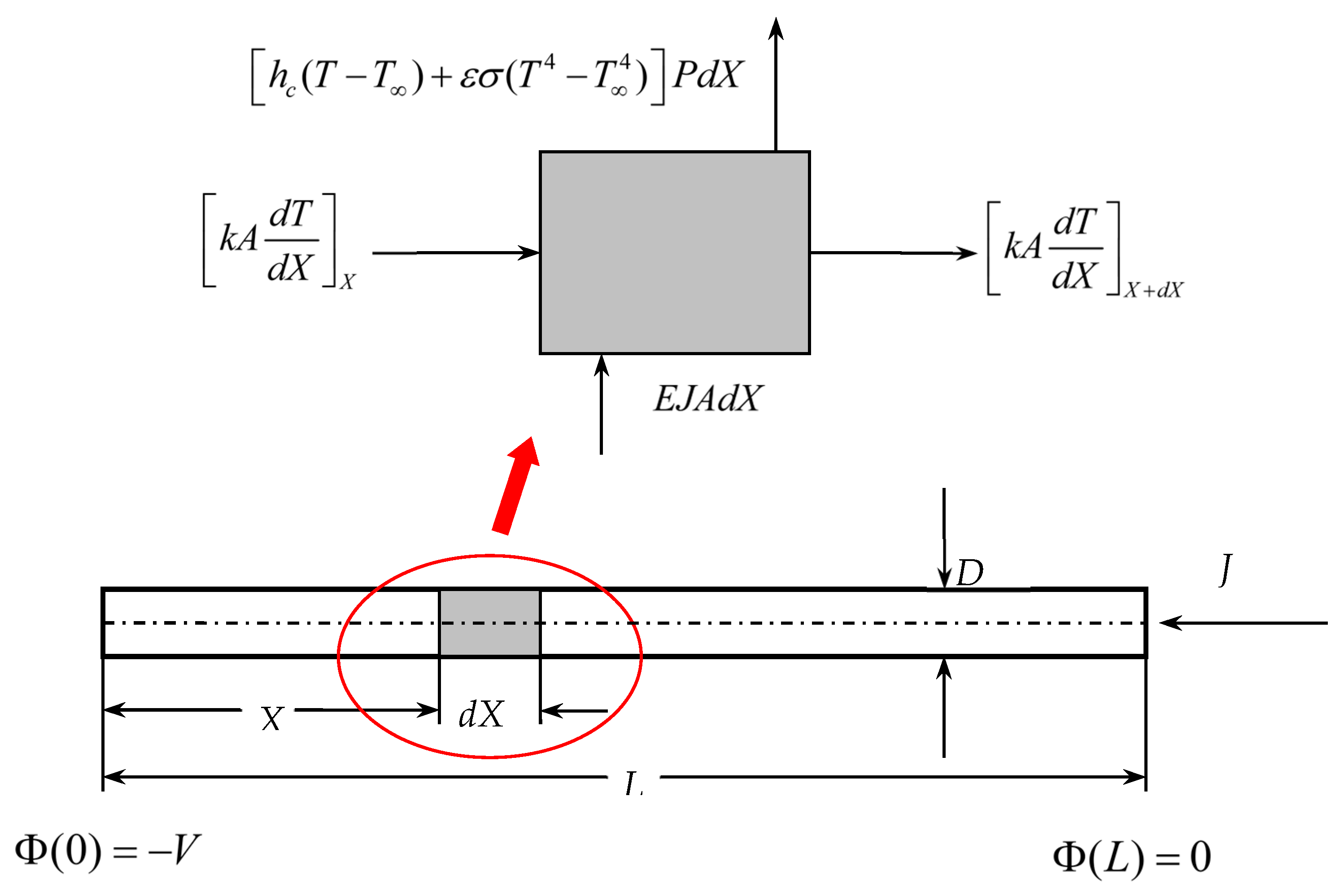
Consider a horizontal cylindrical segment of a conductor of uniform material density γ with constant thermal conductivity k. The segment has a diameter D and length L, as schematically shown in Figure 1. Heat is being dissipated by conduction through the core of the device and by natural convection and radiation through the lateral surface area, in an ambient environment of constant temperature . An energy balance along the longitudinal direction X yields the following partial differential equation for the device temperature T:
Here, C is the specific heat capacity, A is the cross-sectional area, P is the perimeter, is the convective heat transfer coefficient, ε is the surface emissivity, σ is the Stefan–Boltzmann constant, E is the electric field intensity, and J is the current density through the device. Considering a constant (dc) current flowing through the device, the electric field intensity is related to the current density through Ohm’s law, (Metaxas [30], Lupi [31], Lupi et al. [32]). Thus, when the current is controlled, Equation (1) reads:
On the other hand, in many practical applications, the applied voltage across the device is the controlling parameter. This may be taken into account by introducing the electric potential , as in [33]:
Integrating the above relationship and considering that the current remains constant, albeit still unknown, yields:
where V is the voltage drop across the device, as shown in Figure 1. Substituting the current density J from Equation (4) into Equation (2), the energy balance for voltage control takes the form:
Compared with the current control problem, this is a nonlocal problem, since the solution depends on the resistivity integral over the device.
2.2. Electric Resistivity
A characteristic feature of a ceramic PTC device is the strongly nonlinear dependence of its resistivity with respect to temperature. Driven by a transition of the ferroelectric PTC material, the resistance increases several orders of magnitude in a relatively small temperature interval—for instance, between 100 °C and 200 °C. The same smooth curve with continuous derivatives with respect to temperature for the subsequent numerical bifurcation analysis has been adopted from Karpov [21], which represents a barium titanate (BaTiO3)-based device:
where Ωm and Ωm are the asymptotic resistivity values corresponding to the low and high operating temperatures, respectively. The temperature of 95 °C signifies the onset of the transition from the low to the high resistivity value as the contribution of the exponential term in Equation (6) becomes significant. The form of Equation (6) is supported by a significant volume of measurements, as, for instance, those reported by Brzozowski and Castro [34], Wang et al. [35], Wang et al. [36], Luo et al. [37], Takeda et al. [38], and Rowlands and Vaidhyanathan [39].
2.3. Heat Transfer Model
The heat generated in the device due to the current flow (Metaxas [30], Lupi [31], Lupi et al. [32]) is dissipated to the surrounding environment through natural convection and radiation exchange. For the circumferential average Nusselt number Nu, the correlation of Churchill and Chu [40] is employed:
where is a weak function of the Prandtl number Pr. Equation (7) covers a very wide range of Rayleigh numbers, namely, in the range from 10−6 to 109, while it maintains a simple and compact mathematical form. Equation (7) is applied locally in the evaluation of the convective heat transfer coefficient along the device axis (see Figure 1), in a similar manner as it was utilized by Faghri and Sparrow [41]. Consequently, the local Rayleigh number, Ra, is evaluated from the local temperature difference as:
where g is the acceleration due to gravity, β is the thermal expansivity, D is the device diameter, α is the thermal diffusivity, and ν is the kinematic viscosity.
2.4. Boundary Conditions: Problems P1 and P2
As will be described in the next paragraphs, the boundary conditions have a profound effect on the bifurcation structure in general and on the temperature distribution in particular. Thus, for problem P1, the edges of the device are considered adiabatic:
whereas for problem P2, the imposed symmetrical boundary conditions are:
2.5. Electrothermal Model in Dimensionless Form
Introducing dimensionless variables
the temperature distribution along the device takes the form of
for current control and
for voltage control. In the above equations, u is the conduction–convection parameter (CCP), which is extensively used in conjugate heat transfer and electro-thermal problems associated with superconductors and metallic conductors as well [42,43,44], and is defined as:
where the reference heat transfer coefficient is conveniently defined through the Nusselt number:
In terms of the dimensionless variables defined above, the local Rayleigh number becomes:
The current density parameter is related to the current density as below:
and is the ratio of the radiative heat transfer coefficient to the reference heat transfer coefficient
Under steady-state conditions, the partial differential Equation (12) reduces to a two-point boundary value problem for current control:
and, similarly, Equation (13) for the voltage control:
where
The voltage–current relationship becomes
and the boundary conditions are
for problem P1 and
for problem P2. Convenient reference values have been adopted for the electric resistivity and the applied voltage
2.6. Stability
The stability of a certain steady-state to small perturbations i.e.,
is determined by the eigenvalues λ of the corresponding Sturm–Liouville problem, after substituting Equation (22) into the original partial differential equation, Equation (12):
where
The corresponding boundary conditions for problem P1 are and for problem P2 are . During branch tracing, for every steady state that has been calculated from Equation (12), the associated eigenvalue problem, Equation (23), is subsequently numerically solved and a sufficient number of eigenvalues is determined. Stable solutions are characterized by negative eigenvalues, whereas positive ones correspond to unstable temperature distributions.
3. Results and Discussion
The second-order, two-point boundary value problem described by Equation (17) for current control and Equation (18) for voltage control are transformed into a system of first-order equations through the transformation , and solved numerically. In order to ensure an accurate and reliable numerical solution, two different methods have been employed, resulting in identical results under the strict tolerances imposed. The first one utilizes a multi-shooting Runge–Kutta formula pair of order 8(7) (Hairer et al. [45]) and the second one uses a spline collocation method described by Ascher et al. [46]. Continuation along the various branches has been carried out along the lines suggested by Seydel [47]. For the computation of the singular points, an extended problem is formed from the partial derivatives of Equations (17) and (18) with respect to the parameters, according to Witmer et al. [48].
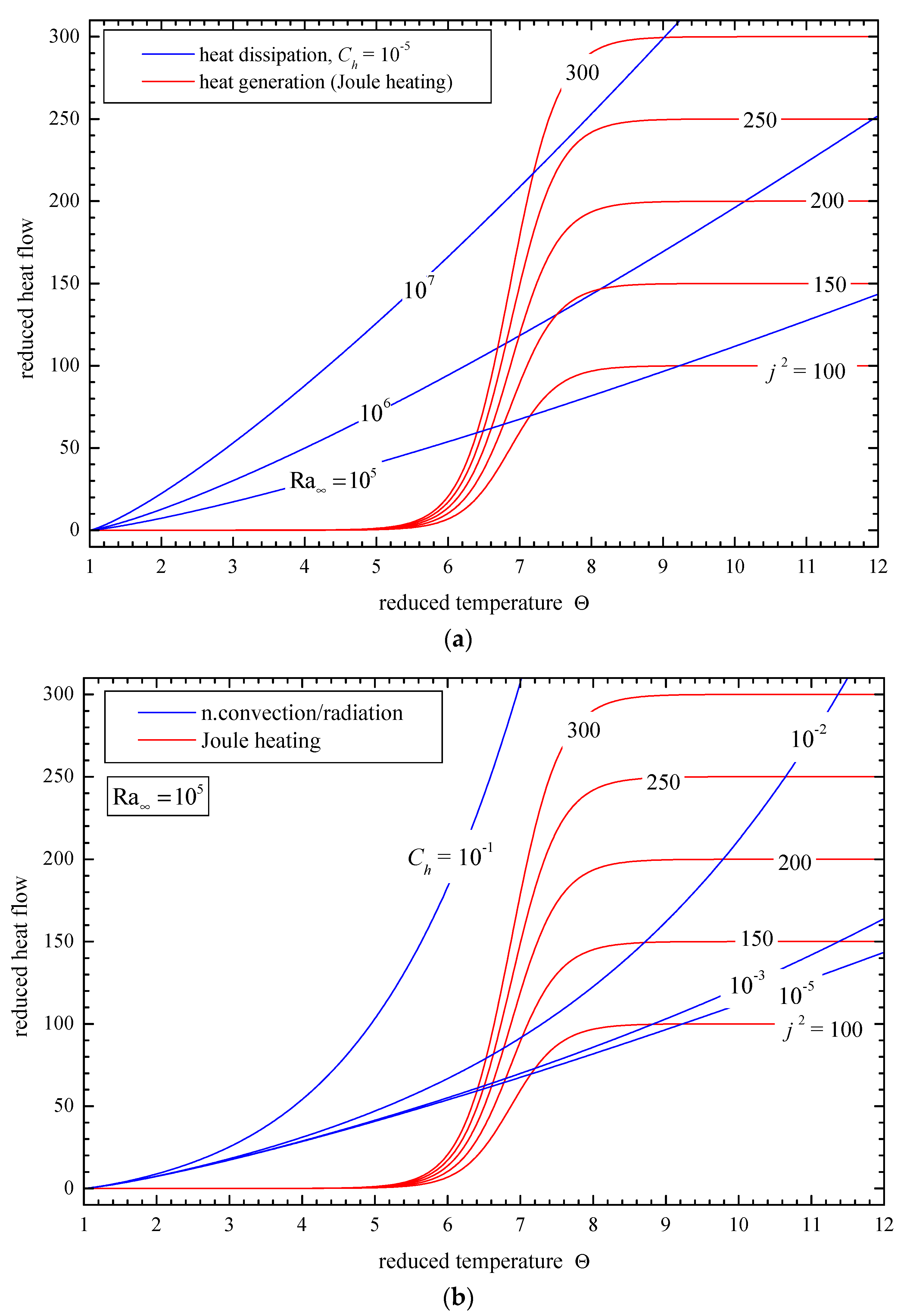
Before we analyze the complete numerical solution, it is instructive to first discuss the uniform solutions of Equation (17), which reduces to an algebraic one for a constant temperature profile:
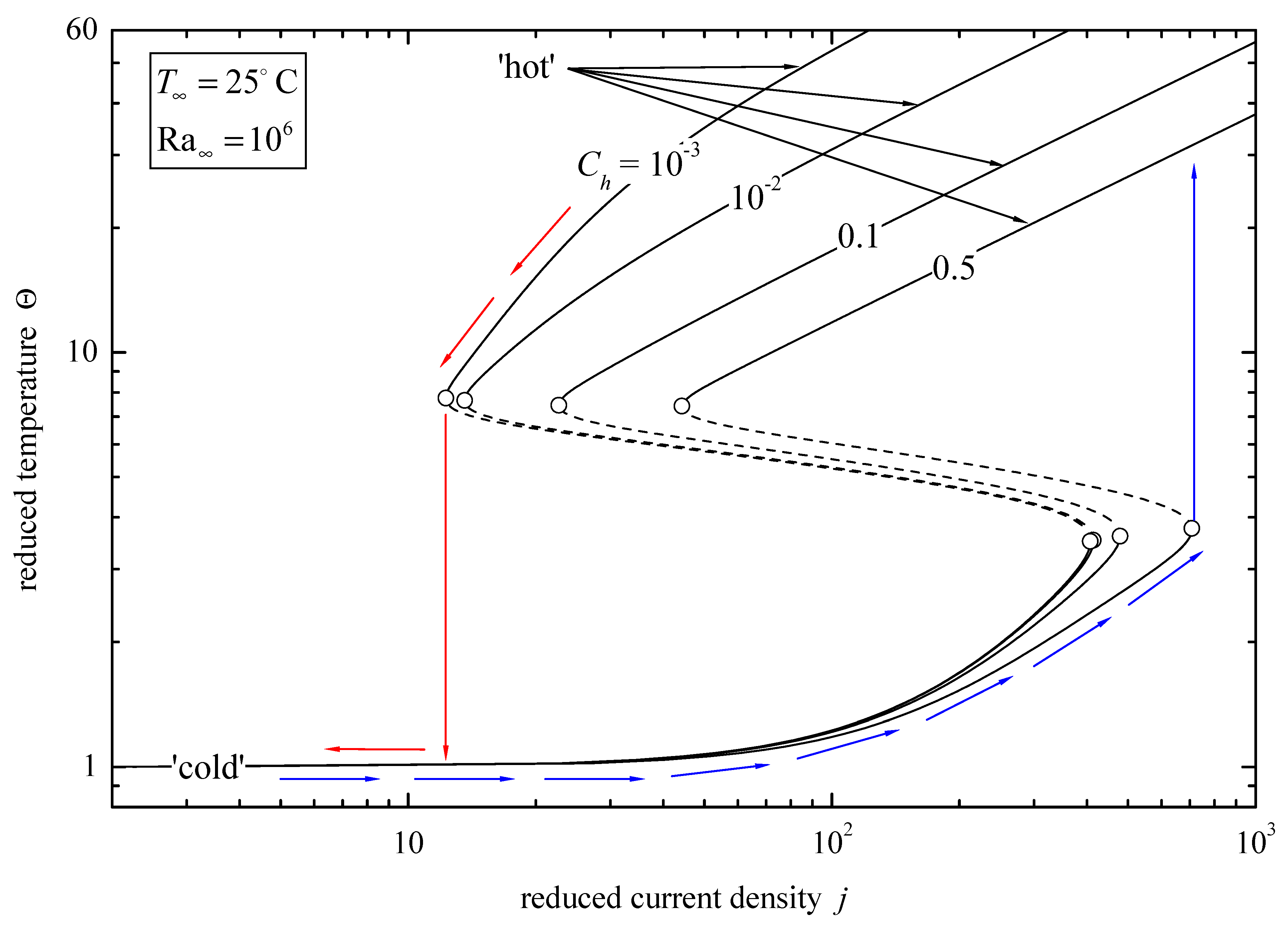
A geometrical (graphical) solution is depicted in Figure 2, where the heat generation and the heat dissipation curves are plotted for a variety of current parameters and reference Rayleigh numbers (Figure 2a). In Figure 2b, the effect of radiation through on the heat rejection rate is demonstrated. Depending on the combination of , and , up to three solutions of Equation (24) may be obtained from the number of the intersection points between the heat generation and the heat dissipation curves, as shown in Figure 3. Three uniform solutions exist: two are stable, namely, the “cold” and the “hot”, whereas the third one at an intermediate temperature is unstable. From this simplified analysis, a few important observations may be pointed out. The “cold” temperature remains practically constant and very close to the ambient temperature for a wide range of current densities. On the other hand, the “hot” temperature appears proportional to the input power (i.e., ), since at this temperature range, the electric resistivity approaches its maximum value, i.e., . Consequently, the “hot” temperature can increase one and even two orders of magnitude compared to the “cold” one. Thus, when a current instability or disturbance gradually propagates through the circuit and the limit point to right is exceeded, as schematically shown in Figure 3, then the “hot” state prevails, and depending on the operating conditions, a significantly higher temperature will be established even if the radiation contribution is significant. This is also known as a hysteresis loop, and under these circumstances, it closely resembles thermal shock. However, this is not a thermal runaway, as is the case during flash sintering, since the temperature could be excessive, but it is still bounded. Therefore, it is reasonable to assume that the bistability (“hot”–“cold”) and the associated hysteresis loop could be a potential reason for the mechanical failure (i.e., delamination fracture; Dewitte et al. [6], Supancic [7], Danzer et al. [8]) of PTC thermistors. In practice, however, the conditions prevailing could worsen either due to the dense packing of the electronic devices or because of poor cooling. This inevitably will shift the “hot” temperature even higher.
3.1. Current Control Problem P1
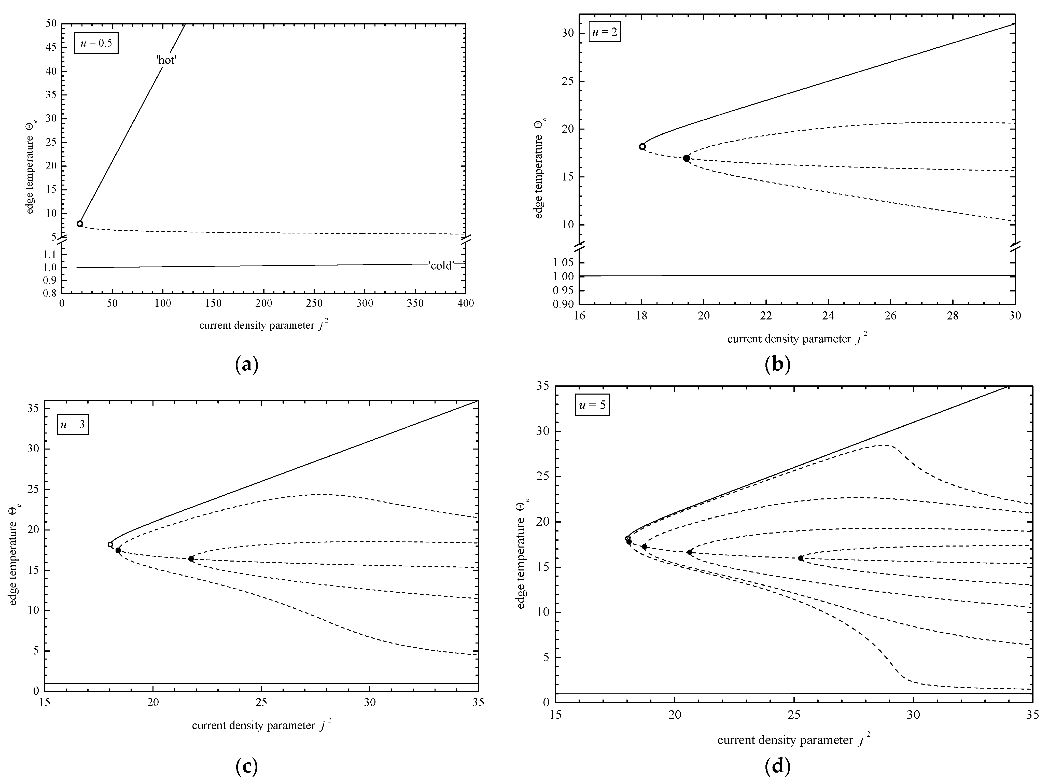
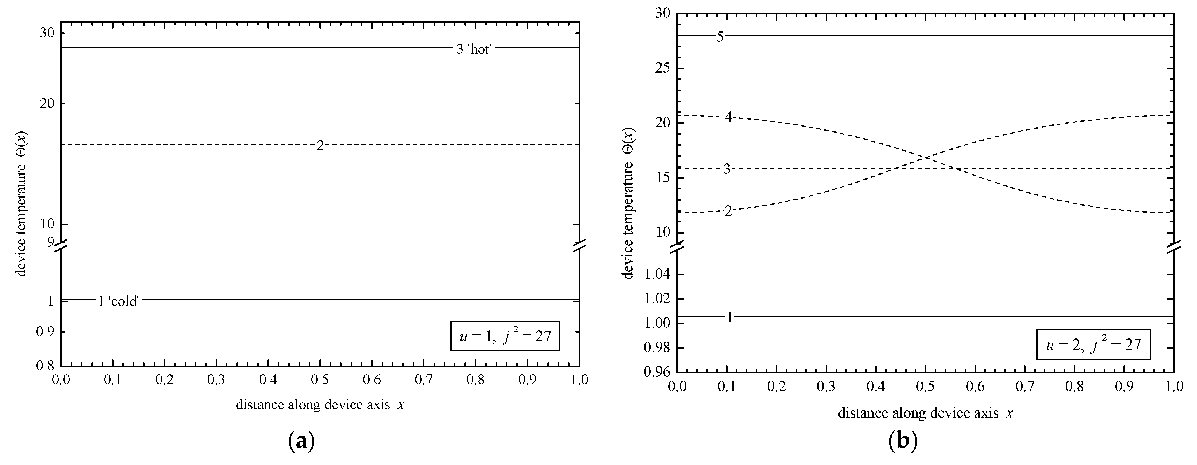
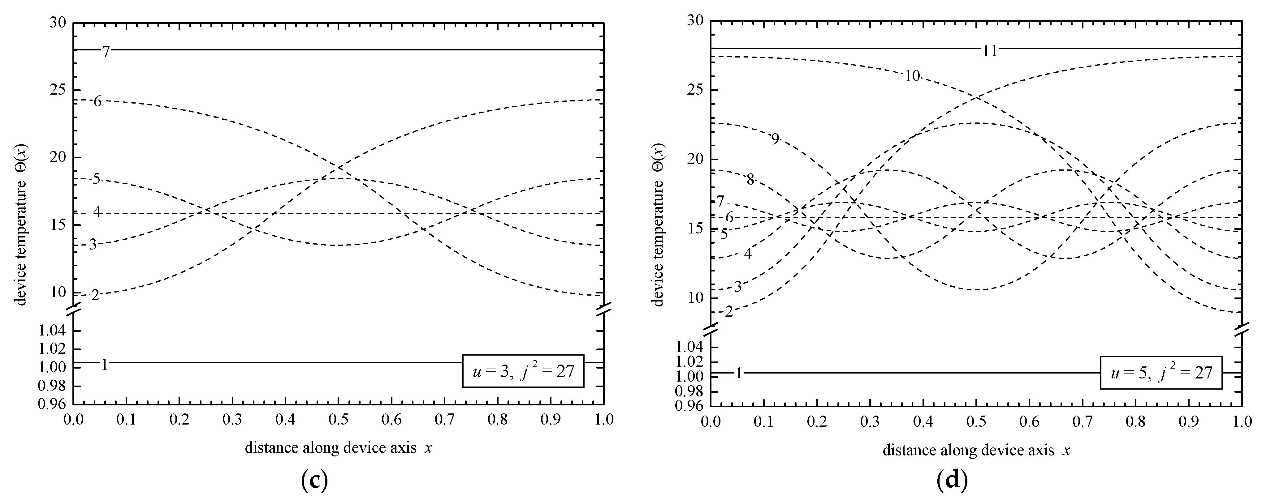
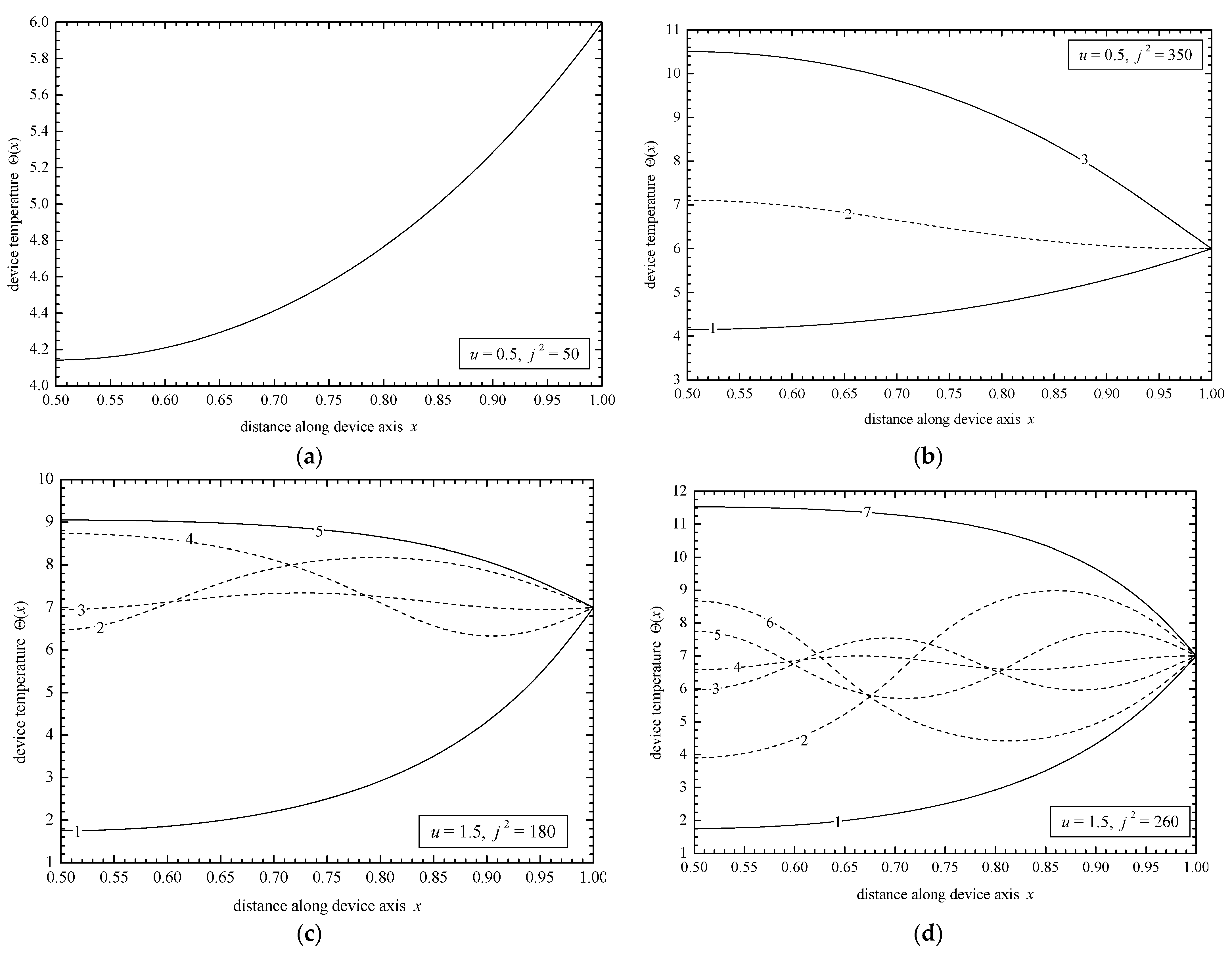
Interestingly, when the conduction term and the associated conduction–convection parameter u is taken into consideration, a far more complicated solution structure and multiplicity pattern emerges, as shown in Figure 4, where the edge temperature is plotted against . For lower values of the conduction–convection parameter , the three uniform solutions of Equation (24) are recovered (Figure 4a). As u increases, the number of solutions increases as well. Five solutions exist for in Figure 4b, seven solutions for in Figure 4c, and eleven for in Figure 4d. The corresponding temperature profiles are shown in Figure 5a–d. In every case, the solution structure consists of the three uniform solutions: one stable “cold”, one stable “hot”, and one unstable at an intermediate temperature. Additional unstable solutions emerge in the form of standing waves as u gradually increases. It is worth pointing out that the solution obtained by imposing the boundary conditions in Equation (20) have two salient features. The first one is that as long as the nonuniform solutions are unstable, only the uniform ones are physically encountered, with the “cold” one being far more preferable from the operating point of view, since it results in the reduced thermal stresses and thermal loading (reduced fracture probability) of the device, as already explained in the previous paragraph. The second feature is a direct consequence of the first one, since the stable temperature profiles may be obtained from the solution of the much simpler algebraic problem in Equation (24) instead of solving the complete boundary value problem of Equation (17). Hence, the results concerning the bistability and the magnitude of the “hot” temperature previously obtained from the lumped (zero-dimensional) model are verified from the one-dimensional model as well. The hypothesis put forward of the induced thermal shock during the changeover from the “cold” to the “hot” state is further supported from the similar behavior encountered in other bistable systems, as in, for example, superconductors, when, for instance, a current lead feeding a superconductor magnet made from a high temperature superconductor switches from the superconducting (“cold”) state to the normal one (“hot”), say because of a loss of coolant flow accident, and then the temperature level could be in excess of 3000 K (see Krikkis [44] for a numerical calculation and Dresner [49] in paragraphs 10.3 to 10.8 for an analytical one under certain simplifying assumptions). The reason for such a similarity is the form of the electric resistivity, where, within a short temperature range, the resistivity changes by several orders of magnitude. The same bistability and hysteresis loops occur in boiling systems through the nonlinear and nonmonotonic boiling curve describing the three boiling modes, the stable nucleate and film, and the unstable transition one. When the wall temperature exceeds the critical heat flux, the system experiences a jump-like behavior, as shown in Figure 3, from the nucleate (“cold”) regime to the film (“hot”) regime and vice versa. The latter entails a significantly higher temperature (Zhukov and Barelko [50], Krikkis [51]). This nonlinear behavior is well understood and documented both theoretically and experimentally.
3.2. Problem P2
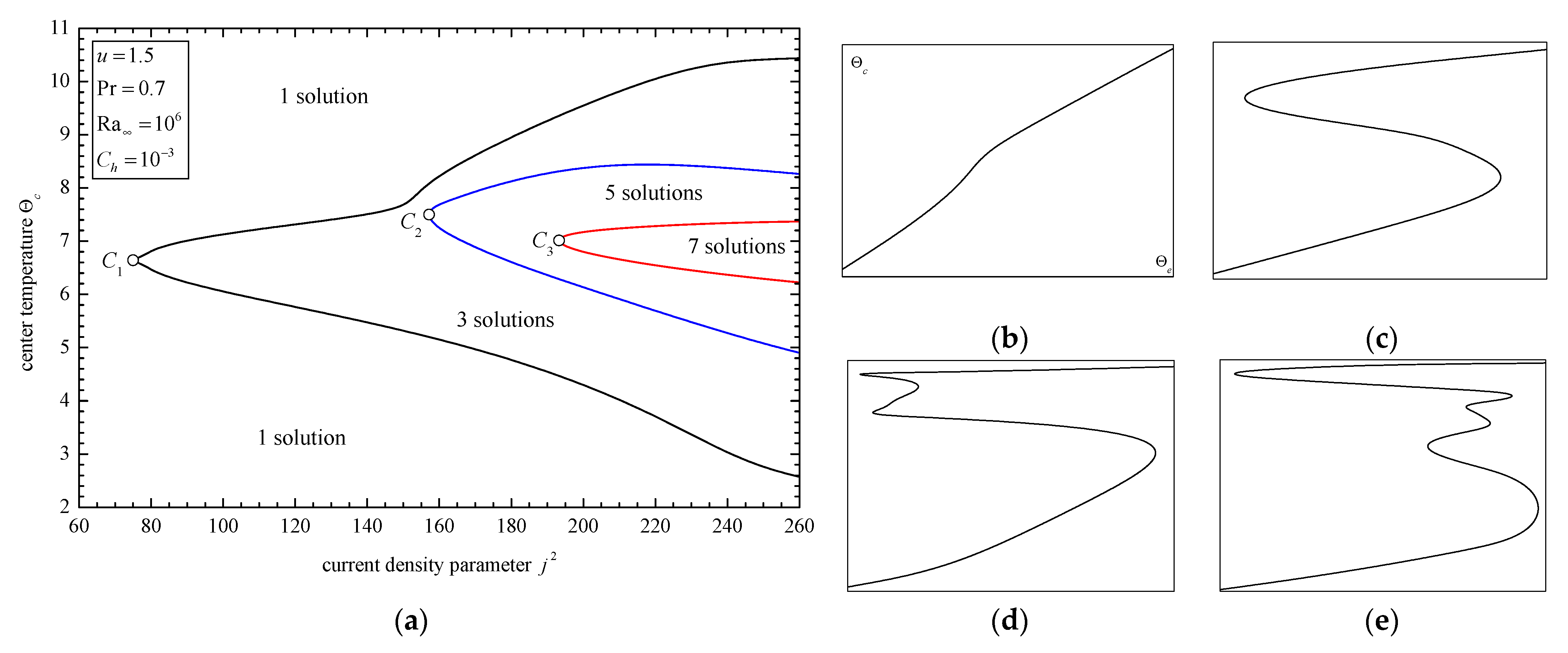
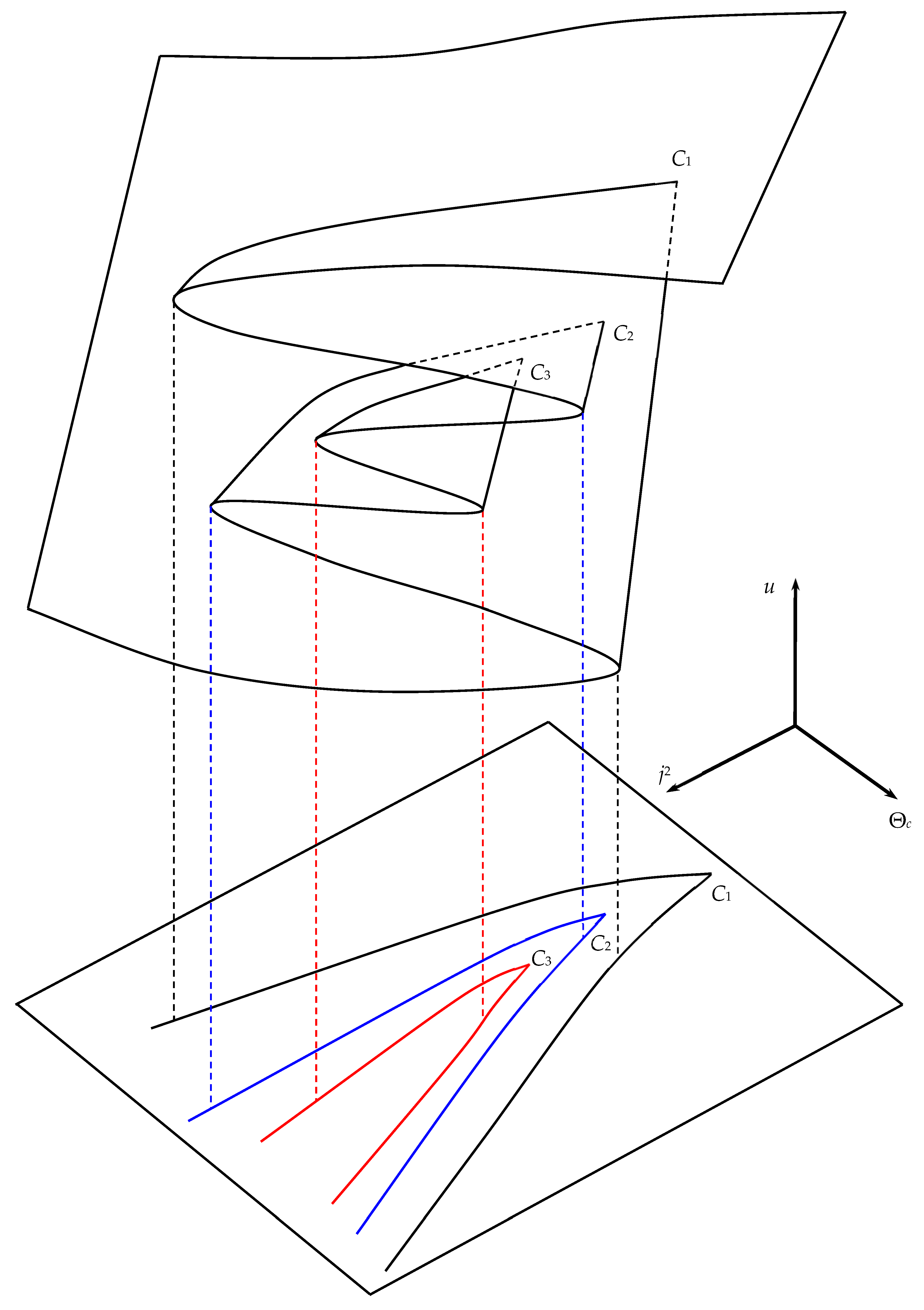
For the case where the edge temperature is fixed, the bifurcation analysis reveals a rich and interesting pattern, as shown in Figure 6. Selecting the center temperature as the bifurcation parameter, the projection of the limit points on the plane forms a pattern of nested cusp points in Figure 6a, where the regions with unique, three, five, and seven (and so on) solutions are designated accordingly. For a better understanding of the complexity of the solution structure and the clarity of the exposition, a geometrical perspective of the nested cusps is depicted in Figure 7. Again, the CCP has a profound effect on the solution structure, since the number of steady states calculated depends on its magnitude. Indeed, starting from and a unique solution in Figure 6b, three solutions emerge for in Figure 6c, five for in Figure 6d, and seven in Figure 6e for . The temperature profiles for problem P2 are symmetrical with respect to the center of the device. For the unique solution calculated in Figure 8a, the center is maintained at a lower temperature, while the temperature increases towards the edge . When the CCP increases and three solutions are present, as in Figure 8b, for the same edge temperature , two stable solutions exist: one “cold” and one “hot” . In contrast to the “cold” solution described earlier, the peak temperature for the “hot” one now appears around the center and gradually decreases to . As CCP further increases, more solutions emerge: five in Figure 8c for and seven in Figure 8d when . The stable ones remain as the “cold” and “hot” set described earlier, whereas the ones appearing as standing waves are unstable. In other words, the bistability is retained as the CCP increases and several additional solutions emerge. Furthermore, as u increases, a temperature plateau around the center is formed and the temperature gradient along the device, although it cannot be entirely eliminated as was the case in problem P1, is definitely reduced. It is worth pointing out that a multiplicity structure consisting of nested cusps is not a unique feature of this particular electrothermal problem. Aris [52] was the first to publish imbedded cusps in the study of first-order reactions in a spherical pellet. The same solution structure emerged in the analysis of another chemical reacting system, namely, an isothermal Langmuir–Hinshelwood reaction in a cylindrical or spherical pellet (Witmer et al. [53]). Another example of similar multiplicity behavior is encountered when the three boiling modes (nucleate, transition, and film) are excited by a uniform heat-generating source along a non-isothermal extended surface immersed in a boiling liquid (Krikkis [51]).
3.3. Voltage Control Problems P1 and P2
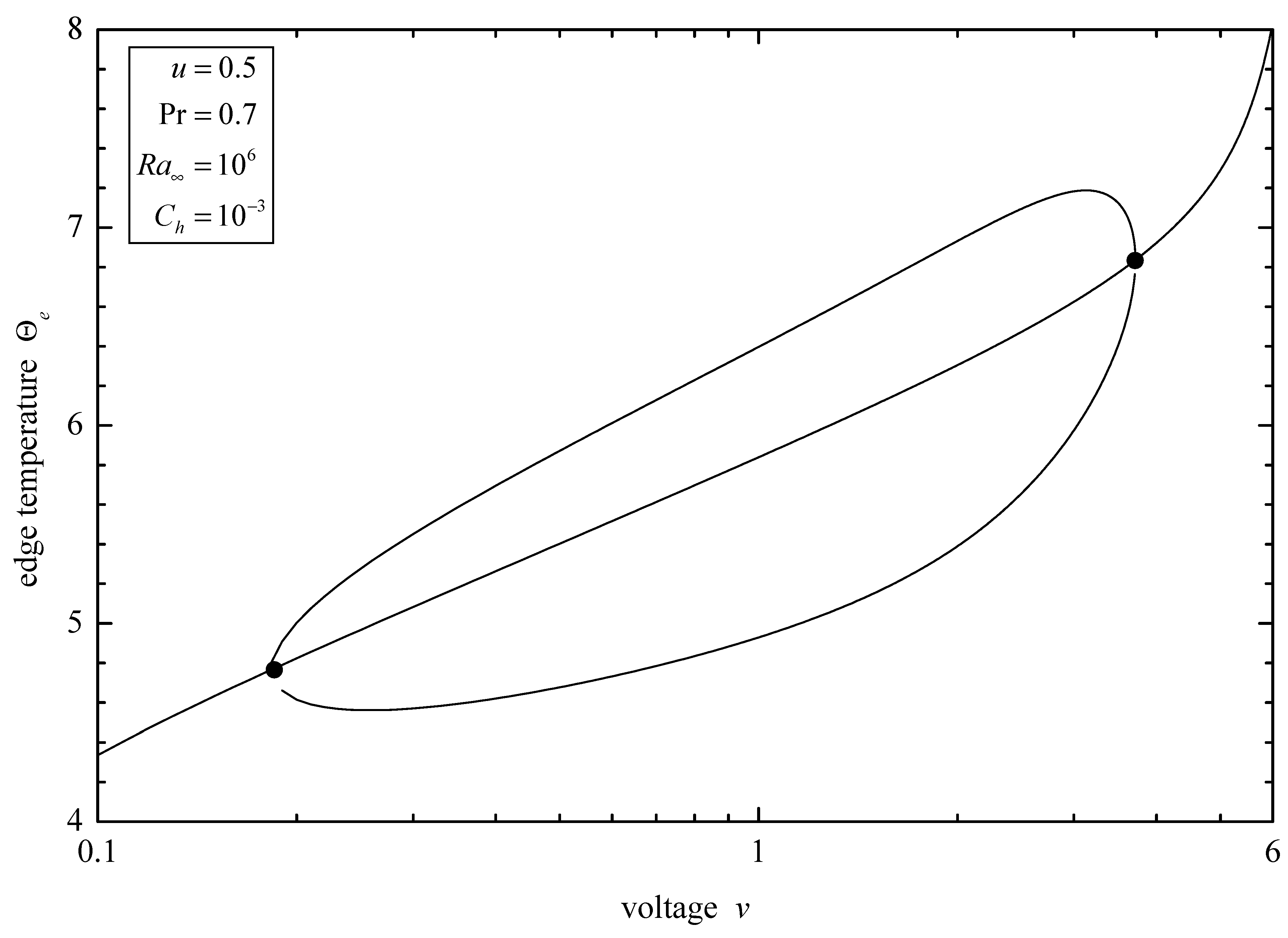
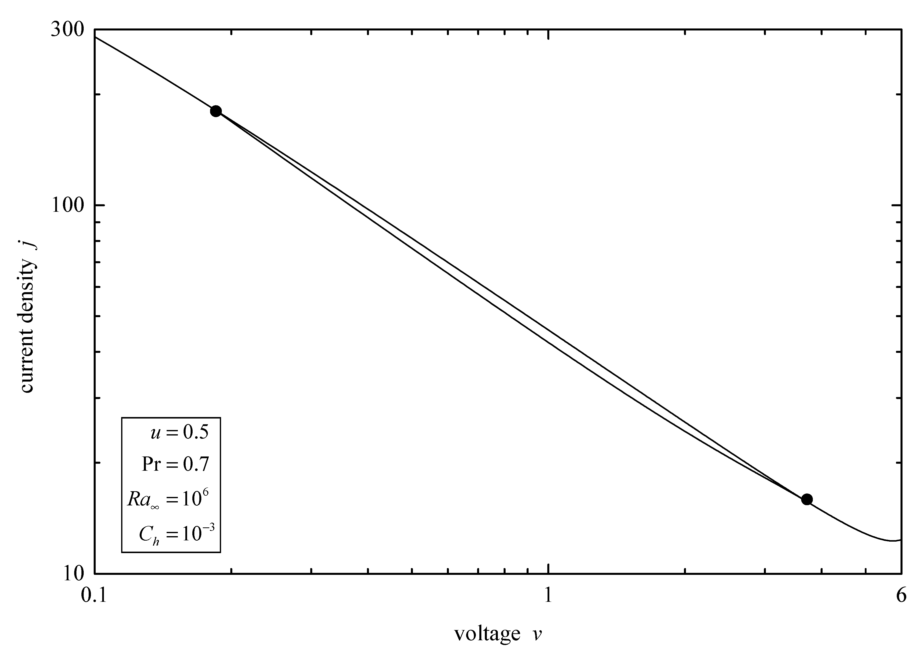
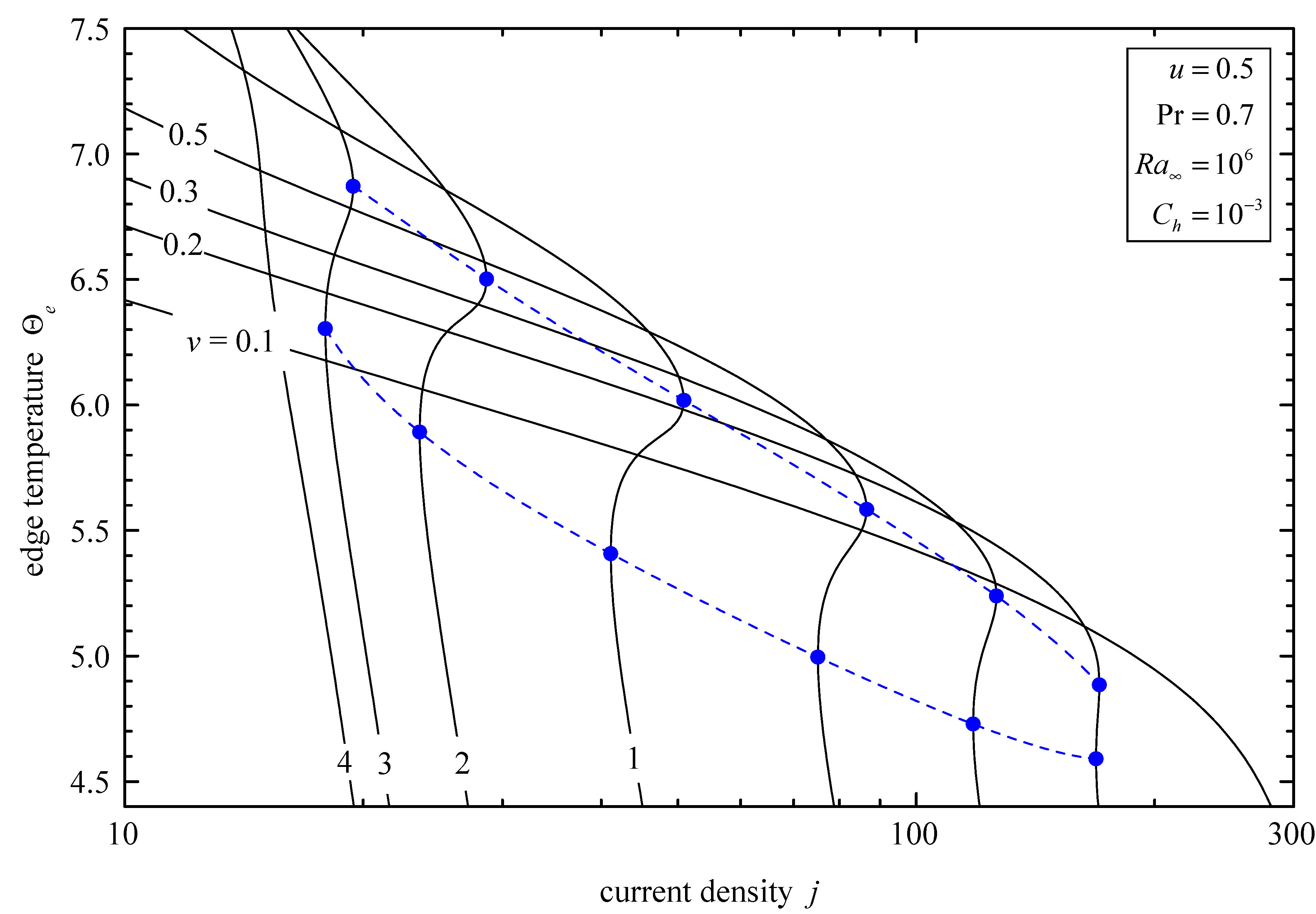
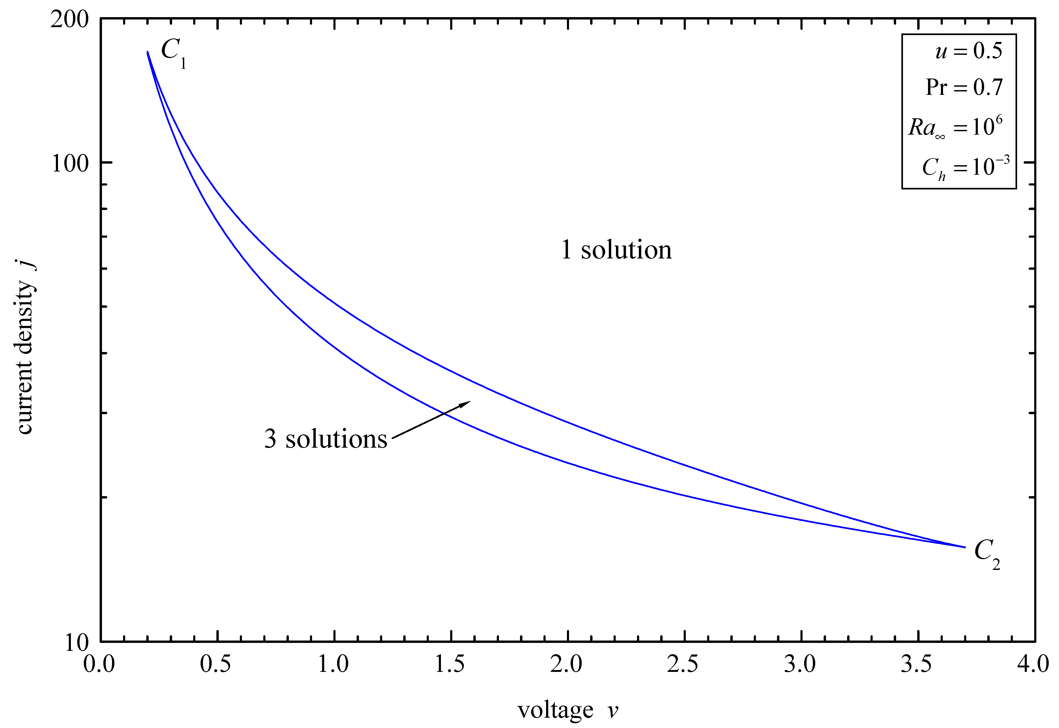
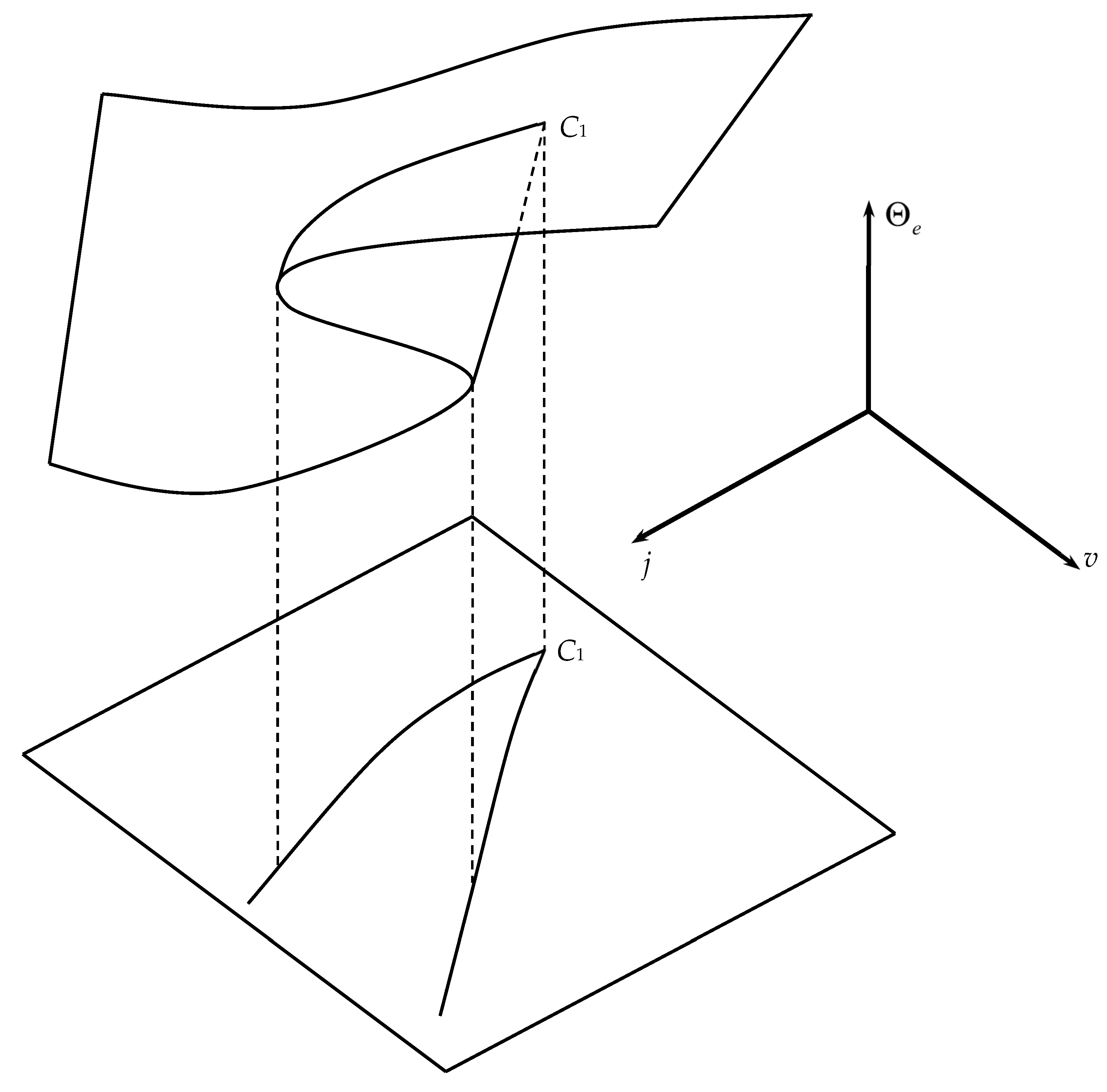
For the range of parameters considered when the voltage is the controlling parameter, the nonlocal problem in Equation (18) admits up to three solutions, as shown from the multiplicity pattern on the plane in Figure 9 and from current–voltage characteristic in Figure 10 for problem P1. Two singular points exist and the temperature remains bounded for both problems P1 and P2. Clearly, this a key feature of PTC resistivity. In comparison, the multiplicity pattern for an NTC resistivity characteristic is simpler as it is restricted to a single limit point, but it is associated with an unbounded temperature (thermal runaway) once the voltage exceeds this limit point, leading to the so-called flash sintering phenomenon. Moreover, from a practical point of view, Figure 10 demonstrates the device potential for use as a current limiter, since the current density decreases with the applied voltage both in the regions with a unique solution and within the multiplicity region. When the heat transfer from the device edges (problem P2) is taken into account, again, up to three solutions exist, but the solution structure is qualitatively different. A bifurcation diagram on the plane with the applied voltage v as a parameter is depicted in Figure 11. Along a line of constant voltage, the edge temperature shows only a weak dependence on the applied current, and in effect, the temperature is mostly affected by the voltage. Projecting the limit points of Figure 11 onto the , plane we obtain the multiplicity region of the voltage–current characteristic shown in Figure 12. For this case, the multiplicity domain is confined between two cusp points, C1 and C2, respectively. For a better understanding of the solution structure, a geometrical representation of the associated cusp point is shown in Figure 13.
4. Conclusions and Future Work
An electrothermal model for a barium titanate-based PTC thermistor has been set up, featuring a nonlinear heat rejection mechanism consisting of natural convection combined with radiation through the device’s lateral surface. A smooth and strongly temperature-dependent electric conductivity function based on experimental data has been adopted. The temperature field has been resolved for both cases, where either the current or the voltage (nonlocal problem) is the controlling parameter. With the aid of an efficient continuation algorithm, multiple steady-state solutions that do not depend on the external circuit have been identified as a result of the inherent nonlinearities. Important findings are the profound effect of the conduction–convection parameter and of the boundary conditions on the multiplicity structure.
For the current control case, regardless of the type of boundary conditions imposed, the number of multiple steady states depends on the magnitude of the conduction–convection parameter, as, for instance, up to eleven solutions have been calculated when the edges of the device are insulated (problem P1) and up to seven when the edge temperature is being fixed (problem P2). The stability analysis reveals that for problem P1, only the uniform solutions are stable, namely, one “cold” and one “hot”. A key feature of this bistability is that the “cold” solution remains constant and close to the ambient temperature for a wide range of applied currents, but on the other hand, the “hot” steady state is proportional to the input power and the temperature is substantially higher. Therefore, a change in the operating point from the “cold” to the “hot” state closely resembles thermal shock, and could perhaps be a reason for the mechanical failure (delamination fracture) of PTC thermistors. Therefore, the control and effective reduction of the heat transmitted through the edges results in the reduced thermal loading of the device both in the steady-state operation and during transients, since the temperature gradient across the device vanishes. On the other hand, when the voltage is controlled, the multiple solutions are reduced to three, while the maximum temperature appears lower compared with the current controlled case.
As for future work, it would be interesting to extend the analysis to 2D/3D geometries and include alternating voltage and current as the controlling parameters. Another research direction could be the potential multiplicity features of ceramic devices with more complicated electrical resistivity functions resembling a combination of positive–negative temperature coefficients, as, for instance, those reported by Takeda et al. [38] and Fang et al. [54]. This particular form of the resistivity admits self-sustained oscillations (Hopf bifurcation), introducing a challenging dynamic behavior, as shown by Elmer [55].
Funding
This research received no external funding.
Institutional Review Board Statement
Not applicable.
Informed Consent Statement
Not applicable.
Conflicts of Interest
The author declares no conflict of interest.
Nomenclature
| A | Cross-sectional area | (m2) |
| C | specific heat capacity | (J/(kgK)) |
| D | device diameter | (m) |
| E | electric field intensity | (V/m) |
| f | function of Prandtl number in Equation (7) | (-) |
| g | acceleration due to gravity | (-) |
| convective heat transfer coefficient | (W/(m2K)) | |
| radiative heat transfer coefficient | (W/(m2K)) | |
| j | current density parameter | (-) |
| J | current density | (A/m2) |
| k | thermal conductivity | (W/(mK)) |
| L | device length | (m) |
| Nu | Nusselt number, Equation (7) | (-) |
| P | perimetry | (m) |
| Pr | Prandtl number, Equation (7) | (-) |
| Ra | Rayleigh number, Equation (8) | (-) |
| t | time | (s) |
| T | temperature | (K) |
| u | conduction–convection parameter | (-) |
| v | dimensionless voltage drop | (-) |
| V | voltage drop | (V) |
| x | dimensionless distance | (-) |
| X | longitudinal distance along device | (m) |
Greek Symbols
| α | thermal diffusivity | (m2/s) |
| β | thermal expansivity | (K−1) |
| γ | material density | (kg/m3) |
| ε | emissivity | (-) |
| Θ | dimensionless temperature | (-) |
| λ | eigenvalue | (-) |
| ν | kinematic viscosity | (m2/s) |
| ρ | reduced electric resistivity | (-) |
| electric resistivity | (Ω m) | |
| σ | Stefan–Boltzmann constant | (Wm−2K−4) |
| τ | dimensionless time | (-) |
| electric potential | (V) |
Subscripts
| b | |
| c | |
| e | |
| ref | reference value |
| s | steady state |
| ∞ | ambient environment |
Superscripts
| derivative with respect to x |
Abbreviations
| CCP | conduction–convection parameter |
| NTC | negative temperature coefficient |
| PTC | positive temperature coefficient |
References
- Glaggett, T.G.; Worrall, R.W.; Lipták, B.G.; Silva Girão, P.M.B. Thermistors. In Instrument Engineers’ Handbook, Process Measurement and Analysis, 4th ed.; Lipták, B.G., Ed.; CRC Press: Boca Raton, FL, USA, 2003; Volume 1, pp. 666–672. [Google Scholar]
- Fraden, J. Handbook of Modern Sensors. Physics, Designs and Applications, 3rd ed.; AIP Press: New York, NY, USA, 2004; pp. 477–481. [Google Scholar]
- Sapoff, M. Thermistor Thermometers. In The Measurement, Instrumentation and Sensors Handbook; Webster, J.G., Ed.; CRC Press: Boca Raton, FL, USA; IEEE Press: Piscataway, NJ, USA, 1999. [Google Scholar]
- Naik, A.U.; Mallick, P.; Sahu, M.K.; Biswal, L.; Satpathy, S.K.; Behera, B. Investigation on Temperature-Dependent Electrical Transport Behavior of Cobalt Ferrite (CoFe2O4) for Thermistor Applications. ECS J. Solid State Sci. Technol. 2023, 12, 053007. [Google Scholar] [CrossRef]
- Mallick, P.; Satpathy, S.K.; Behera, B. Study of Structural, Dielectric, Electrical, and Magnetic Properties of Samarium-Doped Double Perovskite Material for Thermistor Applications. Braz. J. Phys. 2022, 52, 187. [Google Scholar] [CrossRef]
- Dewitte, C.; Elst, R.; Delannay, F. On the mechanism of delamination fracture of BaTiO3-based PTC thermistors. J. Eur. Ceram. Soc. 1994, 14, 481–492. [Google Scholar] [CrossRef]
- Supancic, P. Mechanical stability of BaTiO3-based PTC thermistors components: Experimental investigation and theoretical modeling. J. Eur. Ceram. Soc. 2000, 20, 2009–2024. [Google Scholar] [CrossRef]
- Danzer, R.; Kaufmanna, B.; Supancic, P. Failure of high power varistor ceramic components. J. Eur. Ceram. Soc. 2020, 40, 3766–3770. [Google Scholar] [CrossRef]
- Diesselhorst, H. Uber das Probleme das Electrisch Erwärmter Leiter. Ann. Phys. 1900, 1, 312–325. [Google Scholar] [CrossRef]
- Cimatti, G. Remark on existence and uniqueness for the thermistor problem under mixed boundary conditions. Quart. Appl. Math. 1989, 47, 117–121. [Google Scholar] [CrossRef]
- Cimatti, G. A bound for temperature in thermistor problem. IMA J. Appl. Math. 1988, 40, 15–22. [Google Scholar] [CrossRef]
- Cimatti, G.; Prodi, G. Existence results for a nonlinear elliptic system modeling a temperature dependent electrical resistor. Ann. Mat. Pure Appl. 1988, 152, 227–236. [Google Scholar] [CrossRef]
- Xie, H.; Allegretto, W. Ca (Ω) solutions of a class of nonlinear degenerate elliptic systems arising in the thermistor problem. SIAM J. Math. Anal. 1991, 22, 1491–1499. [Google Scholar] [CrossRef]
- Antontsev, S.N.; Chipot, M. The Thermistor Problem: Existence, smoothness, uniqueness, blowup. SIAM J. Math. Anal. 1994, 25, 1128–1156. [Google Scholar] [CrossRef]
- Bahadir, A.R. Steady state solution of the PTC thermistor using a quadratic spline finite element method. Math. Methods Eng. 2002, 8, 101–109. [Google Scholar] [CrossRef]
- Bahadir, A.R. Application of cubic B-spine finite element technique to the thermistor problem. Appl. Math. Comput. 2004, 149, 379–387. [Google Scholar]
- Çatal, S. Numerical solution of the thermistor problem. Appl. Math. Comput. 2004, 152, 743–757. [Google Scholar] [CrossRef]
- Kutluay, S.; Wood, A.S.; Esen, A. A heat balance integral solution of the thermistor with a modified electrical conductivity. Appl. Math. Model. 2006, 30, 386–394. [Google Scholar] [CrossRef]
- Ammi, M.R.S.; Torres, D.F.M. Numerical analysis of a nonlocal parabolic problem resulting from thermistor problem. Math. Comput. Simul. 2008, 77, 291–300. [Google Scholar] [CrossRef]
- Golosnoy, I.O.; Sykulski, J.K. Numerical modeling of non-linear coupled thermo-electric problems. A comparative study. Int. J. Comput. Math. Electr. Electron. Eng. 2009, 28, 639–655. [Google Scholar] [CrossRef]
- Bistability, E.G.K. autowaves and dissipative structures in semiconductor fibers with anomalous resistivity properties. Philos. Mag. 2012, 92, 1300–1316. [Google Scholar]
- Hewitt, I.J.; Lacey, A.A.; Todd, R.I. A mathematical model for flash sintering. Math. Model. Nat. Phenom. 2015, 10, 77–89. [Google Scholar] [CrossRef]
- Raj, R. Joule heating during flash-sintering. J. Eur. Ceram. Soc. 2012, 32, 2293–2301. [Google Scholar] [CrossRef]
- Todd, R.I.; Zapata-Solvas, E.; Bonilla, R.S.; Sneddon, T.; Wilshaw, P.R. Electrical characteristics of flash sintering: Thermal runaway of Joule heating. J. Eur. Ceram. Soc. 2015, 35, 1865–1877. [Google Scholar] [CrossRef]
- da Silva, J.G.P.; Al-Qureshi, H.A.; Keil, F.; Janssen, R. A dynamic bifurcation criterion for thermal runaway during the flash sintering of ceramics. J. Eur. Ceram. Soc. 2016, 36, 1261–1267. [Google Scholar] [CrossRef]
- Fowler, A.C.; Frigaard, I.; Howison, S.D. Temperature surges in current-limiting circuit devices. SIAM J. Appl. Math. 1992, 52, 998–1011. [Google Scholar] [CrossRef]
- Howison, S.D.; Rodrigues, J.F.; Shilor, M. Stationary solutions to the thermistor problem. J. Math. Anal. And. Appl. 1993, 174, 573–588. [Google Scholar] [CrossRef]
- Zhou, S.; Westbrook, D.R. Numerical solutions of the thermistor equations. J. Comput. Appl. Math. 1997, 79, 101–118. [Google Scholar] [CrossRef]
- Cimatti, G. Remark on the number of solutions in the thermistor problem. Le Math. 2011, 66, 49–60. [Google Scholar]
- Metaxas, A.C. Foundations of Electroheat. A Unified Approach; John Wiley & Sons: New York, NY, USA, 1996. [Google Scholar]
- Lupi, S. Foundamentals of Electroheat. Electrical Technologies for Process Heating; Springer: Cham, Switzerland, 2017. [Google Scholar]
- Aliferov, A.; Lupi, S.; Forzan, M. Induction and Direct Resistance Heating. Theory and Numerical Modeling; Springer: Cham, Switzerland, 2015. [Google Scholar]
- Touzani, R.; Rappaz, J. Mathematical Models for Eddy Currents and Magnetostatics; Springer: Cham, Switzerland, 2014. [Google Scholar]
- Brzozowski, E.; Castro, M.S. Conduction mechanism of barium titanate ceramics. Ceram. Int. 2000, 26, 265–269. [Google Scholar] [CrossRef]
- Wang, X.; Chan, H.L.W.; Choy, C.L. Semiconducting barium titanate ceramics prepared by using yttrium hexaboride as sintering aid. Mater. Sci. Eng. B 2003, 100, 286–291. [Google Scholar] [CrossRef]
- Wang, X.; Pang, H.L.W.C.G.K.H.; Choy, C.L. Positive temperature coefficient of resistivity effect in niobium doped barium titanate ceramics obtained at low sintering temperature. J. Eur. Ceram. Soc. 2004, 24, 1227–1231. [Google Scholar] [CrossRef]
- Luo, Y.; Liu, X.; Li, X.; Liu, G. PTCR effect in BaBiO3-doped BaTiO3 ceramics. Solid State Ionics 2006, 177, 1543–1546. [Google Scholar] [CrossRef]
- Takeda, H.; Harinaka, H.; Shiosaki, T.; Zubair, M.A.; Leach, C.; Freer, R.; Hoshina, T.; Tsurumi, T. Fabrication and positive temperature coefficient of resistivity properties of semiconducting ceramics based on the BaTiO3-(Bi1/2K1/2)TiO3 system. J. Eur. Ceram. Soc. 2010, 30, 555–559. [Google Scholar] [CrossRef]
- Rowlands, W.; Vaidhyanathan, B. Additive manufacturing of barium titanate based ceramic heaters with positive temperature coefficient (PTCR). J. Eur. Ceram. Soc. 2019, 39, 3475–3483. [Google Scholar] [CrossRef]
- Churchill, S.W.; Chu, H.H.S. Correlating equations for laminar and turbulent free convection from a horizontal cylinder. Int. J. Heat. Mass Transf. 1975, 18, 1049–1053. [Google Scholar] [CrossRef]
- Faghri, M.; Sparrow, E.M. Forced convection in a horizontal pipe subjected to nonlinear external natural convection and to external radiation. Int. J. Heat. Mass Transf. 1986, 23, 861–872. [Google Scholar] [CrossRef]
- Krikkis, R.N. Laminar conjugate forced convection over a flat plate. Multiplicities and stability, Int. J. Therm. Sci. 2017, 111, 204–214. [Google Scholar] [CrossRef]
- Krikkis, R.N. On the Thermal Dynamics of Metallic and Superconducting Wires. Bifurcations, Quench, the Destruction of Bistability and Temperature Blowup. J 2021, 4, 803–823. [Google Scholar] [CrossRef]
- Krikkis, R.N. Analysis of High-Temperature Superconducting Current Leads: Multiple Solutions, Thermal Runaway, and Protection. J 2023, 6, 302–317. [Google Scholar] [CrossRef]
- Hairer, E.; Nørsett, S.P.; Wanner, G. Solving Ordinary Differential Equations I. Nonstiff Problems; Springer-Verlag: New York, NY, USA, 1987. [Google Scholar]
- Ascher, U.M.; Mattheij, R.M.M.; Russel, R.D. Numerical Solution of Boundary Value Problems for Ordinary Differential Equations, 2nd ed.; SIAM: Philadelphia, PA, USA, 1995. [Google Scholar]
- Seydel, R. Practical Bifurcation and Stability Analysis, 3rd ed.; Springer: New York, NY, USA, 2009. [Google Scholar]
- Witmer, G.; Balakotaih, V.; Luss, D. Finding singular points of two-point boundary value problems. J. Comput. Phys. 1986, 65, 244–250. [Google Scholar] [CrossRef]
- Dresner, L. Stability of Superconductors; Springer+Bussiness Media: New York, NY, USA, 1995. [Google Scholar]
- Zhukov, S.A.; Barelko, V.V. Nonuniform steady states of the boiling process in the transition region between the nucleate and film regimes. Int. J. Heat. Mass Transf. 1983, 26, 1121–1130. [Google Scholar] [CrossRef]
- Krikkis, R. On the multiple solutions of boiling fins with heat generation. Int. J. Heat. Mass Transf. 2015, 80, 236–242. [Google Scholar] [CrossRef]
- Aris, R. Chemical reactors and some bifurcation phenomena. Ann. N. Y. Acad. Sci. 1979, 316, 314–331. [Google Scholar] [CrossRef]
- Witmer, G.; Balakotaih, V.; Luss, D. Multiplicity features of distributed systems—I. Langmuir-Hinshelwood reaction in a porous catalyst. Chem. Eng. Sci. 1986, 41, 179–186. [Google Scholar] [CrossRef]
- Fang, C.; Zhou, D.-X.; Gong, S.-P. Voltage effects in PTCR ceramics: Calculation by the method of tilted energy bands. Phys. B 2010, 65, 852–856. [Google Scholar] [CrossRef]
- Elmer, F.J. Limit cycles of the ballast resistor caused by intrinsic instabilities. Z. Phys. B Condens. Matter 1992, 87, 377–386. [Google Scholar] [CrossRef]
Figure 1.
Conductor geometry and energy balance.

Figure 2.
Uniform solutions and energy balance on the device. (a) Heat dissipation by primarily natural convection and (b) by combined natural convection and radiation.
Figure 2.
Uniform solutions and energy balance on the device. (a) Heat dissipation by primarily natural convection and (b) by combined natural convection and radiation.

Figure 3.
Hysteresis loop. Temperature versus current density for uniform states.

Figure 4.
Multiplicity pattern for current control problem P1. (a) Three uniform solutions, . (b) Five solutions, . (c) Seven solutions, . (d) Eleven solutions, . Solid line: stable, dashed line: unstable.
Figure 4.
Multiplicity pattern for current control problem P1. (a) Three uniform solutions, . (b) Five solutions, . (c) Seven solutions, . (d) Eleven solutions, . Solid line: stable, dashed line: unstable.

Figure 5.
Solution structure for current control problem P1, corresponding to multiplicity pattern in Figure 4. (a) Three uniform solutions, . (b) Five solutions, . (c) Seven solutions, . (d) Eleven solutions, . Solid line: stable, dashed line: unstable.
Figure 5.
Solution structure for current control problem P1, corresponding to multiplicity pattern in Figure 4. (a) Three uniform solutions, . (b) Five solutions, . (c) Seven solutions, . (d) Eleven solutions, . Solid line: stable, dashed line: unstable.


Figure 6.
Current control problem P2. (a) Projection of the singular points on the plane. (b) One solution, , (c) three solutions, , (d) five solutions, , and (e) seven solutions, .
Figure 6.
Current control problem P2. (a) Projection of the singular points on the plane. (b) One solution, , (c) three solutions, , (d) five solutions, , and (e) seven solutions, .

Figure 7.
Current control problem P2. Geometrical perspective of nested cusps and projection of the limit points on the plane.
Figure 7.
Current control problem P2. Geometrical perspective of nested cusps and projection of the limit points on the plane.

Figure 8.
Solution structure for current control problem P2, corresponding to multiplicity pattern in Figure 4. (a) Three uniform solutions, . (b) Five solutions, . (c) Seven solutions, . (d) Eleven solutions, . Solid line: stable, dashed line: unstable.
Figure 8.
Solution structure for current control problem P2, corresponding to multiplicity pattern in Figure 4. (a) Three uniform solutions, . (b) Five solutions, . (c) Seven solutions, . (d) Eleven solutions, . Solid line: stable, dashed line: unstable.

Figure 9.
Voltage control problem P1. Multiple solutions on the plane.

Figure 10.
Voltage control problem P1. Multiple solutions on the plane.

Figure 11.
Voltage control problem P2. Multiple solution the plane.

Figure 12.
Voltage control problem P2. Projection of the limit points on the plane.

Figure 13.
Voltage control problem P2. Geometrical perspective of a single cusp point and projection of the limit points on the plane.
Figure 13.
Voltage control problem P2. Geometrical perspective of a single cusp point and projection of the limit points on the plane.

Disclaimer/Publisher’s Note: The statements, opinions and data contained in all publications are solely those of the individual author(s) and contributor(s) and not of MDPI and/or the editor(s). MDPI and/or the editor(s) disclaim responsibility for any injury to people or property resulting from any ideas, methods, instructions or products referred to in the content. |
© 2023 by the author. Licensee MDPI, Basel, Switzerland. This article is an open access article distributed under the terms and conditions of the Creative Commons Attribution (CC BY) license (https://creativecommons.org/licenses/by/4.0/).
Share and Cite
MDPI and ACS Style
Krikkis, R.N. Multiplicity Analysis of a Thermistor Problem—A Possible Explanation of Delamination Fracture. J 2023, 6, 517-535. https://doi.org/10.3390/j6030034
AMA Style
Krikkis RN. Multiplicity Analysis of a Thermistor Problem—A Possible Explanation of Delamination Fracture. J. 2023; 6(3):517-535. https://doi.org/10.3390/j6030034
Chicago/Turabian StyleKrikkis, Rizos N. 2023. "Multiplicity Analysis of a Thermistor Problem—A Possible Explanation of Delamination Fracture" J 6, no. 3: 517-535. https://doi.org/10.3390/j6030034