Efficient Color Correction Using Normalized Singular Value for Duststorm Image Enhancement

Abstract

A duststorm image has a reddish or yellowish color cast. Though a duststorm image and a hazy image are obtained using the same process, a hazy image has no color distortion as it has not been disturbed by particles, but a duststorm image has color distortion owing to an imbalance in the color channel, which is disturbed by sand particles. As a result, a duststorm image has a degraded color channel, which is rare in certain channels. Therefore, a color balance step is needed to enhance a duststorm image naturally. This study goes through two steps to improve a duststorm image. The first is a color balance step using singular value decomposition (SVD). The singular value shows the image’s diversity features such as contrast. A duststorm image has a distorted color channel and it has a different singular value on each color channel. In a low-contrast image, the singular value is low and vice versa. Therefore, if using the channel’s singular value, the color channels can be balanced. Because the color balanced image has a similar feature to the haze image, a dehazing step is needed to improve the balanced image. In general, the dark channel prior (DCP) is frequently applied in the dehazing step. However, the existing DCP method has a halo effect similar to an over-enhanced image due to a dark channel and a patch image. According to this point, this study proposes to adjustable DCP (ADCP). In the experiment results, the proposed method was superior to state-of-the-art methods both subjectively and objectively.

1. Introduction

The haze image seems dimmed due to haze particles, but all color channels have the fit in balance. In the process of improving a haze image, a dehazing step is needed. A duststorm image and a hazy image have a similar category in the obtaining process; thus, a dehazing step is needed to enhance a duststorm image and a haze image. Although the duststorm image has a similar feature with the haze image, this has distortion in some color channels (green and blue channels), and this makes the color cast image; reddish or yellowish. Therefore, a color balance step is needed to enhance a degraded duststorm image. If not, a new artifact color distortion can appear in the enhanced image.

There have been many studies on the dehazing method. He et al. [1] proposed the dark channel prior (DCP) to enhance a hazy image. The DCP estimates the dark region in an image [1]. Though the DCP [1] method estimates the dark region of a color channel, if the image has the sky region, the DCP image is not dark but bright. Due to this, the enhanced image has the halo effect such as a color shift. Meng et al. tried to enhance a hazy image using a boundary constraint on the transmission map [2]. This method has a strong point in the sky region of transmission map. In general, the transmission map by DCP has the halo effect in the sky region. However, the transmission map in Meng et al.’s method has a natural transmission map, and the enhanced image seems natural [2]. However, the thick haze region is not enhanced well [2]. Zhu et al. proposed a dehazing method using a color attenuation prior and a model that is the scene depth of a hazy image [3]. However, regardless of the scattering coefficient in the atmospheric scattering model, the halo effect appears [3].

The existing dehazing methods have a limitation in a duststorm image enhancement because of the color cast. Therefore, recently, there have been many works on duststorm image improvement to reduce the color distortion. Al-Ameen proposed a duststorm image enhancement method using a tuned fuzzy operation [4]. This method aims to enhance the image using tri thresholds and fuzzy operation on each color channel [4]. However, the weak point of this method is using the constant threshold, as it is not adaptive on various image. Naseeba et al. enhanced a duststorm image using tri modules [5]. This method enhances a duststorm image using the depth estimation module (DEM) with median filtering and gamma correction, a color analysis module (CAM) with gray assumption [6], and a visibility restoration module (VRM) [5]. Gao et al. insisted on the duststorm image enhancement method by reversing the blue channel prior (RBCP) [7]. This method improves the image by reversing the blue channel, which is often a rare component in a degraded duststorm image. Gao et al., using this property, enhanced a distorted duststorm image and corrected the color using the mean ratio of each color channel comparison with the red channel, which is mostly maintained in a distorted duststorm image. Gao et al.’s method is useful in duststorm image enhancement, but in a severely distorted duststorm image, the halo effect is shown still due to the rarity of the blue color channel. Shi et al. enhanced a duststorm image using the mean shift of color components [8]. This method uses the mean shift of color components to correct the distorted color. However, the new color shift can be seen in the enhanced image due to the mean shift. Cheng et al. improved a degraded duststorm image using color channel compensation and white balancing with robust automatic white balance (RAWB) [9] and enhanced the image using the guided image filtering [10,11]. This method is good at enhancing a duststorm image. However, due to just compensation on the blue channel, the halo effect can be seen. Shi et al. suggested a duststorm image enhancement method using normalized gamma correction and the mean shift of the color components [12]. This method is able to correct the color distortion. However, the artifact color distortion can be seen due to the mean shift of the color ingredients.

Recently, machine-learning-based dehazing algorithms have been studied. Wang et al. studied the dehazing method using atmospheric illumination prior [13]. This method works by estimating the atmospheric using the luminance channel, which has influence on a hazy image, and a hazy image is enhanced through the multi scale convolutional neural network (CNN) [13]. Zhang et al. worked to enhance a hazy image using multi scale CNN [14]. This method operates with three scales encoders and a fusion model [14]. Ren et al. tried to enhance a hazy image using multi-scale CNN [15]. This method consists of predicting the transmission map and refinement and goes through the multi-scale CNN (MSCNN) [15]. The machine-learning-based dehazing algorithms have a limitation in the correcting of the dataset, especially in a duststorm image.

There are many algorithms on the dehazing of an image. A duststorm image is similar to a dust or hazy image, if it is without the color distortion; a duststorm image has a yellowish or reddish color distortion. Therefore, a color correction step is needed to enhance a duststorm image. If not, the halo effect occurs in the enhanced image. To enhance a duststorm image naturally, this study proposes the two steps. The first is a color correction step. A duststorm image has a yellowish or reddish color cast caused by the degradation of the color channel such as the blue channel. To compensate for the color channel, this study uses the color channel’s singular value. The singular value of each color channel expresses the image’s feature. If the channel has low contrast, its singular value is low, and vice versa. If using this feature of the singular value, the relatively dark blue channel can be enhanced. A balanced duststorm image has a feature as with a hazy image. Therefore, to improve a balanced duststorm image, the dehazing algorithm is applied. In general, the existing dehazing algorithms use the DCP. However, the DCP has a weak point in the sky region. To complement this point, this study proposes the adjustable DCP. The improved image using the proposed method has no halo effect in comparison with the existing DCP. Additionally, when compared with other state-of-the-art methods, the experiment results of the proposed method are more subjectively and objectively compatible.

2. Background

A duststorm image is obtained through the atmosphere as with a hazy image. Many studies on enhancing a hazy image use the following mathematical Equation [16,17,18,19]:

$${\mathrm{I}}^c\left(\mathrm{x}\right)={\mathrm{J}}^c\left(\mathrm{x}\right)· t^c\left(x\right)+A^c·\left(1-t^c\left(x\right)\right)$$

(1)

where ${\mathrm{J}}^c\left(\mathrm{x}\right)$ is the scene radiance; $t^c\left(x\right)$ is the transmission map, which expresses the propagation path of the light; and $A^c$ is the back scatter light of the image; $\mathrm{c}\in \left\{\mathrm{r},\mathrm{g},\mathrm{b}\right\}$. As shown in Equation (1), a hazy image comprises the transmission map and back scatter light. A duststorm image is obtained by a similar process as the hazy image, as both images are obtained in the same medium. The equation of a duststorm image is also shown in Equation (1). The difference between a duststorm image and a hazy image is the presence of a color cast or not and attenuation. In general, a duststorm image has a reddish, yellowish color cast due to the sand particles with mineral. In addition, the duststorm image is attenuated by the dust particle, which has various sizes. The size of the dust is generally 1–63 microns [20,21], and the size of the sand particle is larger than 60 microns [20,21]. For this reason, the dust storm image looks dimmed and darkened; additionally, the dusty particles hinder the propagation of light. Therefore, this paper suggests, first, that the image’s color channel is improved to enhance a duststorm image. The second step is applying the dehazing step. The next sections introduce the color balance step and the dehazing step.

3. Proposed Method

3.1. Efficient Color Correction

A duststorm image has a reddish or yellowish color distortion owing to the imbalance of the color channel. It is a different feature to that of the haze image. Additionally, a duststorm image has various features due to the colorful sand particles and this hinders the propagation path of the light; a certain color channel such as green and blue is attenuated. When improving a duststorm image, if the distorted color channel is not corrected, the new artifact color distortion can be seen. Therefore, to enhance a duststorm image naturally, a color correction step is needed. In case of the white sand particles, a duststorm image seems to be a hazy image with color balance. However, if the duststorm particles have certain color, then the color channel degradation appears in the image. Therefore, to improve a duststorm image naturally, the image’s feature should be reflected. In general, a degraded duststorm image and its color channel have a different mean value. The mean value of the red channel is higher than that of green and blue. In a severely degraded duststorm image, the mean value of the blue channel is close to zero, and it also makes a degraded image when it is enhanced regardless of the color compensation. With this reason to correct the color channel, this study progresses with two steps. The first color correction step is based on the mean difference of each color channel. As mentioned above, the blue channel of a severely degraded image is rare. Considering this feature, if the mean difference of red and green is higher than that of blue, then the green and blue channels are corrected as follows:

$${\mathrm{I}}_m^{c^{\prime }}\left(\mathrm{x}\right)=\left(1-{\mathrm{I}}^{c^{\prime }}\left(x\right)\right)· G\left\{I\left(x\right)\right\}$$

(2)

$${\mathrm{I}}_{IB}^{c^{\prime }}\left(\mathrm{x}\right)={\mathrm{I}}^{c^{\prime }}\left(x\right)+I_m^{c^{\prime }}\left(x\right)· m\left(I_m^{c^{\prime }}\left(x\right)\right)$$

(3)

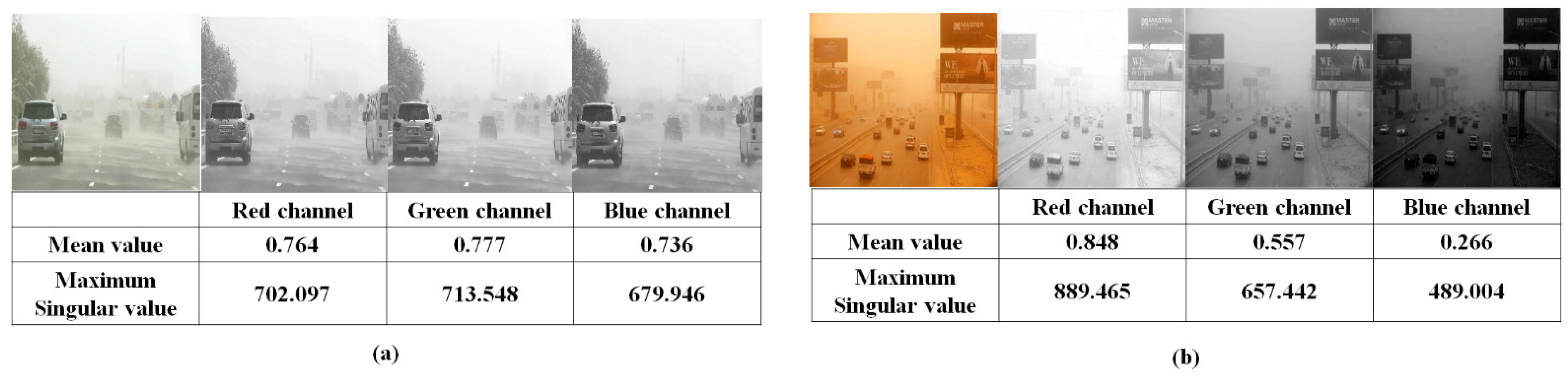
where ${\mathrm{I}}_m^{c^{\prime }}$(x) is the mask image on the severely degraded image $, \mathrm{G}\{·\}$ makes the gray scale image, $m(·)$ is the mean value of the color channel, ${\mathrm{I}}_{IB}^{c^{\prime }}\left(x\right)$ is the initial balanced image, ${\mathrm{c}}^{\prime }\in \left\{\mathrm{g},\mathrm{b}\right\},$ x is the location of pixel. Equations (2) and (3) are similar to the color balance method (CBM) [22], but the difference is that the CBM [22] used green channel to correct the color channel. However, to correct the color channel, using only the green channel is not sufficient. Meanwhile, the proposed color channel compensation method to correct the rare component uses the gray scale image to reflect the all channel’s feature. Although the rare channel is compensated, the color imbalance still exists in some severely degraded images. The degraded color channel has different features as, with a certain channel, it is attenuated in comparison with a non-degraded color channel. Additionally, it seems to have a dark and low contrast; in addition, its mean value is low and vice versa. In other words, an image’s contrast expresses the feature of the image. The singular values of the image have different features on the color channels, and these are variously used in the image processing area [23,24,25,26,27,28]. Li et al. denoised the image using SVD [28]. Tripathi et al. analyzed the image using SVD [26]. Halder et al. enhanced the image using SVD [27]. As the singular value is able to reflect an image’s feature, it is the efficient method to enhance the image. If an image is bright and its contrast is high, then its singular value is also high and vice versa. Figure 1 shows the relationship between an image’s singular value and its mean value on a color-degraded duststorm image and a not degraded duststorm image. As shown in Figure 1a, an undegraded duststorm image has a balanced color channel owing to its mean value and singular value being uniform, and there are no attenuated color channels. Meanwhile, the color degraded duststorm image has an imbalanced color channel such as Figure 1b. In particular, the blue channel is darker than other color channels, and its singular value and mean value are the lowest in the color channels, respectively. As known in Figure 1, the color balanced undegraded image has a uniform mean value and singular value on each color channel, but the degraded image does not have a uniform singular value in each color channel. If the color channel is not degraded, the singular value is high. However, if the color channel is degraded, the singular value is low. Therefore, this study uses the normalized singular value of each color channel to correct the degraded duststorm image. The singular value decomposition (SVD) procedure on each channel is described as follows:

$${\mathrm{I}}^c\left(x\right)=[{\mathrm{U}}^c, {\mathsf{\Sigma }}^c, {\mathrm{V}}^c]{ }^T$$

(4)

where ${\mathrm{I}}^c\left(x\right)$ is the input image; in this study, ${\mathrm{I}}^c\left(x\right)$ is using the ${\mathrm{I}}_{IB}^c\left(x\right)$ or ${\mathrm{I}}^c\left(x\right)$, selectively, following the mean difference; $x$ is the location of the pixel; ${\mathrm{U}}^c$ and ${\mathrm{V}}^c$ are the orthogonal matrix on each color channel, respectively; ${\mathsf{\Sigma }}^c$ is the diagonal matrix with the singular value on each color channel; $\mathsf{{\rm T}}$ is the transpose operation; and $\mathrm{c}\in \left\{\mathrm{r},\mathrm{g},\mathrm{b}\right\}$. Additionally, the normalized singular value is obtained as follows:

$${\mathsf{\Sigma }}_n^c=\frac{{\mathsf{\Sigma }}_1^c+\alpha }{\underset{c}{\max }\left({\mathsf{\Sigma }}_1^c\right)}$$

(5)

where ${\mathsf{\Sigma }}_n^c$ is the normalized singular value on each color channel, ${\mathsf{\Sigma }}_1^c$ is the first rank singular value of each color channel; in general, the first rank singular value has the maximum value of various singular values. If the singular value is high, then the difference on each color channel is high; therefore, this study uses the maximum singular value to enhance the image. However, if the normalized singular value is applied to enhance a duststorm image, the maximum singular value of the enhanced color channels can be the same value. To prohibit this, this study applies the $\alpha$. The $\alpha$ is the normalized second rank singular value. The second rank singular value is also a similar feature with a first rank singular value. The normalized $\alpha$ is described as follows:

$$\alpha =\frac{{\mathsf{\Sigma }}_2^c}{\underset{c}{\max }\left({\mathsf{\Sigma }}_2^c \right) }$$

(6)

where ${\mathsf{\Sigma }}_2^c$ is the second rank singular value. Additionally, the normalized singular value is applied as follows:

$${\mathsf{\Sigma }}_{en}^c={\mathsf{\Sigma }}_{}^c· {({\mathsf{\Sigma }}_n^c)}^{-1}$$

(7)

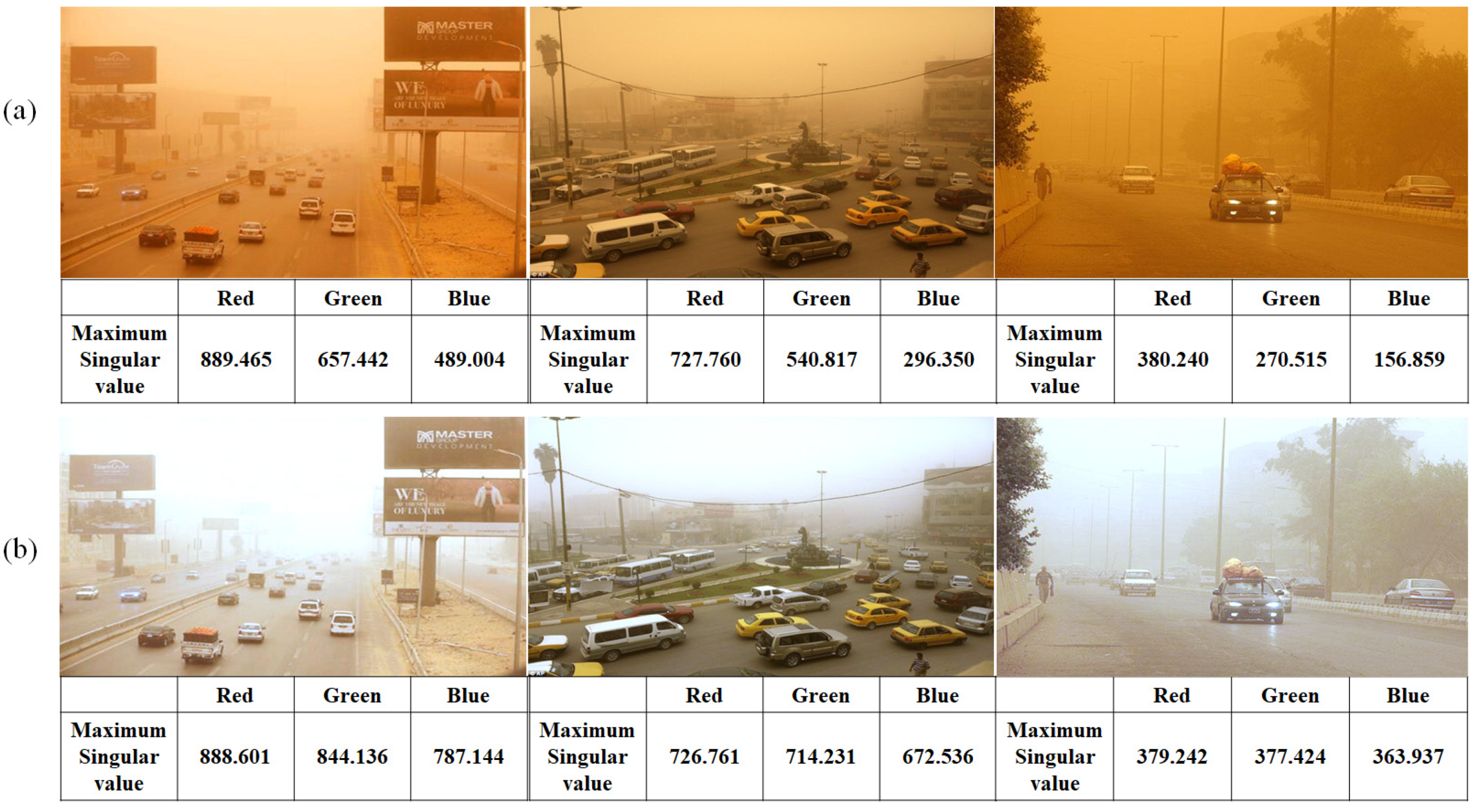
where ${\mathsf{\Sigma }}_{en}^c$ is the enhanced singular value. Using Equations (5)–(7), the color channels are balanced. If the color channel is degraded more, the image is more enhanced linearly and vice versa due to the normalized singular value being low. Figure 2 shows degraded duststorm images and their color-corrected images. As shown in Figure 2, the color corrected images using the proposed method have no color distortion, and these seem to be hazy images.

3.2. Estimate Adjustable Dark Channel Prior

The color-distorted image was corrected using the proposed method, and it seems to be a hazy image because its hazy ingredient is also increased by the compensated color channel. As known, a hazy image has a dimmed feature because of the haze particle. In general, a dehazing algorithm is used to enhance a hazy image. There are many dehazing algorithms, among them, the dark channel prior (DCP) method [1] is used often. The DCP estimates the dark region in an image. According to the DCP method, in a haze-free image, at least one channel among the three color channels is close to zero. Additionally, using the DCP estimates the back scatter light and transmission map [1]. The DCP method [1] is useful to enhance a hazy image. However, sometimes it improperly estimates the dark region, such as the sky region. Because of this, the enhanced image has an artifact result such as color distortion. The ordinary DCP is estimated as follows:

$${\mathrm{I}}_d\left(x\right)=\underset{c\in \left\{r,g,b\right\}}{\min }(\underset{y\in \mathsf{\Omega }\left(\mathrm{x}\right)}{\min }(\frac{{\mathrm{I}}_B^c\left(y\right)}{{\mathrm{A}}_{}^c}))$$

(8)

where ${\mathrm{A}}_{}^c$ is the back scatter light of the each balanced image’s color channel, $\mathsf{\Omega }\left(x\right)$ is the patch region (kernel size is 15 × 15), $\min$($·$) is the minimum operator to estimate the minimum pixel value on the color channels, and ${\mathrm{I}}_d^{}\left(x\right)$ is the dark channel image. The existing DCP method [1] estimates the dark region, but it is too bright in the sky region. To compensate this point, this work applied the bright channel prior (BCP) [29]. The BCP is described as follows [29]:

$${\mathrm{I}}_b\left(x\right)=\underset{c\in \left\{r,g,b\right\}}{\max }(\underset{y\in \mathsf{\Omega }\left(\mathrm{x}\right)}{\max }(\frac{{\mathrm{I}}_B^c\left(y\right)}{{\mathrm{A}}_b^c}))$$

(9)

where ${\mathrm{I}}_b\left(x\right)$ is the bright channel prior (BCP) [29], $\max (·)$ is the maximum operator to estimate the maximum pixel on the color channels of balanced image, and ${\mathrm{A}}_b^c$ is the back scatter light of bright channel prior on the balanced image. The BCP [29] is the converse measure with DCP and it estimates the bright region in an image. If the BCP [29] is applied in the process of estimating the DCP, the sky region is estimated darkly.

Therefore, this study proposes the adjustable DCP (ADCP), and it is described with the combination above Equations (8) and (9) as follows:

$${\mathrm{I}}_{ad}\left(x\right)=\frac{I_d\left(x\right)}{I_b\left(x\right)},$$

(10)

where ${\mathrm{I}}_{ad}\left(x\right)$ is the adjustable DCP (ADCP). In general, due to $I_d\left(x\right)$< $I_b\left(x\right)$, the intensity value of ${\mathrm{I}}_{ad}\left(x\right)$ is lower than that of ${\mathrm{I}}_d\left(x\right)$. However, if $I_d\left(x\right)$ and $I_b\left(x\right)$ are similar, ${\mathrm{I}}_{ad}\left(x\right)$ is bright and its intensity value is close to 1, then the halo effect can occur in the enhanced image. For this reason, the adaptive measure is applied in Equation (10), and it is described as follows:

$${\mathrm{I}}_{ad}\left(x\right)=\frac{\beta ·I_d\left(x\right)}{\max \left(\beta +\max (I_b\left(x\right), I_d\left(x\right)\right), {\beta }_0) },$$

(11)

$$\beta =\frac{\max \left(m\left(I_d\left(x\right)), m(I_b\left(x\right)\right)\right)}{\max \left(\min \left(m\left(I_d\left(x\right)), m( I_b\left(x\right)\right)\right), {\beta }_0\right)}$$

(12)

where ${\mathrm{I}}_{ad}\left(x\right)$ is the adjustable DCP (ADCP), and $\beta$ controls the intensity of ${\mathrm{I}}_{ad}\left(x\right)$. If $\beta$ is close to 0, ${\mathrm{I}}_{ad}\left(x\right)$ is bright and vice versa. Moreover, if $I_d\left(x\right)$ is close to zero, $\beta$ is close to infinite. ${\beta }_0$ is set to 0.1. Therefore, if $\beta$ is close to infinite, then $\beta +\max (I_b\left(x\right), I_d\left(x\right))$ is close to $\beta$ owing to $\beta$ is big enough than $\max (I_b\left(x\right), I_d\left(x\right))$. Consequently, $I_d\left(x\right)$ is maintained, but $\beta$ is close to infinite by multiplying $\beta$ on numerator. From Equations (11)–(12), the ADCP is able to estimate the dark region adjustably, though the image has the sky region. Additionally, the transmission map, which is the propagation path of the light, is estimated as follows [1]:

$$\mathrm{t}\left(x\right)=1-w · I_{ad}\left(x\right)$$

(13)

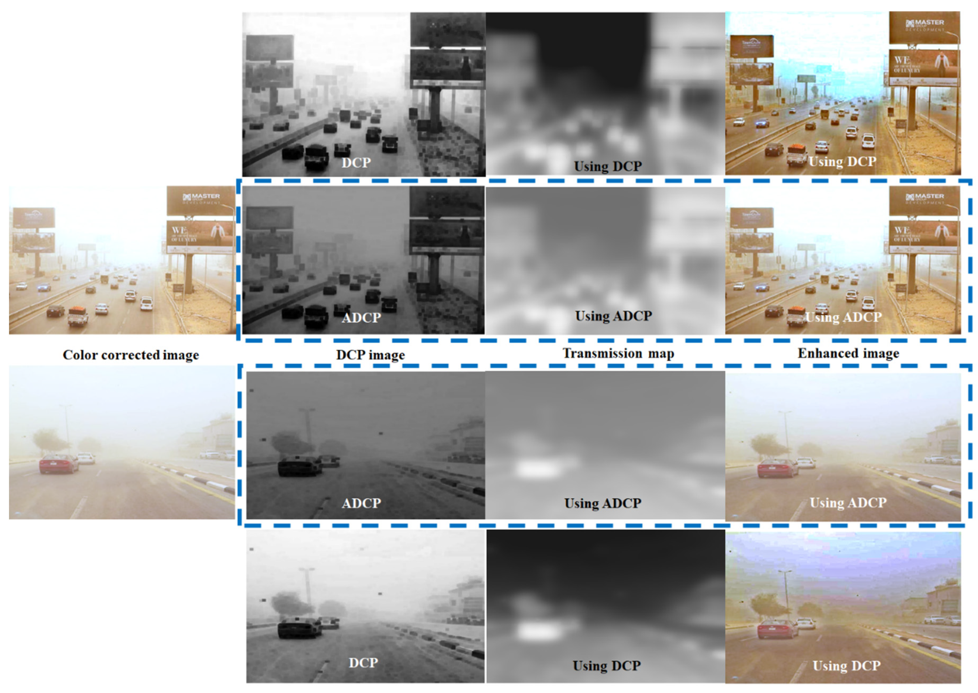
where $\mathrm{t}\left(x\right)$ is the transmission map. $w$ is set to 0.95 to apply the “aerial perspective” [1,30,31]. Additionally, to refine the transmission map, a guided image filter [10] is applied. Figure 3 shows the differences between the ordinary DCP [1] and its transmission map and enhanced image compared with the proposed ADCP, its transmission map and enhanced image of ADCP, respectively. As shown in Figure 3, the ordinary DCP [1] improperly estimates the dark region and this makes the halo effect is present in the enhanced image. However, the proposed ADCP estimates the dark region adjustably, and there is no halo effect in the enhanced image (The blue dotted line indicates the proposed method).

3.3. Image Enhancement

The degraded color channels are improved using the proposed color correction method. As the balanced duststorm image has similar features to the hazy image, this work estimates the ADCP and transmission map to dehaze the balanced image efficiently. The dehazing procedure is described as follows [16,17,18,19]:

$${\mathrm{J}}^c\left(x\right)=\frac{{\mathrm{I}}_B^c\left(x\right)-A^c}{\max \left(t\left(x\right), t_0\right)}+A^c$$

(14)

where ${\mathrm{J}}^c\left(x\right)$ is the enhanced image, ${\mathrm{I}}_B^c\left(x\right)$ is the color balanced image using the proposed method, $A_{}^c$ is the back scatter light using [1] on ${\mathrm{I}}_B^c\left(x\right)$, $t\left(x\right)$ is the transmission map, and $t_0$ is 0.1. When the duststorm image is enhanced due to the duststorm image having the degraded color channel, the color-corrected image and its back scatter light are used, and the transmission map is applied using ADCP. As shown in Figure 3, in the enhanced image using the proposed method, there is no halo effect or artifact color distortion. Additionally, to obtain the refined enhanced image, a guided image enhancement filter is used [10], and it is described as follows:

$${\mathrm{J}}_{GIF}^c\left(x\right)=\mathrm{GIF}\left\{{\mathrm{J}}^c\left(x\right), K, eps\right\}$$

(15)

$${\mathrm{J}}_{rei}^c\left(x\right)=\left({\mathrm{J}}^c\left(x\right)-{\mathrm{J}}_{GIF}^c\left(x\right)\right)· \gamma +J_{GIF}^c\left(x\right)$$

(16)

where $\mathrm{GIF}\{·\}$ is the guided image function, $\mathrm{K}$ is the kernel size set to 2, eps is set to ${0.4}^2$, $J_{GIF}^c\left(x\right)$ is the guided filtered image, $\gamma$ is set to 9, and ${\mathrm{J}}_{rei}^c\left(x\right)$ is the refined and enhanced image.

4. Experimental Results and Discussion

The color-degraded duststorm image was enhanced by the proposed color correction method and ADCP. As a result, the enhanced image seems natural. To express the superior point of the proposed method, this section compares the proposed method and the existing state-of-the-art methods objectively and subjectively. Additionally, a detection in adverse weather nature (DAWN) dataset [32] is used to compare these in various circumstances. The DAWN dataset [32] consists of 323 natural duststorm images.

4.1. Subjective Comparison

The subjective comparison consists of two steps. The first method is a comparison of the color correction, and the second step is a comparison of the enhanced image.

The first three color correction methods were used to compare the color correction. The Shi et al. method [8] corrected the degraded duststorm image using the mean shift of the color components, Shi et al. [12] improved the color distortion using the mean shift of the color ingredients and gamma correction, and Al Ameen [4] made the color balance using various constant thresholds.

Additionally, to express the difference between a lightly degraded duststorm image; a white (just dust and undegraded) and a severely distorted duststorm image; yellowish or reddish color cast, the comparison images are categorized into two types. One is the comparison of lightly degraded images and enhanced images using the existing methods and the proposed method. The other is a comparison of severely degraded images and enhanced images using the existing methods and the proposed method. In each category, 10 images were used.

Figure 4 and Figure 5 show the difference between the corrected images, which are degraded lightly and severely, respectively. As shown in Figure 4, a lightly degraded duststorm image is corrected appropriately, except for Al Ameen’s method [4]. Though Al Ameen’s method [4] has the color correction procedure, due to there being no adaptive threshold on the various image, the corrected image still has the color distortion. The Shi et al. method [8] has no bluish color distortion in some image. Al Ameen’s method [4] corrects the degraded duststorm image lightly in some images. The proposed method corrects the color appropriately.

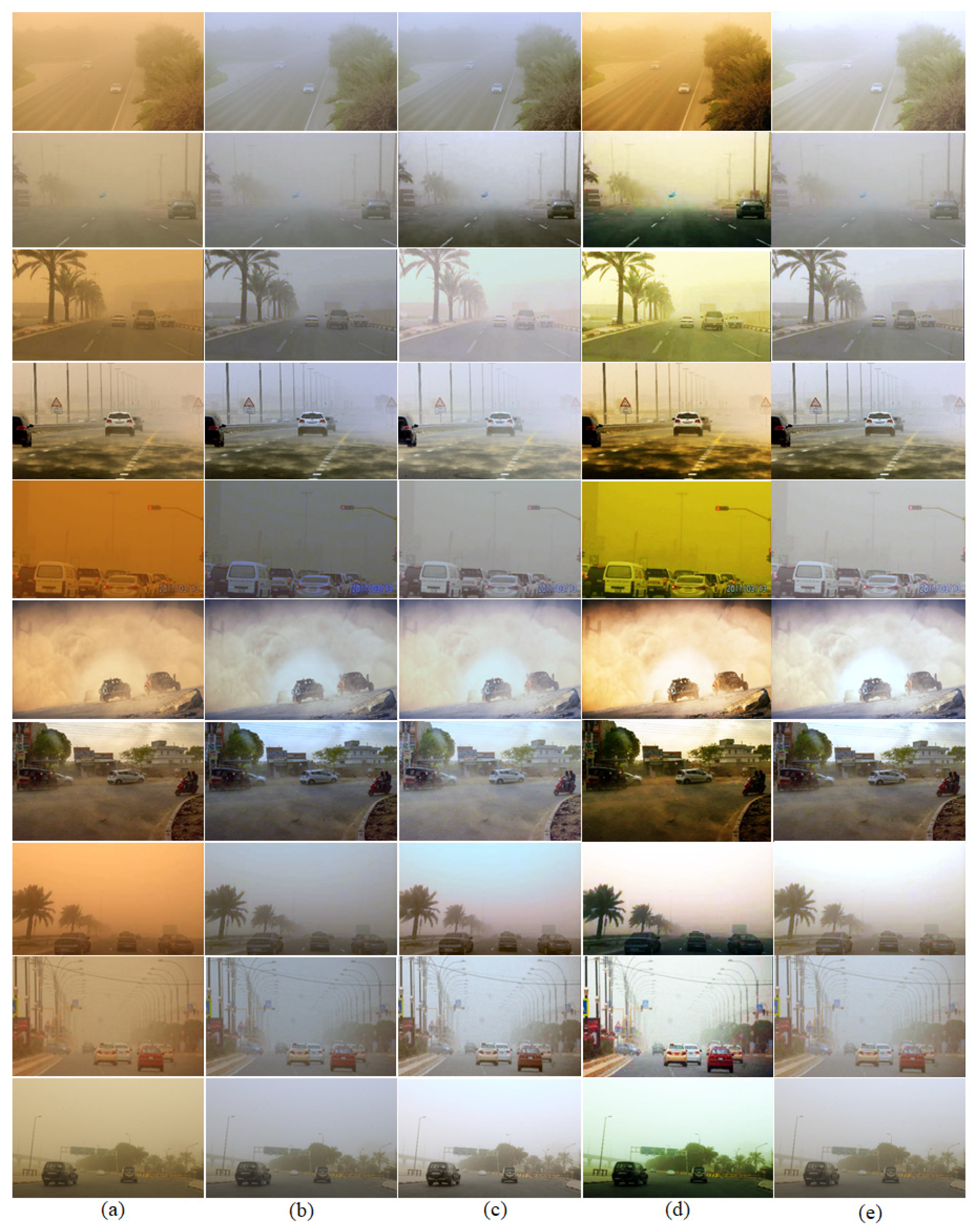
The correction of the lightly degraded duststorm images is not difficult. However, in the case of a severely degraded duststorm image, the existing methods have limitations. Figure 5 shows the severely distorted duststorm image and improved images using the existing methods and the proposed method. As shown in Figure 5, the existing color correction methods have the limitation of the improvement of the color. The Shi et al. method [8] has a bluish color degradation and partially greenish and yellowish color though this method has the color correction procedure. The corrected image using Shi et al. method [12] has a bluish and partially greenish color, though color correction is applied. Al Ameen [4] has various color degradations such as yellowish, orange, and reddish, though this method has the color balancing procedure applied. The proposed method makes the color channel balance appropriately without color degradation.

As shown in Figure 4 and Figure 5, the corrected results are different for variously degraded duststorm images. To obtain a well-corrected duststorm image, an adaptive color correction procedure is needed; if not, the corrected image also has a color shift or degraded effect.

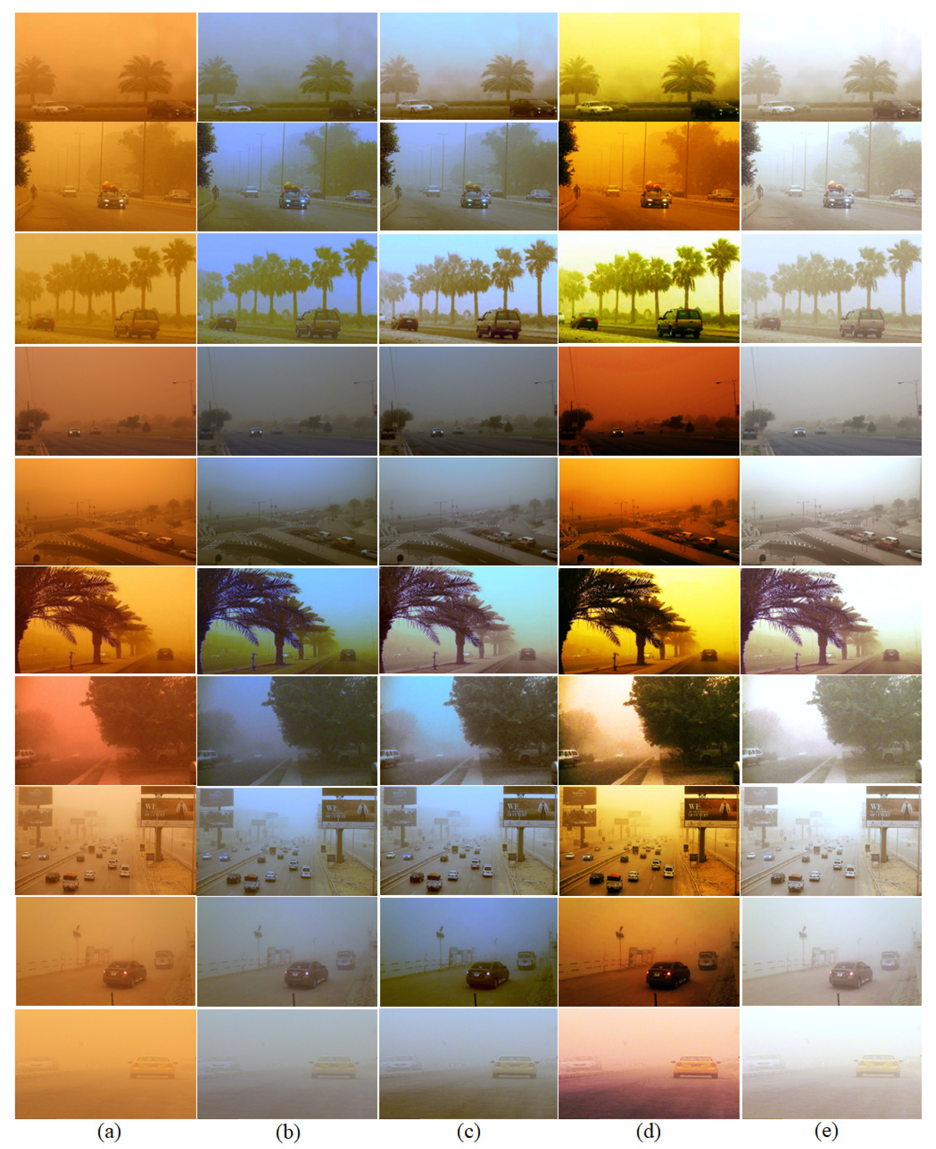
The duststorm image has the similar obtaining process as the hazy image. For this reason, to compare the enhanced image, existing dehazing methods were used. Figure 6 and Figure 7 show the enhanced duststorm image comparison with existing methods and the proposed method. He et al.’s method [1] used the DCP to enhance a hazy image. Meng et al. used compensated DCP [2] to improve the hazy image, Ren et al. applied CNN to enhance the hazy image [15], Gao et al. used RBCP to enhance the duststorm image [7], and Al Ameen applied tri thresholds to improve the degraded duststorm image [4].

Figure 6 shows the enhanced duststorm image that is lightly degraded. As shown in Figure 6, the existing dehazing methods (including those by He et al. [1], Meng et al. [2], and Ren et al. [15]) still have the halo effect and color shift. Gao et al.’s method [7] has no color shift, but the hazy effect is still present. Al Ameen’s method [4] has the color shift, though this method has the color correction step. However, the lightly color shifted images seem to be well enhanced in some images. The dehazing process is well applied in the enhanced images using the proposed method except for the thick hazy region.

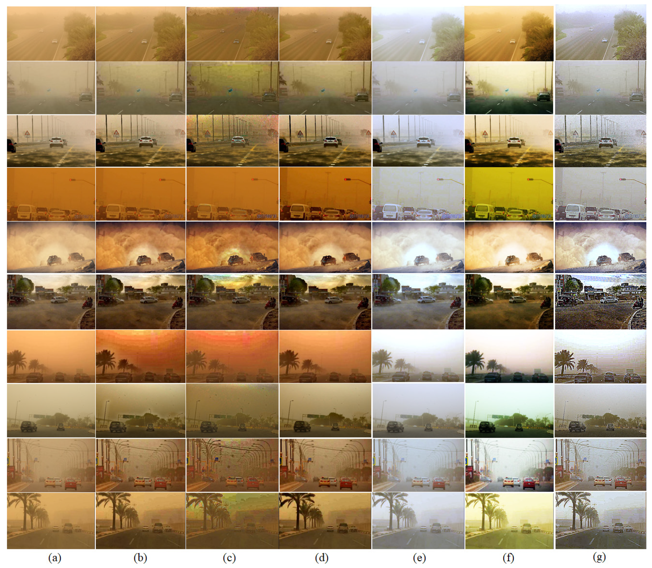
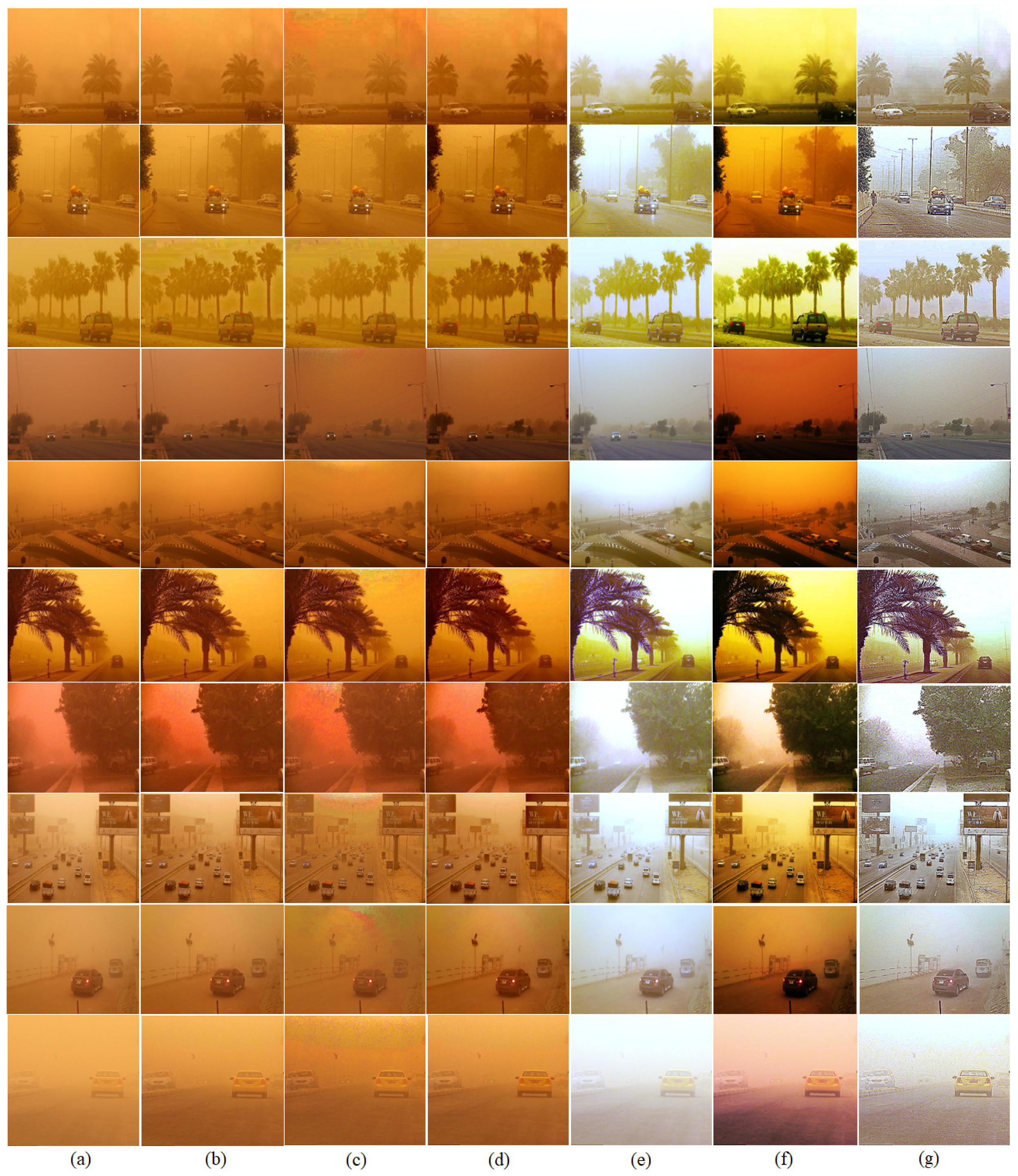
Figure 7 shows the severely degraded duststorm images and the enhanced images. As shown in Figure 7, the enhanced images just using the dehazing algorithms (He et al. [1], Meng et al. [2], and Ren et al. [15]) still have the halo effect. Though Gao et al.’s method [7] has the color correction step, a yellowish color shift is shown in some images. Al Ameen’s method [4] has the color shift, though this method has the color correction procedure. The proposed method has no color shift and is enhanced appropriately except for the thick haze regions.

As shown through Figure 4, Figure 5, Figure 6, Figure 7, an image adaptive color correction procedure and a dehazing procedure are needed to enhance the duststorm image naturally. Additionally, the proposed method is able to enhance the duststorm image (both the lightly and severely degraded images), and it is superior to the existing methods.

4.2. Objective Comparison

Through Figure 4, Figure 5, Figure 6 and Figure 7, the images enhanced with the existing methods and the proposed method were compared, and as a result, the proposed method outperforms the existing methods. Additionally, for an objective comparison the natural image quality evaluator (NIQE) measure [33], underwater image quality measure (UIQM) [34], haziness degree evaluator (HDE) [35], and fog aware density evaluator (FADE) [36] were used. The NIQE measures the naturalism of an image; if the NIQE score is low, it indicates a well-enhanced image. Additionally, the UIQM [34] is used in the improved underwater image assessment. In general, an underwater image is a degraded color channel by the attenuation of light. The duststorm image has similar feature to an underwater image on a degraded color channel. The UIQM [34] assesses the contrast, colorfulness, and sharpness of an image. If the UIQM measure is a high score, then it indicates a well-enhanced image. Additionally, the HDE [35] and FADE [36] measure the haze density of an enhanced image. If the image is dehazed well, both scores are low and vice versa.

Table 1. The comparison of the NIQE [33] scores from Figure 6 (If the score is low, the image is well enhanced. The lowest are indicated in bold).

	Input	He et al. [1]	Meng et al. [2]	Ren et al. [15]	Gao et al. [7]	Al Ameen [4]	Proposed Method
	19.346	19.252	19.186	19.202	19.200	18.947	15.496
	19.896	19.824	19.694	19.798	19.884	19.789	19.290
	19.304	19.036	17.475	18.940	19.220	19.141	14.670
	21.091	21.053	21.832	20.829	20.354	20.425	16.682
	19.755	19.532	19.314	19.628	19.691	19.396	14.026
	21.608	20.770	22.205	21.236	21.084	23.200	15.248
	20.841	21.287	21.475	21.118	20.939	20.639	18.374
	19.844	19.707	19.624	19.768	19.824	19.762	17.067
	19.483	18.933	18.081	18.889	19.371	18.970	16.119
	20.419	20.106	21.001	20.087	20.236	19.982	16.272
AVG	20.159	19.950	19.989	19.950	19.980	20.025	16.324

shows the NIQE [33] scores from Figure 6. Figure 6 shows the lightly degraded duststorm image and enhanced images. As shown in Table 1, the enhanced image using just the dehazing algorithms has low quality and it has a high NIQE score. Gao et al.’s method [7] has the color correction step, and the enhanced image shows balance in the color channel. However, in the NIQE score, it is higher than that of the He et al. [1] method in some images, though the He et al. method [1] has no color correction procedure, and the enhanced image still has the halo effect. The image enhanced using Al Ameen’s method [4], in some images, has no halo effect in Figure 6. However, in the NIQE score, it is higher than the other dehazing methods such as those of He et al. [1], Meng et al. [2], and Ren et al. [15] in some images. The images enhanced using the proposed method have low NIQE scores. As shown in Table 1, to enhance the duststorm image naturally, an image adaptive color correction step and a dehazing algorithm are considered.

Table 2. The comparison of the UIQM [34] scores from Figure 6 (If the score is high, the image is well enhanced. The highest are indicated in bold).

	Input	He et al. [1]	Meng et al. [2]	Ren et al. [15]	Gao et al. [7]	Al Ameen [4]	Proposed Method
	0.551	0.630	0.691	0.701	0.652	0.906	1.639
	0.298	0.389	0.527	0.518	0.326	0.798	0.940
	0.941	1.236	1.441	1.436	1.020	1.161	1.771
	0.517	0.552	0.605	0.871	0.695	0.828	1.391
	0.569	0.849	0.981	0.870	0.628	0.794	1.986
	1.330	1.518	1.496	1.524	1.363	1.583	1.702
	0.548	0.809	0.622	0.687	0.627	0.943	1.940
	0.519	0.839	0.767	0.777	0.563	0.902	1.887
	0.573	0.973	1.242	1.007	0.671	1.009	1.582
	0.572	0.773	0.710	0.930	0.655	0.773	1.548
AVG	0.642	0.857	0.908	0.932	0.720	0.970	1.639

shows the UIQM [34] scores on Figure 6, which are lightly degraded duststorm images and enhanced images using the existing methods and the proposed method. As shown in Table 2, due to the dehazing methods having no color correction step, these have low UIQM scores. Though Gao et al.’s method [7] has the color correction procedure, the UIQM scores of the existing dehazing methods are higher than that of Gao et al.’s [7] results in some images. Al Ameen’s method [4] has high UIQM scores in comparison with the other dehazing methods in some images. The UIQM scores of the enhanced images using the proposed method are higher than those of the other methods.

Table 3. The comparison of the HDE [35] scores from Figure 6 (If the score is low, the image is well enhanced. The lowest are indicated in bold).

	Input	He et al. [1]	Meng et al. [2]	Ren et al. [15]	Gao et al. [7]	Al Ameen [4]	Proposed Method
	0.896	0.860	0.805	0.828	0.950	0.832	0.726
	0.939	0.908	0.840	0.882	0.960	0.889	0.928
	0.847	0.782	0.698	0.686	0.885	0.771	0.478
	0.807	0.790	0.803	0.606	0.940	0.714	0.834
	0.915	0.844	0.832	0.856	0.958	0.904	0.758
	0.752	0.589	0.630	0.568	0.800	0.615	0.115
	0.878	0.714	0.809	0.818	0.948	0.909	0.718
	0.906	0.824	0.818	0.836	0.941	0.895	0.716
	0.897	0.802	0.761	0.771	0.943	0.920	0.696
	0.884	0.823	0.809	0.757	0.944	0.884	0.733
AVG	0.872	0.794	0.781	0.761	0.927	0.833	0.670

shows the HDE [35] scores on Figure 6. If the enhanced image has a low density of haze, then the score is low. As shown in Table 3, the existing dehazing methods have lower scores than the input image. The proposed method has low values.

Table 4. The comparison of the FADE [36] scores from Figure 6 (If the score is low, the image is well enhanced. The lowest are indicated in bold).

	Input	He et al. [1]	Meng et al. [2]	Ren et al. [15]	Gao et al. [7]	Al Ameen [4]	Proposed Method
	1.667	1.310	0.808	1.143	5.522	1.303	0.572
	3.042	2.154	1.215	1.824	8.682	2.780	1.793
	0.746	0.499	0.305	0.412	1.126	0.591	0.175
	1.019	0.965	0.999	0.809	3.146	0.891	1.041
	1.548	0.824	0.645	0.929	4.224	1.659	0.441
	0.408	0.259	0.255	0.258	0.627	0.283	0.128
	1.280	0.614	0.687	0.962	4.644	3.110	0.703
	2.048	1.035	0.763	1.252	4.888	2.573	0.468
	0.913	0.558	0.418	0.566	2.243	1.487	0.257
	1.528	1.092	0.913	1.027	4.533	1.712	0.775
AVG	1.420	0.931	0.701	0.918	3.964	1.639	0.635

shows the FADE [36] scores of Figure 6. If the image is enhanced well, the score is low. As shown in Table 4, the scores of Al Ameen’s method [4] are higher than that of the dehazing methods though the images enhanced using this method have no color distortion. The scores of the proposed method are lower than that of the other methods.

Table 5. The comparison of the NIQE [33] scores from Figure 7 (If the score is low, the image is well enhanced. The lowest are indicated in bold).

	Input	He et al. [1]	Meng et al. [2]	Ren et al. [15]	Gao et al. [7]	Al Ameen [4]	Proposed Method
	19.969	19.930	19.997	19.940	20.064	19.825	18.941
	21.066	21.101	20.804	21.324	20.174	21.203	14.470
	20.157	20.202	20.102	20.130	19.901	19.515	17.705
	19.585	19.569	19.523	19.518	19.513	19.548	18.385
	19.898	19.863	19.699	19.724	19.811	19.772	15.903
	19.417	19.378	19.756	19.331	18.565	19.207	15.752
	20.658	20.881	21.030	20.666	20.398	20.553	16.175
	20.469	20.302	20.167	20.248	20.093	19.902	14.293
	20.265	20.243	20.250	20.212	20.183	20.118	18.194
	19.510	19.373	18.908	19.337	19.456	19.258	15.743
AVG	20.099	20.084	20.024	20.043	19.816	19.890	16.556

shows the NIQE [33] scores on Figure 7. Figure 7 shows the severely degraded image and enhanced images. Gao et al.’s method [7] has the color balance step, but it has no compensation on the rare color channel. Therefore, the images enhanced using Gao et al.’s method have high NIQE [33] scores. Sometimes, Gao et al.’s [7] NIQE scores are higher than the dehazing method’s NIQE scores. Al Ameen’s method [4] has high NIQE scores in some of the images due to it having no image adaptive color balancing step and dehazing procedure. The images enhanced using the proposed method have low NIQE scores. As shown through Table 5, a color channel compensation procedure and an adaptive dehazing step are needed to enhance the severely degraded duststorm image.

Table 6. The comparison of the UIQM [34] scores from Figure 7 (If the score is high, the image is well enhanced. The highest are indicated in bold).

	Input	He et al. [1]	Meng et al. [2]	Ren et al. [15]	Gao et al. [7]	Al Ameen [4]	Proposed Method
	0.364	0.386	0.328	0.437	0.523	0.678	1.123
	0.907	0.919	0.932	1.123	1.126	1.264	1.851
	0.477	0.493	0.468	0.630	0.739	1.003	1.398
	0.381	0.434	0.506	0.620	0.474	0.753	1.406
	0.839	0.883	0.924	1.083	1.009	1.211	2.076
	0.890	0.910	0.939	1.067	1.060	1.182	1.625
	0.615	0.773	0.690	0.814	0.777	1.140	1.729
	0.797	0.888	0.910	0.951	0.927	1.205	1.911
	0.356	0.418	0.434	0.553	0.502	0.823	1.348
	0.377	0.611	0.869	0.659	0.496	0.736	1.535
AVG	0.600	0.672	0.700	0.794	0.763	1.000	1.600

shows the UIQM [34] scores from Figure 7, which consists of the severely degraded duststorm images and the images enhanced using the existing methods and the proposed method. As shown in Table 6, the UIQM scores using just the dehazing methods are low because of the limitation of the color correction. Al Ameen’s method [4] has higher UIQM scores than Gao et al.’s method [7], though it has color degradation in some of the enhanced images. The UIQM scores of the proposed method have a higher value than the other methods, because the color balancing procedure and dehazing step are applied appropriately to the image.

Table 7. The comparison of the HDE [35] scores from Figure 7 (If the score is low, the image is well enhanced. The lowest are indicated in bold).

	Input	He et al. [1]	Meng et al. [2]	Ren et al. [15]	Gao et al. [7]	Al Ameen [4]	Proposed Method
	0.795	0.750	0.762	0.612	0.889	0.709	0.897
	0.627	0.611	0.612	0.285	0.754	0.339	0.393
	0.657	0.516	0.629	0.332	0.760	0.573	0.816
	0.858	0.845	0.803	0.776	0.944	0.733	0.846
	0.664	0.648	0.625	0.438	0.783	0.448	0.412
	0.599	0.570	0.542	0.289	0.706	0.378	0.482
	0.783	0.659	0.746	0.553	0.892	0.714	0.478
	0.796	0.722	0.717	0.617	0.889	0.656	0.543
	0.862	0.842	0.804	0.773	0.950	0.776	0.860
	0.882	0.832	0.771	0.822	0.969	0.906	0.766
AVG	0.752	0.700	0.701	0.550	0.854	0.623	0.649

shows the HDE [35] scores from Figure 7. As shown in Table 7, the existing dehazing methods have lower HDE scores than the scores of the input images. The result scores of Al Ameen’s method [4] are lower than that of the dehazing methods in some image, though this method has no dehazing step. The proposed method has lower scores than that of the other methods in some image.

Table 8. The comparison of the FADE [36] scores from Figure 7 (If the score is low, the image is well enhanced. The lowest are indicated in bold).

	Input	He et al. [1]	Meng et al. [2]	Ren et al. [15]	Gao et al. [7]	Al Ameen [4]	Proposed Method
	1.229	1.114	0.959	1.010	3.181	1.202	1.518
	0.507	0.489	0.446	0.405	1.100	0.396	0.262
	0.765	0.628	0.675	0.644	1.184	0.888	0.678
	1.046	0.961	0.774	0.770	3.896	0.758	0.572
	0.502	0.465	0.417	0.373	1.178	0.381	0.239
	0.601	0.554	0.502	0.507	0.947	0.539	0.351
	0.621	0.468	0.498	0.482	1.419	0.541	0.310
	0.714	0.573	0.463	0.533	1.588	0.511	0.290
	1.192	1.087	0.838	0.917	3.877	0.913	0.792
	0.884	0.661	0.492	0.621	5.226	1.406	0.560
AVG	0.806	0.700	0.606	0.626	2.360	0.754	0.557

shows the FADE [36] scores from Figure 7. The existing dehazing methods have low scores though these methods have degraded images. The proposed method has lower scores than that of the other methods.

Through Table 3, Table 4, Table 7 and Table 8, the scores of haze density are not an appropriate measure of the duststorm image. Because the HDE [35] and FADE [36] measure just the hazy density of image, the enhanced image has color distortion, but the score is low.

Table 9. The comparison of the NIQE [33] average scores on sample images (Figure 6 and Figure 7) and the DWAN dataset [32] (The lowest scores are indicated in bold).

	Input	He et al. [1]	Meng et al. [2]	Ren et al. [15]	Gao et al. [7]	Al Ameen [4]	Proposed Method
AVG (20)	20.129	20.017	20.006	19.996	19.898	19.958	16.440
AVG (373)	20.032	19.863	19.698	19.892	19.931	19.803	16.988

and

Table 10. The comparison of the UIQM [34] average scores on the sample images (Figure 6 and Figure 7) and DWAN dataset [32] (If the score is high, the image is enhanced well. The highest scores are indicated in bold).

	Input	He et al. [1]	Meng et al. [2]	Ren et al. [15]	Gao et al. [7]	Al Ameen [4]	Proposed Method
AVG (20)	0.621	0.764	0.804	0.863	0.742	0.985	1.619
AVG (323)	0.600	0.806	0.928	0.840	0.671	0.938	1.615

show the average values of the NIQE measure [33] and the UIQM [34] on the duststorm image dataset [32]. In Table 9, the average NIQE scores of Gao et al. [7] and Al Ameen [4] are lower than the results of the dehazing methods on the sample images (Figure 6 and Figure 7). Additionally, the average NIQE score on the dataset [32] in the case of Gao et al.’s method [7] is higher than just the dehazing methods. The proposed method has the lowest average NIQE value on the sample images (Figure 6 and Figure 7) and DAWN dataset [32].

Additionally, the average UIQM scores are shown in Table 10. As shown in Table 10, the average UIQM score of Al Ameen [4] is higher than just the dehazing methods on the sample images (Figure 6 and Figure 7) and dataset [32]. The proposed method has the highest score on the sample images (Figure 6 and Figure 7) and dataset [32].

Table 11. The comparison of the HDE [35] average scores on the sample images (Figure 6 and Figure 7) and DWAN dataset [32] (If the score is low, the image is enhanced well. The lowest scores are indicated in bold).

	Input	He et al. [1]	Meng et al. [2]	Ren et al. [15]	Gao et al. [7]	Al Ameen [4]	Proposed Method
AVG (20)	0.812	0.747	0.741	0.655	0.890	0.728	0.660
AVG (323)	0.851	0.780	0.756	0.746	0.888	0.781	0.724

and

Table 12. The comparison of the FADE [36] average scores on the sample images (Figure 6 and Figure 7) and DWAN dataset [32] (If the score is low, the image is enhanced well. The lowest scores are indicated in bold).

	Input	He et al. [1]	Meng et al. [2]	Ren et al. [15]	Gao et al. [7]	Al Ameen [4]	Proposed Method
AVG (20)	1.113	0.815	0.654	0.772	3.161	1.196	0.596
AVG (323)	2.476	1.358	0.798	1.349	3.648	1.675	0.594

show the average haze density scores of Figure 6 and Figure 7 and the DWAN [32] dataset. Table 11 shows the HDE [35] score on the result images. The Al Ameen method [4] has a lower score than that of the existing dehazing methods on the sample images (Figure 6 and Figure 7). The existing dehazing methods have a lower score than that of the other methods on the dataset [32], though these methods have a color cast. The proposed method has a lower score than the other methods without an artificial color cast.

Additionally, Table 12 shows the FADE [36] scores on the result images. As shown in Table 12, the existing dehazing methods have low scores than Gao et al. [7] and Al Ameen [4] methods, though these methods have a color cast in the enhanced image. The proposed method has a low score without a color cast.

Through Table 1, Table 2, Table 3, Table 4, Table 5, Table 6, Table 7, Table 8, Table 9, Table 10, Table 11 and Table 12 and Figure 4, Figure 5, Figure 6 and Figure 7, the image adaptive color correction step and dehazing procedure are considered to enhance the duststorm image naturally. As the proposed method has the image adaptive color balancing step and dehazing procedure, the images enhanced using the proposed method have no halo effect, and it is shown well in the objective measures.

5. Conclusions

In this study, to enhance a duststorm images naturally, two steps were proposed. The first step is color correction using the normalized singular value. The singular value is able to express the image’s feature such as dark or bright. In a duststorm image, the red channel’s singular value is high because the red channel is bright. However, the blue channel is dark, and its singular value is low if the duststorm image is degraded. Consequently, if the singular value of the color channel is uniform, the degraded duststorm image can be balanced adaptively. The second step of the proposed method is dehazing the balanced image because the corrected image seems to be a hazy image. In general, the DCP method [1] is used to dehaze the image. However, the DCP method [1] improperly estimates the dark region especially in the sky region. Therefore, this study proposed the adjustable DCP (ADCP) using BCP [29]. The proposed method is superior to the state-of-the-art methods objectively and subjectively, as shown by the experimental results. The proposed duststorm image enhancement method will contribute to various degraded image enhancement areas. The next work will obtain the accommodative color correction method and adaptive transmission map with a hazy density adaptive transmission map, which estimates the density of a hazy region using the depth of an image. If the adaptive dehazing method applies the image’s depth in an image depicting traffic, though the object looks dimmed, the plate number can be clearly shown.

References

- He, K.; Sun, J.; Tang, X. Single image haze removal using dark channel prior. IEEE Trans. Pattern Anal. Mach. Intell. 2010, 33, 2341–2353. [Google Scholar]
- Meng, G.; Wang, Y.; Duan, J.; Xiang, S.; Pan, C. Efficient image dehazing with boundary constraint and contextual regularization. In Proceedings of the IEEE International Conference on Computer Vision, Sydney, Australia, 1–8 December 2013. [Google Scholar]
- Zhu, Q.; Mai, J.; Shao, L. A fast single image haze removal algorithm using color attenuation prior. IEEE Trans. Image Process. 2015, 24, 3522–3533. [Google Scholar]
- Al-Ameen, Z. Visibility enhancement for images captured in dusty weather via tuned tri-threshold fuzzy intensification operators. Int. J. Intell. Syst. Appl. 2016, 8, 10. [Google Scholar] [CrossRef] [Green Version]
- Naseeba, T.; Harish Binu, K.P. Visibility Restoration of Single Hazy Images Captured in Real-World Weather Conditions. 2016.
- Kwok, N.; Wang, D.; Jia, X.; Chen, S.; Fang, G.; Ha, Q. Gray world based color correction and intensity preservation for image enhancement. In Proceedings of the 2011 4th International Congress on Image and Signal Processing, Shanghai, China, 15–17 October 2011; Volume 2. [Google Scholar]
- Gao, G.; Lai, H.; Jia, Z.; Liu, Y.Q.; Wang, Y. Sand-dust image restoration based on reversing the blue channel prior. IEEE Photonics J. 2020, 12, 1–16. [Google Scholar] [CrossRef]
- Shi, Z.; Feng, Y.; Zhao, M.; Zhang, E.; He, L. Let you see in duststorm weather: A method based on halo-reduced dark channel prior dehazing for sand-dust image enhancement. IEEE Access 2019, 7, 116722–116733. [Google Scholar] [CrossRef]
- Huo, J.-Y.; Chang, Y.-L.; Wang, J.; Wei, X.-X. Robust automatic white balance algorithm using gray color points in images. IEEE Trans. Consum. Electron. 2006, 52, 541–546. [Google Scholar]
- He, K.; Sun, J.; Tang, X. Guided image filtering. IEEE Trans. Pattern Anal. Mach. Intell. 2012, 35, 1397–1409. [Google Scholar] [CrossRef]
- Cheng, Y.; Jia, Z.; Lai, H.; Yang, J.; Kasabov, N.K. A fast sand-dust image enhancement algorithm by blue channel compensation and guided image filtering. IEEE Access 2020, 8, 196690–196699. [Google Scholar] [CrossRef]
- Shi, Z.; Feng, Y.; Zhao, M.; Zhang, E.; He, L. Normalised gamma transformation-based contrast-limited adaptive histogram equalisation with colour correction for sand–dust image enhancement. IET Image Process. 2019, 14, 747–756. [Google Scholar] [CrossRef]
- Wang, A.; Wang, W.; Liu, J.; Gu, N. AIPNet: Image-to-image single image dehazing with atmospheric illumination prior. IEEE Trans. Image Process. 2018, 28, 381–393. [Google Scholar] [CrossRef]
- Zhang, J.; Tao, D. FAMED-Net: A fast and accurate multi-scale end-to-end dehazing network. IEEE Trans. Image Process. 2019, 29, 72–84. [Google Scholar] [CrossRef] [PubMed] [Green Version]
- Ren, W.; Liu, S.; Zhang, H.; Pan, J.; Cao, X.; Yang, M.-H. Single image dehazing via multi-scale convolutional neural networks. In European Conference on Computer Vision; Springer: Cham, Switzerland, 2016. [Google Scholar]
- Fattal, R. Single image dehazing. ACM Trans. Graph. (TOG) 2008, 27, 1–9. [Google Scholar] [CrossRef]
- Narasimhan, S.G.; Nayar, S.K. Chromatic framework for vision in bad weather. In Proceedings of the IEEE Conference on Computer Vision and Pattern Recognition. CVPR 2000 (Cat. No. PR00662), Hilton Head, SC, USA, 15 June 2020; Volume 1. [Google Scholar]
- Narasimhan, S.G.; Nayar, S.K. Vision and the atmosphere. Int. J. Comput. Vis. 2002, 48, 233–254. [Google Scholar] [CrossRef]
- Tan, R.T. Visibility in bad weather from a single image. In Proceedings of the 2008 IEEE Conference on Computer Vision and Pattern Recognition, Anchorage, AK, USA, 23–28 June 2008. [Google Scholar]
- Shepherd, G.; Terradellas, E.; Baklanov, A.; Kang, U.; Sprigg, W.; Nickovic, S.; Boloorani, A.D.; Al-Dousari, A.; Basart, S.; Benedetti, A.; et al. Global Assessment of Sand and Dust Storms; United Nations Environment Programme: Nairobi, Kenya, 2016. [Google Scholar]
- Gillett, D.; Morales, C. Environmental factors affecting dust emission by wind erosion. Sahar. Dust. 1979, 71–94. [Google Scholar]
- Ancuti, C.O.; Ancuti, C.; De Vleeschouwer, C.; Bekaert, P. Color balance and fusion for underwater image enhancement. IEEE Trans. Image Process. 2017, 27, 379–393. [Google Scholar] [CrossRef] [Green Version]
- Sadek, R.A. SVD based image processing applications: State of the art, contributions and research challenges. arXiv 2012, arXiv:1211.7102. [Google Scholar]
- Cao, L. Singular Value Decomposition Applied to Digital Image Processing; Division of Computing Studies, Arizona State University Polytechnic Campus, Mesa, Arizona State University polytechnic Campus: Mesa, AZ, USA, 2006; pp. 1–15. [Google Scholar]
- Ogden, C.J.; Huff, T. The Singular Value Decomposition and It Ys Applications in Image Processing; Lin. Algebra-Maths-45, College of Redwoods: Eureka, CA, USA, 1997. [Google Scholar]
- Tripathi, P.; Garg, R.D. Comparative Analysis of Singular Value Decomposition and Eigen Value Decomposition Based Principal Component Analysis for Earth and Lunar Hyperspectral Image. In Proceedings of the 2021 11th Workshop on Hyperspectral Imaging and Signal Processing: Evolution in Remote Sensing (WHISPERS), Amsterdam, The Netherlands, 24–26 March 2021. [Google Scholar]
- Halder, N.; Roy, D.; Mitra, A. Low-light Video Enhancement with SVD-DWT Algorithm for Multimedia Surveillance Network. Curr. Trends Signals Processing 2020, 10, 43–51. [Google Scholar]
- Li, P.; Wang, H.; Li, X.; Zhang, C. An image denoising algorithm based on adaptive clustering and singular value decomposition. IET Image Process. 2021, 15, 598–614. [Google Scholar] [CrossRef]
- Shi, Z.; Zhu, M.M.; Guo, B.; Zhao, M.; Zhang, C. Nighttime low illumination image enhancement with single image using bright/dark channel prior. EURASIP J. Image Video Process. 2018, 2018, 13. [Google Scholar] [CrossRef] [Green Version]
- Goldstein, E.B. Sensation and Perception; Wadsworth: Belmont, CA, USA; p. 1980.
- Preetham, A.J.; Shirley, P.; Smits, B. A practical analytic model for daylight. In Proceedings of the 26th Annual Conference on Computer Graphics and Interactive Techniques, New York, NY, USA, 1 July 1999. [Google Scholar]
- Kenk, M.A.; Hassaballah, M. DAWN: Vehicle Detection in Adverse Weather Nature Dataset. arXiv 2020, arXiv:2008.05402. [Google Scholar]
- Mittal, A.; Soundararajan, R.; Bovik, A.C. Making a “completely blind” image quality analyzer. IEEE Signal Process. Lett. 2012, 20, 209–212. [Google Scholar] [CrossRef]
- Panetta, K.; Gao, C.; Agaian, S. Human-visual-system-inspired underwater image quality measures. IEEE J. Ocean. Eng. 2015, 41, 541–551. [Google Scholar] [CrossRef]
- Ngo, D.; Lee, G.-D.; Kang, B. Haziness Degree Evaluator: A Knowledge-Driven Approach for Haze Density Estimation. Sensors 2021, 21, 3896. [Google Scholar] [CrossRef] [PubMed]
- Choi, L.K.; You, J.; Bovik, A. Referenceless prediction of perceptual fog density and perceptual image defogging. IEEE Trans. Image Processing 2015, 24, 3888–3901. [Google Scholar] [CrossRef] [PubMed]
Figure 1.
The images’s mean value and their singular values: (a) The not degraded duststorm image’s mean value and its singular value on each color channel; (b) The degraded duststorm image’s mean value and its singular value.
Figure 2.
The degraded duststorm images (a) and their color corrected images (b). (The tables below the images indicate each channel’s maximum singular value).
Figure 3.
The comparison with DCP [1] and the proposed ADCP and their transmission map and enhanced image (Blue dotted line indicates the proposed method).
Figure 4.
The comparison with state-of-the-art color correction methods and the proposed method: (a) Input image; (b) Shi et al. [8]; (c) Shi et al. [12]; (d) Al Ameen [4]; (e) Proposed method.
Figure 5.
The comparison with state-of-the-art color correction methods and the proposed method on severely degraded duststorm images: (a) Input image; (b) Shi et al. [8]; (c) Shi et al. [12]; (d) Al Ameen [4]; (e) Proposed method.
Figure 6.
The comparison of the enhanced image with state-of-the-art methods and the proposed method on lightly degraded duststorm images: (a) Input image; (b) He et al. [1]; (c) Meng et al. [2]; (d) Ren et al. [15]; (e) Gao et al. [7]; (f) Al Ameen [4]; (g) Proposed method.
Figure 7.
The comparison of the enhanced image with state-of-the-art methods and the proposed method on severely degraded duststorm images: (a) Input image; (b) He et al. [1]; (c) Meng et al. [2]; (d) Ren et al. [15]; (e) Gao et al. [7]; (f) Al Ameen [4]; (g) Proposed method.