Resilient Predictive Control Coupled with a Worst-Case Scenario Approach for a Distributed-Generation-Rich Power Distribution Grid

Abstract

In a context of accelerating deployment of distributed generation in power distribution grid, this work proposes an answer to an important and urgent need for better management tools in order to ‘intelligently’ operate these grids and maintain quality of service. To this aim, a model-based predictive control (MPC) strategy is proposed, allowing efficient re-routing of power flows using flexible assets, while respecting operational constraints as well as the voltage constraints prescribed by ENEDIS, the French distribution grid operator. The flexible assets used in the case study—a low-voltage power distribution grid in southern France—are a biogas plant and a water tower. Non-parametric machine-learning-based models, i.e., Gaussian process regression (GPR) models, are developed for intraday forecasting of global horizontal irradiance (GHI), grid load, and water demand, to better anticipate emerging constraints. The forecasts’ quality decreases as the forecast horizon grows longer, but quickly stabilizes around a constant error value. Then, the impact of forecasting errors on the performance of the control strategy is evaluated, revealing a resilient behaviour where little degradation is observed in terms of performance and computation cost. To enhance the strategy’s resilience and minimise voltage overflow, a worst-case scenario approach is proposed for the next time step and its contribution is examined. This is the main contribution of the paper. The purpose of the min–max problem added upstream of the main optimisation problem is to both anticipate and minimise the voltage overshooting resulting from forecasting errors. In this min–max problem, the feasible space defined by the confidence intervals of the forecasts is searched, in order to determine the worst-case scenario in terms of constraint violation, over the next time step. Then, such information is incorporated into the decision-making process of the main optimisation problem. Results show that these incidents are indeed reduced thanks to the min–max problem, both in terms of frequency of their occurrence and the total surface area of overshooting.

1. Introduction

Worldwide, the transition to renewable-energy-based power generation is in full swing. Because power grids were originally designed for centralised power generation with unidirectional power flow, large-scale deployment of renewable energy technologies, hereinafter referred to as distributed generation, ushers in numerous operational issues. The concept of “smart grid” was born out of the need to better monitor the behaviour of these evolving power grids, to more accurately anticipate the operational issues that could be caused by new components, and to more efficiently control them to ensure safety and service quality.

Distributed power generators as well as storage devices are key players in modern power distribution grids. As a consequence, it goes without saying that these generators and devices can be used to balance power supply and demand. Based on this, the smart grid paradigm was mainly elaborated to tackle monitoring and control problems in power distribution grids [1]. Smart grids include advanced metering infrastructure and smart management schemes, which aim to boost grid observability and balance out power supply and demand, respectively. Regarding smart management schemes, optimal power flow (OPF) [2,3,4,5,6,7], demand-side management (DSM) [8,9,10,11,12,13], and multi-agent systems (MAS) [14,15,16,17,18] are some of the most numerous techniques used. One technique may be more appropriate than another, according to the target to be achieved, which can range from dimensioning and planning to real-time monitoring and control of power grids, and the technical and computational constraints to be taken into account. A survey of techniques for smart management of power distribution grids with prolific distributed generation is provided in [19]. The interested reader is referred to this paper.

This work falls within the scope of the “Smart Occitania” project (2017–2021), funded by the French agency for ecological transition (ADEME) and defined as a proof of concept for rural/suburban power distribution grids. An MPC-based strategy is proposed by PROMES-CNRS for smart management of a low-voltage power distribution grid with high levels of photovoltaics penetration using flexible assets, namely a biogas plant and a water tower. A simulated case study is carried out on a residential neighbourhood located in the Occitania region (southern France). The proposed strategy, which consists in an MPC scheme aiming to close the gap between power supply and demand, as stipulated by voltage constraints and the flexible assets’ operational constraints [20], combines flexible asset management [21,22,23] and implicit model-based predictive control [24,25,26,27]. This strategy is fully explained in [20]; its principles are briefly outlined in Section 4.2. The suitability of model-based predictive control to the management of power distribution grids subject to disturbances—intermittent renewable-energy-based power generation and stochastic power demand—is plain. Because of their weakly meshed (often radial) structure, low-voltage power distribution grids are especially prone to cascading failures provoked by disturbances.

The main contribution of PROMES-CNRS is the a new problem formulation allowing the mixed-integer nonlinear programming (MINLP) [28,29,30,31,32,33,34] setting due to the ON/OFF controller the water tower is equipped with—this setting greatly increases the computational complexity of the optimisation problem—to be solved as a smooth continuous one without resorting to relaxation [20]. An in-depth analysis of the results has highlighted the MPC strategy’s potential for upper-level power flow management and curtailment of voltage fluctuations in the considered low-voltage power distribution grid. Clearly, the strategy is a step towards low-voltage power distribution grids capable of integrating renewable-energy-based power generation while maintaining stability and quality of service.

The proposed MPC scheme incorporates intraday forecasts of grid load, water demand, and global horizontal irradiance (from which PV power generation is inferred; global horizontal irradiance is the total amount of shortwave radiation received from above by a surface horizontal to the ground), as well as their associated confidence intervals, in order to efficiently operate the aforementioned flexible assets towards balancing supply and demand within the grid. It does so using Gaussian process regression models. The stochasticity of the controller’s inputs poses a threat to its efficacy, since it can incur unforeseen constraint violation (here, in the form of voltage undershooting/overshooting). The issue of stochastic data in MPC schemes is present in a wide array of problems, which makes it an active research field. There exists a significant body of literature handling stochastic MPC for linear problems [35,36,37].

As for nonlinear problems, which is the case addressed in this paper, more recent works have tackled them in different ways. A common rationale in the scientific literature is “multi-stage” control schemes. Recent examples include offline computation of an incremental Lyapunov function, which is then used for an online construction of a “tube” to tighten the constraints [38], a decomposition into several deterministic sub-problems whose solutions are then aggregated using an operation-cost-based rule [39], and the modelling of the uncertainty through a tree of discrete scenarios, coupled with a tube-based MPC to balance the system’s variability and its economic profitability [40,41].

The use of a multi-stage approach adds a layer of complexity into the control scheme. The advantages of such methods are their ability to combine several different techniques into a hierarchical scheme to tackle numerous difficulties in the problem. This often presents itself as an offline stage that feeds into an online one. Their obvious drawbacks is the added complexity and, in the case of scenario-based methods, significant computational burden, which make them ill-suited for real-time applications.

The method proposed in this paper is based on min–max MPC for uncertain nonlinear systems under constraints [42,43]. This technique’s premise boils down to risk aversion by computation of a worst-case scenario upstream of a standard optimisation problem. The main optimisation problem upon which the predictive control strategy is based seeks optimal flexible assets’ setpoints, in order to reduce the gap between power supply and demand in the power distribution grid. The solution proposed here adds a layer, to be called “the min-max problem”, upstream of this main optimisation problem. The min–max problem will determine the values of possible PV power generation, grid load, and water demand for which constraint violation will be at a maximum, within the forecasts’ respective confidence intervals. The scenario with these values is dubbed the worst-case scenario. Then, the predictive controller searches for optimal flexible assets’ setpoints that would uphold constraints computed with values of PV power generation, grid load, and water demand corresponding to the worst-case scenario. The controller searches for worst-case scenario within a feasible space defined by the aforementioned confidence intervals associated to the GPR forecasts.

The paper is organised as follows: Section 2 presents the case study treated in this work. Section 3 provides a definition of Gaussian process regression, kernel compositions of the models developed to forecast all three stochastic quantities, and the obtained results. Then, Section 4 details the proposed model-based predictive control strategy, starting with a step-by-step explanation of the strategy’s inner-workings, formulating the main optimisation problem upon which the strategy is based, and introducing the worst-case scenario approach which enhances the robustness of the control strategy to forecasting errors. In Section 5, the impact of forecasting errors on the performance of the model-based predictive control strategy is analysed and an evaluation is carried out of the contribution of the worst-case approach to enhancing the scheme’s robustness to forecasting errors. Section 6 recapitulates the main findings of the paper and discusses possible improvements.

2. Case Study

2.1. Low-Voltage Power Distribution Grid

The case study [20] is carried out on a simulated low-voltage power distribution grid (a residential neighbourhood) in the Occitania region in southern France, composed of approximately 600 households, 200 household PV installations of 4 $\mathrm{k}$$\mathrm{W}$ each, amounting to a total capacity of 800 $\mathrm{k}$$\mathrm{W}$, a small-scale biogas plant (100 $\mathrm{k}$$\mathrm{W}$), and a water tower (100 $\mathrm{k}$$\mathrm{W}$). Figure 1 displays some grid load and PV power generation data (over a week in April) used in this work. Grid load is measured at the MV/LV transformer level of the low-voltage power distribution grid whereas PV power generation is inferred from GHI measurements taken by a pyranometer installed at PROMES-CNRS laboratory, which is located a few kilometres from the residential neighbourhood.

In this section, models of the power distribution grid and the flexible assets used in this case study are presented, formulated over a forecast horizon H. Let $H_p$ be the integer number of time slots within this forecast horizon. In the following, and for all time-dependant quantities, $t\in \{1,\dots ,H_p\}$.

Measurements made at the MV/LV transformer level of the power distribution grid and used throughout this study correspond to means over each time slot (herein, a 10-min time step is considered). This study focuses on upholding contractual voltage bounds; voltage means must at all times remain within ±$\delta U$ of the nominal value, i.e., $\forall q\in \{1,\dots ,N\}$ and $\forall t\in \{1,\dots ,H_p\}$:

$$\begin{array}{c}\hfill |{\mathit{U}}_q\left(t\right)-U_n|⩽\delta U\end{array}$$

(1)

where $U_n$ is the nominal single-phase voltage value for all grid nodes, N is the number of nodes in the low-voltage power distribution grid, $H_p$ is the integer number of time slots within the forecast horizon, and $\delta U$ is the acceptable margin of voltage variations with respect to the nominal value. The acceptable margin fixed by the French distribution grid operator ENEDIS is 10% of the nominal value. However, for the purposes of this study, a lower margin of 3% is considered in order to better flesh out possible voltage overflow phenomena due to power supply/demand unbalance within the grid.

2.2. Flexible Assets

In this section, the biogas plant and water tower models are briefly described. Details about these models and the characteristics of the flexible assets are given in [20].

2.2.1. Biogas Plant

The biogas volume in the storage unit (in ${\mathrm{m}}^3$) is described as:

$$\begin{array}{c}\hfill {\mathit{V}}_{\mathit{b}}(t+1)={\mathit{V}}_{\mathit{b}}\left(t\right)+\frac{T}{60}\left({\mathit{Q}}_{\mathit{b},\mathit{in}}\left(t\right)-\frac{{\mathit{P}}_{\mathit{b}}\left(t\right)}{\eta ·\mathrm{LHV}}\right)\end{array}$$

(2)

where T is the time step ($T=10\min$), ${\mathit{Q}}_{\mathit{b},\mathit{in}}$ is the flow rate of biogas production entering the storage unit (in ${\mathrm{m}}^3{\mathrm{h}}^{-1}$), ${\mathit{P}}_{\mathit{b}}$ is the plant’s active power output (in $\mathrm{W}$), $\eta$ is the generator’s efficiency, and LHV is the lower heating value of the stored biogas (in $\mathrm{kWh}{\mathrm{m}}^{-3}$). The output ${\mathit{P}}_{\mathit{b}}$ is subject to the following constraint:

$$\begin{array}{c}\hfill P_{b,min}⩽{\mathit{P}}_{\mathit{b}}\left(t\right)⩽P_{b,max}\end{array}$$

(3)

where $P_{b,min}$ and $P_{b,max}$ are the minimum and maximum power generation of the biogas plant, respectively.

The biogas volume in the storage unit is subject to the following constraint:

$$\begin{array}{c}\hfill V_{b,min}⩽{\mathit{V}}_{\mathit{b}}\left(t\right)⩽V_{b,max}\end{array}$$

(4)

where $V_{b,min}$ and $V_{b,max}$ are the minimum and maximum biogas storage capacities of the biogas plant, respectively.

2.2.2. Water Tower

The water volume in the storage tank (in ${\mathrm{m}}^3$) is described as follows:

$$\begin{array}{c}\hfill {\mathit{V}}_{\mathit{w}}(t+1)={\mathit{V}}_{\mathit{w}}\left(t\right)+\frac{T}{60}\left(\frac{3600{\eta }_w}{\rho ·g·h}{\mathit{P}}_{\mathit{w}}\left(t\right)-{\mathit{Q}}_{\mathit{w},\mathit{out}}\left(t\right)\right)\end{array}$$

(5)

where T is the time step ($T=10\min$), ${\mathit{Q}}_{\mathit{w},\mathit{out}}$ is the flow rate of water demand (in ${\mathrm{m}}^3{\mathrm{h}}^{-3}$), ${\mathit{P}}_{\mathit{w}}$ is the water pump’s active power consumption (in $\mathrm{W}$), ${\eta }_w$ is the water pump’s efficiency, $\rho$ is the water density (in $\mathrm{k}\mathrm{g}{\mathrm{m}}^{-3}$), g is the gravitational acceleration (in $\mathrm{m}{\mathrm{s}}^{-2}$), and h is the water level in the storage tank (in $\mathrm{m}$).

Let $P_{w,min}$ and $P_{w,max}$ be the minimum and maximum power consumption values of the water tower, respectively. The power consumption ${\mathit{P}}_{\mathit{w}}$ can only be set following ON/OFF commands, i.e., it is subject to the following constraint:

$$\begin{array}{c}\hfill {\mathit{P}}_{\mathit{w}}\left(t\right)\in \{P_{w,min};P_{w,max}\}\end{array}$$

(6)

The water volume in the storage tank is subject to the following constraint:

$$\begin{array}{c}\hfill V_{w,min}⩽{\mathit{V}}_{\mathit{w}}\left(t\right)⩽V_{w,max}\end{array}$$

(7)

where $V_{w,min}$ and $V_{w,max}$ are the minimum and maximum storage capacities of the water tank, respectively.

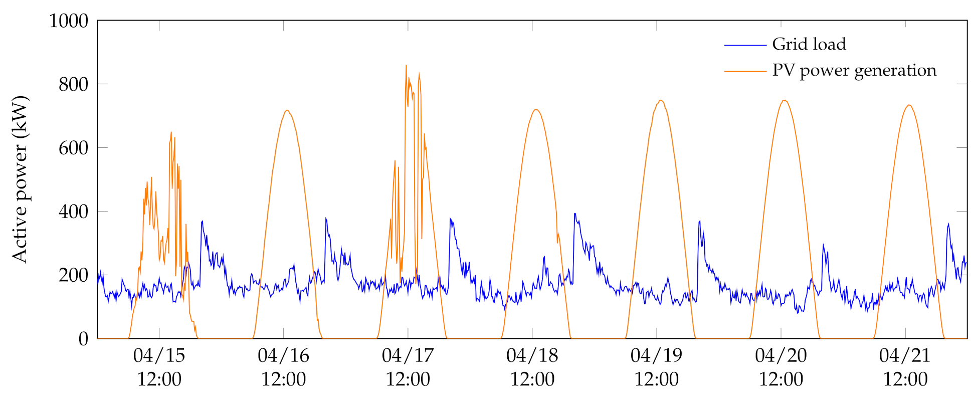
2.3. PV Power Generation Inferred from Global Horizontal Irradiance

PV power generation values are inferred from global horizontal irradiance values using the following Equation [44]:

$${\widehat{\mathit{P}}}_{\mathrm{PV}}\left(t\right)={\eta }_{T_{ref}}·S·\widehat{\mathbf{GHI}}\left(t\right)·{\tau }_{\alpha }\left[1-{\beta }_{ref}\left(T_p-T_{ref}\right)\right]$$

(8)

where ${\eta }_{T_{ref}}$ (herein, ${\eta }_{T_{ref}}=0.21$) is the PV panel’s efficiency, S is the total surface area of PV panels in the power distribution grid, $\widehat{\mathbf{GHI}}$ are global horizontal irradiance forecasts, ${\tau }_{\alpha }$ is the effective transmittance of the PV panels (herein, ${\tau }_{\alpha }=0.95$), ${\beta }_{ref}$ is the coefficient of power degradation due to high temperatures (${\beta }_{ref}=0.004$), $T_{ref}$ is the reference temperature (herein, $T_{ref}=25{}^{\circ }\mathrm{C}$), and $T_p$ is the PV panels’ temperature, computed as follows [45]:

$$T_p\left(t\right)=T_a\left(t\right)+k·\widehat{\mathbf{GHI}}\left(t\right)$$

(9)

where $T_a$ is the ambient temperature and $k=0.025$.

2.4. Initial Operation Strategy

The initial operation of the flexible assets does not take into account power grid regulation purposes [20]. The biogas plant’s power generation is a constant nominal value (herein, $P_{b,n}=100\mathrm{k}\mathrm{W}$). This is in line with the steady biogas flow generated by the bioreactor and coming into the storage unit. As for the water tower, its water pump is subject to an ON/OFF controller, which ensures that the water level remains between two threshold values at all times (herein, $P_{w,n}=100\mathrm{k}\mathrm{W}$). Both assets’ priority is maintaining storage volume levels within pre-fixed extrema, which can sometimes be in conflict with the grid stability’s best interest.

3. Intraday Forecasting of Stochastic Quantities

3.1. Introduction

In the context of the control strategy proposed in this paper, the three stochastic quantities that come into play are the following: power grid load, global horizontal irradiance (GHI) [46,47,48], and water demand. The power grid load represents agglomerated power demand of households in the studied suburban area. It is the grid operator’s priority to make sure this demand is met at all times, under adequate quality and security standards. PV power generation, inferred from GHI values as explained in Section 2.3, represents the agglomerated power generation of household PV panels in the studied area (the residential neighbourhood). One of the assets used by the control strategy is the water tower, whose operational priority is meeting the water demand. In this paper, the methodology used to forecast each of these quantities and its results are briefly presented.

As part of the research activities of the PROMES-CNRS laboratory, a comparative study of models developed for multi-step-ahead GHI forecasting is carried out for intrahour and intraday forecast horizons using a two-year database of GHI measurements sampled at a 10-min rate. Results demonstrate that, although all considered models outperform the persistence model, there is no clear frontrunner in terms of nRMSE values, with a slight advantage for LSTM (long short term memory) artificial neural network (ANN) and Gaussian process regression (GPR) models when taking into account the quality of the forecasts’ associated confidence intervals.

Confidence intervals are a noteworthy perk of using GPR models in the forecast module of the smart management strategy since they are built-in in the models and do not require running a Monte Carlo simulation to be statistically inferred as is the case for other forecasting methods (like artificial neural networks). These confidence intervals give the predictive controller supplementary information it uses to achieve a more robust control strategy. The development of GPR models for intraday GHI forecasting are detailed in [46,47,48].

GPR models used herein are, in part due to the fact that the database used to update the model’s parameters is a sliding one, sufficiently fast to be a valid candidate for the real-time control application at hand. On the downside, the predictive nature of the controller makes it dependant upon real-time access to measurements to be able to sustain the forecasting models’ sliding databases and to update their parameters at each time step. This limitation is true for all machine-learning-based methods operating in real time, hence the growing interest in the development of state-of-the-art smart metering technologies that ensure quick and reliable data transfer.

For the reasons listed above, the choice has been made to develop GPR models to provide intraday forecasts for the smart management scheme developed herein. The associated confidence intervals are incorporated into the control scheme to improve its robustness to forecasting errors as explained in Section 4. This is the main contribution of the paper as it focuses on the developement of a resilient predictive control strategy for low-voltage power distribution grids with prolific distributed generation.

3.2. Gaussian Process Regression

A Gaussian process (GP) can be seen as a collection of random variables, any finite number of which have a joint Gaussian distribution [48,49]. A prior over functions is defined and can then be converted into a posterior over functions once some data has been observed (i.e., observations). $f\left(x\right)\sim \mathcal{GP}(\mu \left(x\right),k(x,x^{\prime }))$, with x and $x^{\prime }$ arbitrary input variables, $\mu \left(x\right)=\mathbb{E}\left[f\left(x\right)\right]$ the mean function (which is usually assumed to be null) and $k(x,x^{\prime })=\mathbb{E}\left[(f\left(x\right)-\mu \left(x\right))(f\left(x^{\prime }\right)-\mu {\left(x^{\prime }\right)}^{\mathsf{T}})\right]$ the covariance function (also known as kernel), indicates that this random function follows a GP. The interested reader is referred to [49] for a detailed explanation of Gaussian processes and Gaussian process regression (GPR).

The standard regression model with additive noise is formulated as follows:

$$\begin{array}{c}\hfill y=f\left(x\right)+\epsilon \end{array}$$

(10)

where $x\in {\mathbb{R}}^{D\times 1}$ is the input vector with a dimension of 1, f is the regression function, y is the observed value and $\epsilon \sim \mathcal{N}(0,{\sigma }_{\epsilon }^2)$ is an independent, identically distributed Gaussian noise.

The mean prediction ${\mu }_{\ast }$ can be written as a linear combination of kernel functions, each one centred on a data point:

$$\begin{array}{c}\hfill {\mu }_{\ast }=\mu \left(x_{\ast }\right)+k_{\ast }^{\mathsf{T}}·\alpha =\mu \left(x_{\ast }\right)+\sum _{i=1}^n{\alpha }_i·k(x_i,x_{\ast })\end{array}$$

(11)

where $\alpha ={\left(K+{\sigma }_{\epsilon }^2·I\right)}^{-1}(y-\mu \left(x_{\ast }\right))$. The coefficients ${\alpha }_i$ are referred to as parameters.

It is possible to combine several kernel functions to obtain a more complex one. The only requirement is that the resulting covariance matrix must be a positive semi-definite function. A detailed list of kernel functions is provided in [49]. Hereinafter, the kernel functions used in this work are defined.

The periodic kernel (Per) is given by:

$$k_{\mathrm{Per}}(x,x^{\prime })={\sigma }_1^2·exp\left(-\frac{2{sin}^2\left(\frac{\pi (x-x^{\prime })}{P}\right)}{{\ell }_1^2}\right)$$

(12)

where ${\sigma }_1$ is the amplitude, ${\ell }_1$ is the correlation length and P is the period.

The isotropic squared exponential (SE) kernel is given by:

$$k_{\mathrm{SE}}(x,x^{\prime })={\sigma }_2^2·exp\left(-\frac{{(x-x^{\prime })}^2}{2{\ell }_2^2}\right)$$

(13)

where ${\sigma }_2$ is the amplitude and ${\ell }_2$ is the correlation length.

The isotropic rational quadratic (RQ) kernel is given by:

$$k_{\mathrm{RQ}}(x,x^{\prime })={\sigma }_3^2{\left(1+\frac{{(x-x^{\prime })}^2}{2{\ell }_3^2·\alpha }\right)}^{-\alpha }$$

(14)

where ${\sigma }_3$ is the amplitude, ${\ell }_3$ is the correlation length and $\alpha$ defines the relative weighting of large-scale and small-scale variations.

In addition to forecasts, the regression model provides an associated confidence interval within which measurements have a probability of 95% of staying. This interval ($\mathbb{CI}$) is computed as follows:

$$\mathbb{CI}={\mu }_{\ast }\pm 1.96\sqrt{{\sigma }_{\ast }^2}$$

(15)

where $\mathbb{CI}$ represent the confidence interval bounds, ${\mu }_{\ast }$ is the predictive mean, and ${\sigma }_{\ast }$ is the predictive variance.

During the training phase, the values of hyperparameters are optimised using a 2-week database [48]. During the test phase, at every time step, new measurements are incorporated in order to update values of the model’s parameters using a sliding 24 h database.

3.3. Data Description and Kernel Compositions

The forecast horizons considered in this work are intraday: they range from 1 h to 24 h. For the training phase, two weeks of data are used. The testing phase is then performed over one week. Available data of power grid load, water demand, and global horizontal irradiance span a year for the three stochastic quantities. They are sampled at a 10-min rate. An examination of the signals’ behaviours informs the following choices of kernel compositions for their intraday forecasting.

• Power grid load

  $$k^{gl}(x,x^{\prime })=k_{\mathrm{Per}}^{gl}(x,x^{\prime })+k_{\mathrm{SE}}^{gl}(x,x^{\prime })+k_{\mathrm{RQ}}^{gl}(x,x^{\prime })$$

  (16)
  Herein, the period of the data is 24 h and the structure of $k_{\mathrm{Per}}^{gl}$ translates the daily periodic pattern. $k_{\mathrm{SE}}^{gl}$ is used to capture the long-term trend of the data, namely the seasonal tendencies present in the power grid load. $k_{\mathrm{RQ}}^{gl}$ is used to capture the intraday variations observed in the data, namely intraday fluctuations due to behavioural patterns of end-users.
• Water demand

  $$k^{wt}(x,x^{\prime })=k_{\mathrm{Per}}^{wt}(x,x^{\prime })+k_{\mathrm{SE}}^{wt}(x,x^{\prime })$$

  (17)
  $k_{\mathrm{Per}}^{wt}$ models the daily periodic shape of the data and $k_{\mathrm{SE}}^{wt}$ is used to fit the data’s intraday fluctuations. A brief kernel study leads to the conclusion that the simple addition of a squared exponential kernel is sufficient to have satisfactory results without adding too much computational burden to the model.
• Global horizontal irradiance

  $$k^{\mathrm{GHI}}(x,x^{\prime })=k_{\mathrm{Per}}^{\mathrm{GHI}}(x,x^{\prime })·k_{\mathrm{RQ}}^{\mathrm{GHI}}(x,x^{\prime })$$

  (18)
  $k_{\mathrm{Per}}^{\mathrm{GHI}}$ models the daily periodic shape of the data and $k_{\mathrm{RQ}}^{\mathrm{GHI}}$ captures the intraday fluctuations present in these data. A thorough study has been conducted in [47] to determine the most suitable kernel composition for intraday GHI forecasting.

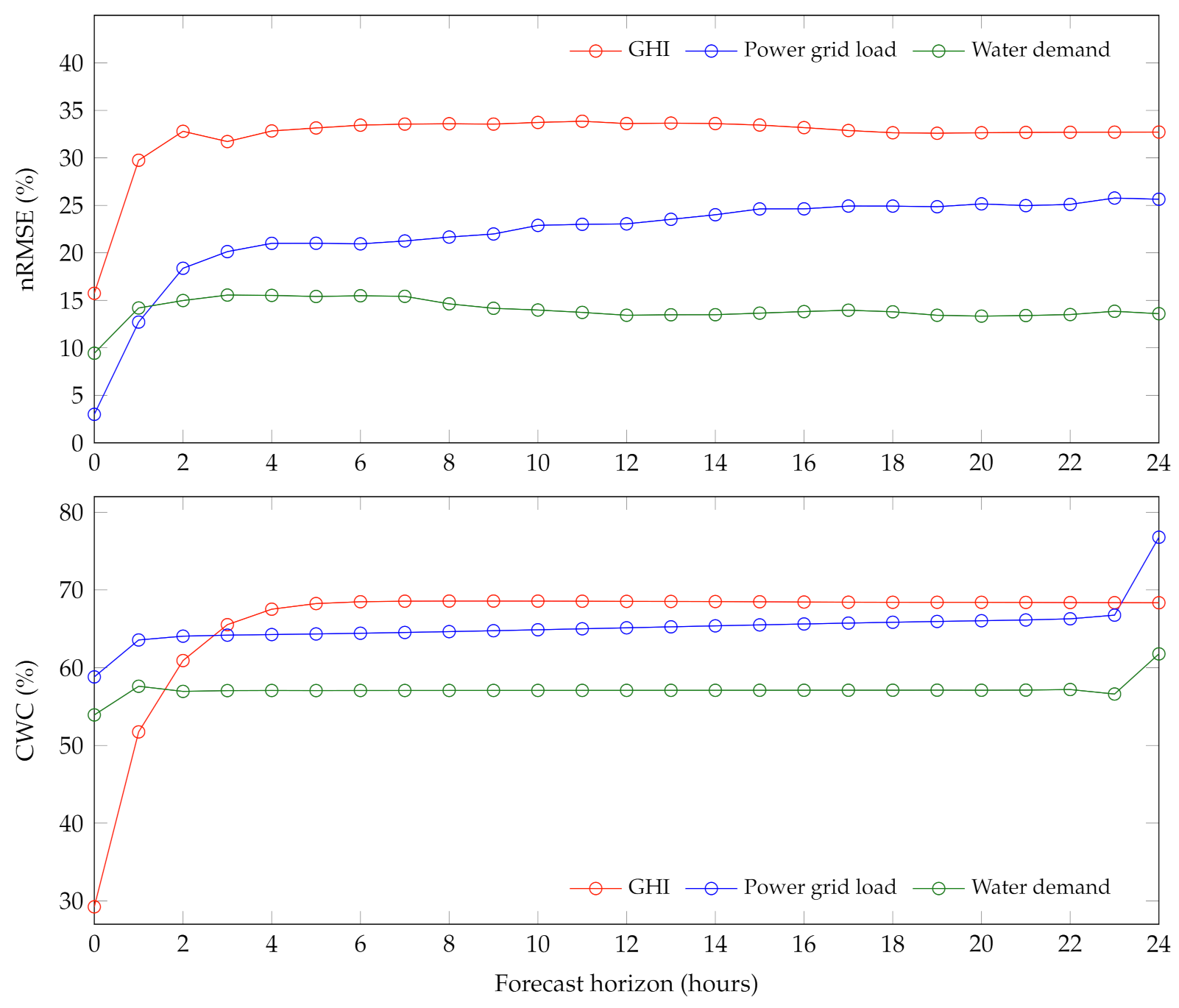
3.4. Forecasting Results

The evaluation metrics used in this work, evaluated over the considered week in April (see Figure 1), are the following:

• The normalized root mean square error (nRMSE), expressed as follows:

  $$\mathrm{nRMSE}=100\frac{\sqrt{\frac{1}{n_{\ast }}{\sum }_{i=1}^{n_{\ast }}{\left(y_{\mathrm{test}}\left(i\right)-y_{\mathrm{forecast}}\left(i\right)\right)}^2}}{\frac{1}{n_{\ast }}{\sum }_{i=1}^{n_{\ast }}{y}_{\mathrm{test}}\left(i\right)}$$

  (19)

  where $y_{\mathrm{test}}\in {\mathbb{R}}^{n_{\ast }\times 1}$ are the test data, $y_{\mathrm{forecast}}\in {\mathbb{R}}^{n_{\ast }\times 1}$ are the forecasts given by the models, and $n_{\ast }$ is the number of data points in the forecast horizon.
• The coverage width-based criterion ($\mathrm{CWC}$) [50], defined as a combination of two different criteria, i.e., the prediction interval normalized average width ($\mathrm{PINAW}$) and the prediction interval coverage probability ($\mathrm{PICP}$).
  The $\mathrm{PINAW}$ criterion allows the surface area of the confidence intervals associated with the forecasts to be assessed:

  $$\mathrm{PINAW}=\frac{1}{n·R}\sum _{i=1}^n(U_i-L_i)$$

  (20)

  where R is the difference between the maximum and minimum in test data and $U_i$ and $L_i$ are the upper and lower bounds of the confidence interval, respectively.
  The $\mathrm{PICP}$ criterion informs on the probability that measurements would fall within the confidence interval:

  $$\mathrm{PICP}=\frac{1}{n}\sum _{i=1}^n{ϵ}_i$$

  (21)

  where ${ϵ}_i$ is used to detect whether the target value is in the confidence interval.
  The coverage width-based criterion ($\mathrm{CWC}$) is then defined as follows:

  $$\mathrm{CWC}=\mathrm{PINAW}\left(1+\gamma \left(\mathrm{PICP}\right)·exp(-\eta ·(\mathrm{PICP}-\mu \left)\right)\right)$$

  (22)

  where $\eta$ ($\eta =10$) and $\mu$ ($\mu =0.95$) are parameters, and $\gamma$ is defined such that:

  $$\gamma \left(x\right)=\left\{\begin{array}{cc}1\hfill & \mathrm{if}x<\mu \hfill \\ 0\hfill & \mathrm{if}x⩾\mu \hfill \end{array}\right.$$

  (23)

Figure 2 displays nRMSE values of intraday forecasts of power grid load, water demand, and GHI. For intraday forecasts of grid load, results show that the GPR model performs well for short time horizons. However, the forecasting error rapidly increases as the forecast horizon does, which is an expected result. For a 1-h horizon, the GPR model achieves an error as low as 13%. As for the 6-h horizon and the 12-h one, nRMSE values are virtually constant (21% and 23%, respectively). This remains the case for a forecast horizon of 24 h, where the GPR model has an error of 26%.

For intraday forecasts of water demand, values of nRMSE start at 9% for a 10 min forecast and quickly stabilises around 13% for longer forecast horizons. Due to the data’s regular nature, a simple combination of a periodic kernel and a rational quadratic kernel for intraday fluctuations proves enough to capture the data’s behaviour quite faithfully. As for intraday forecasts of GHI (from which PV power generation is inferred), the selected GPR model performs well for short forecast horizons (15.74% for a 10-min forecast horizon), but its performance degrades as the forecast horizon grows and it stabilises around 32% for horizons beyond 6 h. This is reflected in the temporal evolution of the forecasts, where it can be seen that intraday fluctuations become increasingly difficult to fit. Further work is currently underway to enhance the model’s performance for long intraday forecast horizons.

Figure 2 also displays values of $\mathrm{CWC}$, which follow similar patterns to those of nRMSE values: starting with lower values for short forecast horizons, then quickly stabilizing around a constant value for longer horizons. It can be seen that the higher the nRMSE values, the higher the corresponding $\mathrm{CWC}$ values. They stabilize around 57% for water demand forecasts, around 65% for grid load forecasts, and around 68% for GHI forecasts.

4. Model-Based Predictive Control Strategy

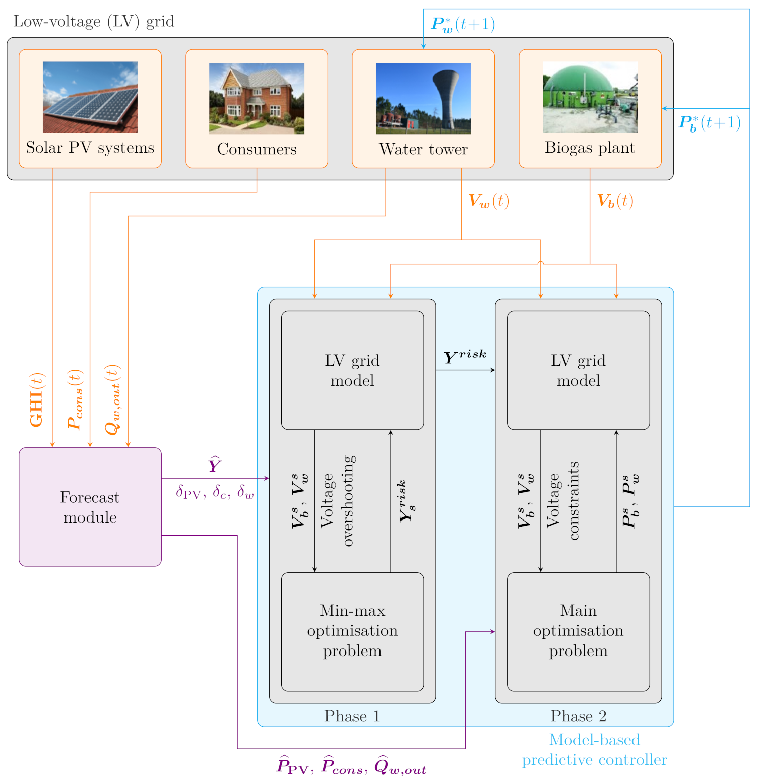
4.1. Inner-Workings of the Smart Management Scheme

Figure 3 shows the synoptic scheme of the proposed MPC strategy. The following is a detailed explanation of the different steps taken by the proposed strategy at each time step.

• Data acquisition: measurements are taken of stored biogas volume and stored water volume and are injected into the predictive controller in order to update the system’s state. GHI and grid load are measured and water demand is inferred from measurements of water volume and incoming flow rate ${\mathit{Q}}_{\mathit{w},\mathit{in}}$. These values are injected into the forecast module.
• Forecast module: measured values of the controller’s stochastic inputs (GHI, grid load, and water demand inferred from incoming flow rate) are added to the sliding databases of respective GPR models, which are then used to update the models’ parameters. Afterwards, the module produces updated forecasts of all three stochastic quantities over the forecast horizon, along with their respective confidence intervals. Lastly, GHI values and their corresponding confidence intervals are converted into PV power generation ones.
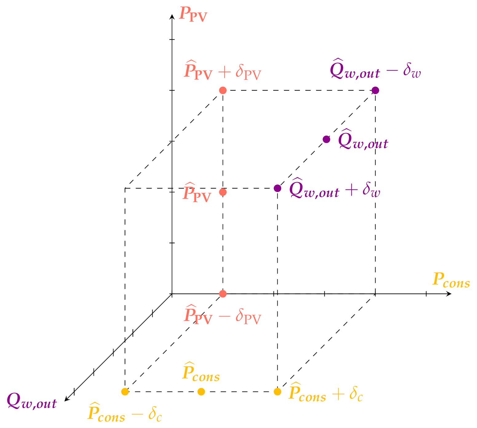
• Worst-case scenario: phase 1 of the controller’s decision-making process consists in determining the stochastic input values corresponding to the worst-case scenario of the following time slot, in terms of constraint violation. This bloc receives measurements of biogas volume and water volume, GPR forecasts of PV power generation, grid load, and water demand for the following time slot, and confidence intervals of GPR forecasts for the following time slot.
  An optimisation algorithm searches the feasible space defined in Figure 4 for worst-case scenario input values. It does so based on the optimisation problem formulated by Equations (46)–(49) and using the low-voltage grid model to evaluate volume bounds and potential voltage overshooting.
• Reduction of power supply/demand unbalance: phase 2 of the controller’s decision-making process consists in determining the flexible assets’ optimal setpoints. This bloc receives GPR forecasts of PV power generation, grid load, and water demand over the entire forecast horizon, as well as worst-case scenario input values of the following time slot, produced by phase 1.
  An optimisation algorithm searches for optimal setpoints of biogas plant power generation and water tower power consumption. It does so based on the optimisation problem defined in Section 4.2 and using the low-voltage grid model based on Kirchhoff laws to evaluate various constraints.
• Implementation of flexible assets’ setpoints: optimal setpoints of flexible assets are produced, the first step of which are implemented by the biogas plant and the water tower.

4.2. Main Optimisation Problem

The optimisation problem [20] is formulated such as the discrete setpoint values of the water tower are replaced with a real-values optimisation variable $\overline{\mathit{t}}\in {\mathbb{R}}^{H_p}$, with $H_p$ the integer number of time slots within the forecast horizon, effectively avoiding the MINLP setting [28,29,30,31,32,33,34] without relaxing the problem. In fact, between sampling times $t_i$ and $t_{i+1}$, the water tower can switch between its two states of operation ($P_{w,min}$ and $P_{w,max}$) and the biogas plant can switch between two setpoints within the interval $[P_{b,min},P_{b,max}]$. If the assets do make the switch within a given time slot, they do so at the same instant ${\overline{t}}_i$. Let us denote $\mathit{X}$ as follows:

$$\mathit{X}={\left[\begin{array}{c}{\mathit{P}}_{\mathit{b},\mathbf{ON}}{\mathit{P}}_{\mathit{b},\mathbf{OFF}}\overline{\mathit{t}}{\mathit{U}}_{\mathbf{ON},q}{\mathit{U}}_{\mathbf{OFF},q}\end{array}\right]}^{\mathsf{T}}$$

(24)

where ${\mathit{P}}_{\mathit{b},\mathbf{ON}}\in {\mathbb{R}}^{H_p}$ and ${\mathit{P}}_{\mathit{b},\mathbf{OFF}}\in {\mathbb{R}}^{H_p}$ form the biogas plant setpoint like this:

$${\mathit{P}}_{\mathit{b}}\left(\tau \right)=\left\{\begin{array}{c}{\mathit{P}}_{\mathit{b},\mathbf{ON}}\left(\tau \right),\tau \in [t_i,t_i+{\overline{t}}_i]\hfill \\ {\mathit{P}}_{\mathit{b},\mathbf{OFF}}\left(\tau \right),\tau \in [t_i+{\overline{t}}_i,t_{i+1}]\hfill \end{array}\right.$$

(25)

For every node $q\in \{1,\dots ,N\}$, ${\mathit{U}}_{\mathbf{ON},q}\in {\mathbb{R}}^{(H_p·N)}$ and ${\mathit{U}}_{\mathbf{OFF},q}\in {\mathbb{R}}^{(H_p·N)}$ form the voltages in the grid:

$${\mathit{U}}_q\left(\tau \right)=\left\{\begin{array}{c}{\mathit{U}}_{\mathbf{ON},q}\left(\tau \right),\tau \in [t_i,t_i+{\overline{t}}_i]\hfill \\ {\mathit{U}}_{\mathbf{OFF},q}\left(\tau \right),\tau \in [t_i+{\overline{t}}_i,t_{i+1}]\hfill \end{array}\right.$$

(26)

The optimisation problem can be solved at each time step assuming that the first state of the water tower is always ON. In some extreme cases, this assumption may induce some issues of implementability given volume constraints, which are tackled in a post-treatment phase (the interested reader is referred to [20] for details about the post-treatment algorithm). However, this simplification reduces the complexity of the model without sacrificing much performance. The objective function $f_{obj}$ is formulated as follows:

$$f_{obj}\left(\mathit{X}\right)=\sum _{i=0}^{H_p-1}\left[\underset{t_i}{\overset{t_i+{\overline{t}}_i}{\int }}{\mathit{S}}_{\mathbf{ON}}\left(\tau \right)\mathrm{d}t+\underset{t_i+{\overline{t}}_i}{\overset{t_{i+1}}{\int }}{\mathit{S}}_{\mathbf{OFF}}\left(\tau \right)\mathrm{d}t\right]$$

(27)

with

$$\begin{array}{c}{\mathit{S}}_{\mathbf{ON}}\left(\tau \right)={|{\mathit{P}}_{\mathrm{PV}}\left(\tau \right)+{\mathit{P}}_{\mathit{b}}\left(\tau \right)-{\mathit{P}}_{\mathit{cons}}\left(\tau \right)-P_{w,max}|}^2\end{array}$$

(28)

$$\begin{array}{c}{\mathit{S}}_{\mathbf{OFF}}\left(\tau \right)={|{\mathit{P}}_{\mathrm{PV}}\left(\tau \right)+{\mathit{P}}_{\mathit{b}}\left(\tau \right)-{\mathit{P}}_{\mathit{cons}}\left(\tau \right)-P_{w,min}|}^2\end{array}$$

(29)

The optimisation problem is then formulated as follows:

$${\mathit{X}}^{\ast }=arg\underset{\mathit{X}}{min}{f}_{obj}\left(\mathit{X}\right)$$

(30)

and is subject to the following bounds and constraints, $\forall i\in \{1,\dots ,H_p\}$:

• Biogas plant power bounds

  $$\begin{array}{c}{P}_{b,min}⩽{\mathit{P}}_{\mathit{b},\mathbf{ON}}\left(\tau \right)⩽P_{b,max}\end{array}$$

  (31)

  $$\begin{array}{c}{P}_{b,min}⩽{\mathit{P}}_{\mathit{b},\mathbf{OFF}}\left(\tau \right)⩽P_{b,max}\end{array}$$

  (32)
• Switch time bounds

  $$\begin{array}{c}0⩽{\overline{t}}_i⩽T\end{array}$$

  (33)
• Biogas volume constraints

  $$\begin{array}{c}{V}_{b,min}⩽{\mathit{V}}_{\mathit{b}}\left(t\right)⩽V_{b,max}\end{array}$$

  (34)
• Water volume constraints

  $$\begin{array}{c}{V}_{w,min}⩽{\mathit{V}}_{\mathit{w}}\left(t\right)⩽V_{w,max}\end{array}$$

  (35)
• Voltage constraints

  $$\begin{array}{c}{\overline{t}}_i·K_t({\mathit{P}}_{\mathit{b},\mathbf{ON}}\left(\tau \right),P_{w,max},{\mathit{U}}_{\mathbf{ON},q}\left(\tau \right))=0\end{array}$$

  (36)

  $$\begin{array}{c}(T-{\overline{t}}_i)·K_t({\mathit{P}}_{\mathit{b},\mathbf{OFF}}\left(\tau \right),P_{w,min},{\mathit{U}}_{\mathbf{OFF},q}\left(\tau \right))=0\end{array}$$

  (37)

  $$\begin{array}{c}|{\mathit{U}}_{\mathbf{ON},q}\left(\tau \right)-U_n|⩽\delta U\end{array}$$

  (38)

  $$\begin{array}{c}|{\mathit{U}}_{\mathbf{OFF},q}\left(\tau \right)-U_n|⩽\delta U\end{array}$$

  (39)

$K_t$ describes voltage variations across the low-voltage power distribution grid as a function of the power which is injected or absorbed at each node. Kirchhoff’s law constraints are presented as two sets of constraints (Equations (36) and (37)), which guarantee that Kirchhoff’s laws are upheld in both sub-intervals of each time slot. The equation set depicting voltage variations is multiplied by ${\overline{t}}_i$ (Equation (36)) or $T-{\overline{t}}_i$ (37), using appropriate values of biogas plant and water tower setpoints for each interval, in order to ensure that only one constraint is activated in case of extreme values of ${\overline{t}}_i$. In fact, in case ${\overline{t}}_i=0$, Equation (36) is ignored, reflecting the fact that during time slot i, the water tower is turned off immediately at the beginning of the time slot. Likewise, in case ${\overline{t}}_i=T$, Equation (37) is ignored since the water tower remains on for the duration of the time slot. Voltage constraints are also written as two sets of constraints (Equations (38) and (39)) that account for voltage variations in both states of the low-voltage power distribution grid within each time slot. While depicting the same physical constraints, this problem formulation has a bigger feasible set than the MINLP one [28,29,30,31,32,33,34]. As a result, with such a formulation, the global optimum is guaranteed to be equal or better than the one of the MINLP formulation.

4.3. The Worst-Case Scenario Approach

In this section, amendments are made to the predictive control strategy in order to enhance the controller’s performance by making it more robust to forecasting errors of the system’s various stochastic quantities. The premise of the method is to use min–max optimisation in order to find and solve a “worst-case scenario" at each time step based on confidence intervals given by the inputs’ respective GPR models. Eliminating, or at least minimising, the constraint violations corresponding to the worst-case scenario guarantee that these violations are also minimised for all other possible scenarios.

It should be noted that, at each time step, these amendments are only made to the decision-making of the subsequent time step, and not over the entire forecast horizon. This choice is motivated by two reasons. The first is that determining a worst-case scenario over the entire forecast horizon is a conservative and computationally expensive optimisation problem, which is incompatible with the real-time application at hand. As a matter of fact, a min–max problem over the entire forecast horizon has a feasible space of dimension $(3\times H_p)$, as opposed to the problem concerned only with the following time step only having a 3-dimensional feasible space. The second is that, due to the closed-loop nature of MPC, computing robust setpoints for the entire forecast horizon is in high likelihood a waste of resources because, at each time step, only the first setpoint is applied and the whole procedure is reiterated at the next one. Ergo, the scheme only seeks to provide a setpoint robust to forecasting errors for the next time step.

First, let ${\widehat{\mathit{P}}}_{\mathbf{PV}}$, ${\widehat{\mathit{P}}}_{\mathit{cons}}$, and ${\widehat{\mathit{Q}}}_{\mathit{w},\mathit{out}}$ be forecasted values of PV power generation, grid load, and water demand, respectively, over the forecast horizon. Then, let ${\mathit{P}}_{\mathbf{PV}}$, ${\mathit{P}}_{\mathit{cons}}$, and ${\mathit{Q}}_{\mathit{w},\mathit{out}}$ be measured values of PV power generation, grid load, and water demand, respectively, over the forecast horizon. Finally, ${\delta }_{\mathrm{PV}}$, ${\delta }_c$, and ${\delta }_w$ define confidence intervals, for the next time step, of GPR forecasts of PV power generation, grid load, and water demand, respectively, as follows:

$$\begin{array}{c}{\mathit{P}}_{\mathbf{PV}}(t+1)\in [{\widehat{\mathit{P}}}_{\mathbf{PV}}(t+1)-{\delta }_{\mathrm{PV}},{\widehat{\mathit{P}}}_{\mathbf{PV}}(t+1)+{\delta }_{\mathrm{PV}}]\end{array}$$

(40)

$$\begin{array}{c}{\mathit{P}}_{\mathit{cons}}(t+1)\in [{\widehat{\mathit{P}}}_{\mathit{cons}}(t+1)-{\delta }_c,{\widehat{\mathit{P}}}_{\mathit{cons}}(t+1)+{\delta }_c]\end{array}$$

(41)

$$\begin{array}{c}{\mathit{Q}}_{\mathit{w},\mathit{out}}(t+1)\in [{\widehat{\mathit{Q}}}_{\mathit{w},\mathit{out}}(t+1)-{\delta }_w,{\widehat{\mathit{Q}}}_{\mathit{w},\mathit{out}}(t+1)+{\delta }_w]\end{array}$$

(42)

Herein, the confidence intervals are computed such that there is a 95% probability of measurements remaining inside them (15). There exists a triplet $({\mathit{P}}_{\mathbf{PV}}^{\mathit{risk}}(t+1),{\mathit{P}}_{\mathit{cons}}^{\mathit{risk}}(t+1),{\mathit{Q}}_{\mathit{w},\mathit{out}}^{\mathit{risk}}(t+1))$, contained in the feasible space illustrated in Figure 4, that induces a worst-case scenario vis-a-vis the optimisation problem constraints in the next time step. Finding this triplet and incorporating it into the predictive control strategy described in Section 4 allows the controller to adjust its decision-making in order to reduce, if possible eliminate, any constraint violation that could occur in the next time step as a result of the stochastic quantities’ measured values being different from the forecasted ones, within the limits of the associated confidence intervals. Let $\mathit{Y}$ be the vector containing measurements of PV power generation, grid load, and water demand, for the next time step:

$$\mathit{Y}={\left[\begin{array}{c}{\mathit{P}}_{\mathbf{PV}}(t+1){\mathit{P}}_{\mathit{cons}}(t+1){\mathit{Q}}_{\mathit{w},\mathit{out}}(t+1)\end{array}\right]}^T$$

(43)

Let $\widehat{\mathit{Y}}$ be the vector containing forecasts of PV power generation, grid load, and water demand, for the next time step:

$$\widehat{\mathit{Y}}={\left[\begin{array}{c}{\widehat{\mathit{P}}}_{\mathbf{PV}}(t+1){\widehat{\mathit{P}}}_{\mathit{cons}}(t+1){\widehat{\mathit{Q}}}_{\mathit{w},\mathit{out}}(t+1)\end{array}\right]}^T$$

(44)

Let ${\mathit{Y}}^{\mathit{risk}}$ be the vector comprised of critical values defining the worst-case scenario of the next time step:

$${\mathit{Y}}^{\mathit{risk}}={\left[{\mathit{P}}_{\mathbf{PV}}^{\mathit{risk}}(t+1){\mathit{P}}_{\mathit{cons}}^{\mathit{risk}}(t+1){\mathit{Q}}_{\mathit{w},\mathit{out}}^{\mathit{risk}}(t+1)\right]}^T$$

(45)

where ${\mathit{P}}_{\mathbf{PV}}^{\mathit{risk}}$, ${\mathit{P}}_{\mathit{cons}}^{\mathit{risk}}$, and ${\mathit{Q}}_{\mathit{w},\mathit{out}}^{\mathit{risk}}$ are critical values of PV power generation, grid load, and water demand, respectively, corresponding to the worst-case scenario.

Based on Equations (40)–(42), ${\mathit{Y}}^{\mathit{risk}}$ exists in the feasible space illustrated by Figure 4. At every time step, the following min–max problem is solved:

$${\mathit{Y}}^{\mathit{risk}}=arg\underset{\mathit{Y}}{min}\left(-\Phi \left(\mathit{Y}\right)\right)$$

(46)

where $\Phi \left(\mathit{Y}\right)$ is the voltage undershooting/overshooting corresponding to input values of $\mathit{Y}$, as defined in Section 5.1, subject to:

$$\begin{array}{c}\widehat{\mathit{Y}}\left(1\right)-{\delta }_{\mathrm{PV}}⩽\mathit{Y}\left(1\right)⩽\widehat{\mathit{Y}}\left(1\right)+{\delta }_{\mathrm{PV}}\end{array}$$

(47)

$$\begin{array}{c}\widehat{\mathit{Y}}\left(2\right)-{\delta }_c⩽\mathit{Y}\left(2\right)⩽\widehat{\mathit{Y}}\left(2\right)+{\delta }_c\end{array}$$

(48)

$$\begin{array}{c}\widehat{\mathit{Y}}\left(3\right)-{\delta }_w⩽\mathit{Y}\left(3\right)⩽\widehat{\mathit{Y}}\left(3\right)+{\delta }_w\end{array}$$

(49)

5. Results and Analysis

5.1. Evaluation Metrics

Various evaluation metrics used throughout this paper are defined hereinafter. Let $H_t$ be the number of time slots in the simulation period.

• Final value of the objective function: its square root ($\sqrt{f_{obj,final}}$) represents the cumulative gap between power supply and demand within the power distribution grid during the simulated week.
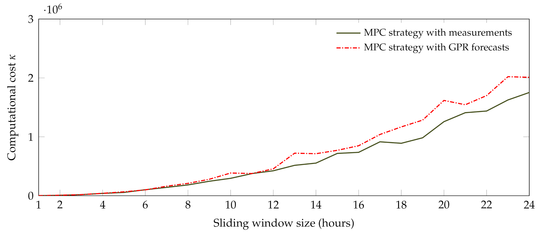
• Computational complexity $\kappa$: it is quantified by the mean number of objective function evaluations per window, weighted by its size. The number of objective function evaluations is provided as an output argument of the optimisation function “fmincon” in Matlab.
• Mean deviation from the forecasted values: let ${\overline{\mathit{P}}}_{\mathbf{PV}}$, ${\overline{\mathit{P}}}_{\mathit{cons}}$, and ${\overline{\mathit{Q}}}_{\mathit{w},\mathit{out}}$ be vectors grouping one-step-ahead forecasts (herein, 10-min forecasts) of PV power generation, grid load, and water demand, respectively, during the simulation period. This evaluation metric represents the mean deviation of stochastic input values from the ones forecasted at a one-step-ahead forecast horizon. ${\Omega }_{P_{\mathrm{PV}}}$, which is the mean deviation of PV power generation values (${\mathit{P}}_{\mathbf{PV}}$) from the ones forecasted at a one-step-ahead forecast horizon (in $\mathrm{W}$), is given by:

  $${\Omega }_{P_{\mathrm{PV}}}=\frac{{\sum }_{t=0}^{H_t-1}{\overline{\mathit{P}}}_{\mathbf{PV}}(t+1)-{\mathit{P}}_{\mathbf{PV}}(t+1)}{H_t}$$

  (50)
  ${\Omega }_{P_{cons}}$, which is the mean deviation of grid load values (${\mathit{P}}_{\mathit{cons}}$) from the ones forecasted at a one-step-ahead forecast horizon (in $\mathrm{W}$), is given by:

  $${\Omega }_{P_{cons}}=\frac{{\sum }_{t=0}^{H_t-1}{\overline{\mathit{P}}}_{\mathit{cons}}(t+1)-{\mathit{P}}_{\mathit{cons}}(t+1)}{H_t}$$

  (51)
  ${\Omega }_{Q_{w,out}}$, which is the mean deviation of water demand values (${\mathit{Q}}_{\mathit{w},\mathit{out}}$) from the ones forecasted at a one-step-ahead forecast horizon (in ${\mathrm{m}}^3{\mathrm{h}}^{-1}$), is given by:

  $${\Omega }_{Q_{w,out}}=\frac{{\sum }_{t=0}^{H_t-1}{\overline{\mathit{Q}}}_{\mathit{w},\mathit{out}}(t+1)-{\mathit{Q}}_{\mathit{w},\mathit{out}}(t+1)}{H_t}$$

  (52)
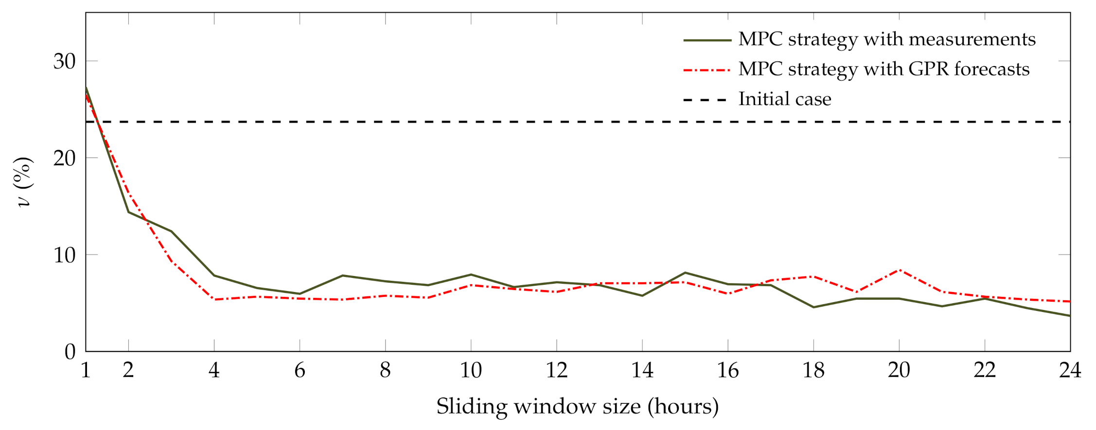
• Instances of voltage overshooting $\nu$: in cases where the main optimisation problem has no feasible solution, overvoltage or undervoltage may occur in the power distribution grid. These are the instances that the present paper studies and attempts to reduce. This metric records the percentage of these instances during the simulation period.
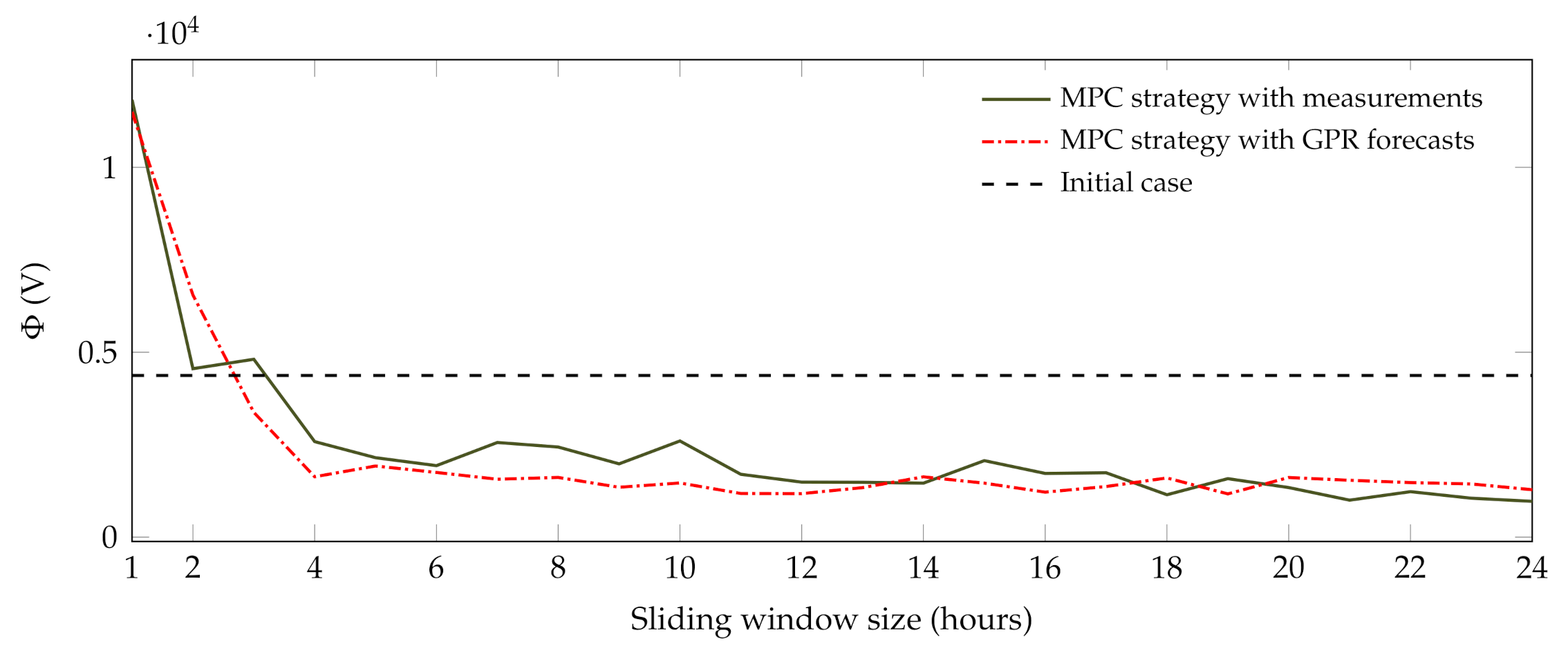
• Surface area of voltage overshooting $\Phi$: this metric is complementary to the number of instances of voltage constraint violation. It represents the total surface area of voltage overshooting past the prescribed lower and upper voltage levels in the power distribution grid, during the simulated period. It is measured in volts and is calculated as follows:

  $$\Phi \left(\mathit{Y}\right)=\sum _{s=1}^N\left(\sum _{t=1}^{H_t}max\left({\mathit{U}}_{\mathit{s}}\left(t\right)-U_{min},U_{max}-{\mathit{U}}_{\mathit{s}}\left(t\right),0\right)\right)$$

  (53)

  where N is the number of nodes in the power distribution grid, $U_{min}$ is the lower voltage threshold, $U_{max}$ is the upper voltage threshold, and ${\mathit{U}}_{\mathit{s}}$, where $s\in \{1,\dots ,N\}$, are voltage values in various nodes of the power distribution grid. Let $\Psi \in {\mathbb{R}}^{H_p\times 3}$ be the matrix containing the measured stochastic inputs of the control strategy, over the simulation period, defined as follows:

  $$\Psi =\left[\begin{array}{c}{\mathit{P}}_{\mathbf{PV}}{\mathit{P}}_{\mathit{cons}}{\mathit{Q}}_{\mathit{w},\mathit{out}}\end{array}\right]$$

  (54)
  Note that voltage values across the power distribution grid are linked to the values of $\Psi$ through Kirchhoff laws.
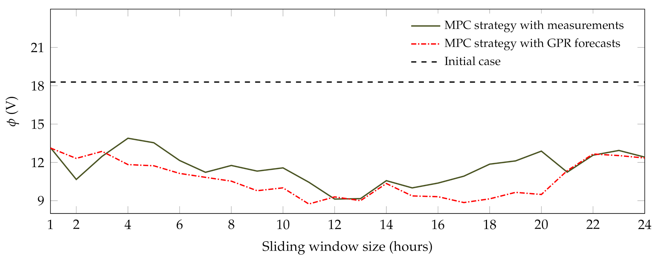
• Average voltage overshooting per time step $\varphi$: it corresponds to the mean of maximum voltage overshooting over the number of instances at which overshooting is observed during the simulation period. It is defined as follows:

  $$\varphi \left(\mathit{Y}\right)=100\frac{{\Phi }_{max}\left(\mathit{Y}\right)}{\nu ·H_t}$$

  (55)

  with

  $${\Phi }_{max}\left(\mathit{Y}\right)=\sum _{t=1}^{H_t}\underset{s\in \{1,\dots ,N\}}{max}\left({\mathit{U}}_{\mathit{s}}\left(t\right)\right)$$

  (56)

  where values of $\mathit{Y}$ and ${\mathit{U}}_{\mathit{s}}$ are related through Kirchhoff laws.

5.2. Impact of Forecasting Errors on MPC Performance

In this section, the impact of forecasting errors on the MPC strategy’s performance is studied. The control scheme is tested over the week in April presented in the previous section and for sliding window sizes ranging from 1 to 24 h. Intraday GPR forecasts of grid load, water demand, and PV power generation (inferred from GHI forecasts), acquired as explained in Section 3, are used to run these simulations.

The performance of the predictive controller fed with GPR forecasts is evaluated in comparison with a controller fed with measurements, i.e., a case where no forecasting errors are made. This comparison will focus on three main aspects of the scheme’s performance: the power supply/demand gap $\sqrt{f_{obj,,final}}$ (Figure 5), computational cost $\kappa$ (Figure 6), and surface area of voltage overshooting $\Phi$ (Figure 7).

In Figure 5, the cumulative power supply/demand gap given by the MPC scheme over the considered week is displayed per sliding window size. Though these values degrade as the sliding window size increases in both cases, the ones given by the MPC scheme when it uses GPR forecasts are not significantly degraded with respect to those given by the MPC scheme that uses measurements. In fact, the maximum difference between the two curves is $198.39$ $\mathrm{k}$$\mathrm{W}$, obtained for the 22-h sliding window, which constitutes only 1.98% of the initial value (10,035 $\mathrm{k}$$\mathrm{W}$).

The computational cost, presented in Figure 6, steadily grows in both cases as the sliding window size does. It is different for the scheme that uses GPR forecasts, which is to be expected since the updated forecasts displace the optimisation problem’s starting point with respect to the previous time step. That being said, the increase in computational cost due to the use of forecasts remains subdued. For window sizes between 1 and 10 h, its average value is a 12.3% increase from the scheme using measurements. For all window sizes up to 24 h, this average is evaluated at 16.4%.

Figure 7 displays the surface area of voltage overshooting, the initial value of which is $4371.4$ $\mathrm{k}$$\mathrm{V}$. For sliding window sizes up to 3 h, the MPC scheme is unable to reduce voltage overshooting and actually makes matters considerably worse. Starting from a 4-h sliding window, voltage overshooting given by the MPC scheme decreases significantly from the initial value, in both the case where the scheme uses measurements and the one where it uses GPR forecasts. Then, for larger window sizes, it quickly stabilizes around the same level. As of the 4 h window size, the MPC strategy effectively eliminates more than 50% of voltage overshooting.

When taking into account the fact that the forecasting errors are at their lowest for short forecast horizons (inferior to 3 h) and rapidly grow for longer horizons, it becomes apparent that the accuracy of forecasts for these short horizons is not enough to guarantee better management of voltage fluctuations on its own. In reality, the availability of forecasts over a longer forecast horizon is pivotal to better equip the MPC scheme to anticipate emerging voltage overshooting and work to prevent it. In light of this observation, it is recommended, for the purposes of this study, to prioritise reducing forecasts’ error rates for forecast horizons up to several hours, rather than only focusing on short horizons.

Figure 8 displays the percentages of time steps during the simulated week where overshooting is observed, with respect to the size of the sliding window. As of the 2-h window, this percentage is significantly lower than the initial one (23.71%) for both MPC schemes, the one using measurements and the one using GPR forecasts. It quickly stabilizes at roughly 7% for both cases and reaches a minimum of 3.67% for the former and of 5.16% for the latter, both corresponding to the 24 h window.

Figure 9 displays the average voltage overshooting per time step ($\varphi$), with respect to the sliding window size. These values are lower than the initial value (18.29%) for both schemes, with the values corresponding to the MPC scheme using GPR forecasts being slightly lower than the ones corresponding to the MPC scheme using measurements. It is interesting to note that despite the percentage of overshooting occurrences ($\nu$) being significantly higher for small windows than for larger ones, values of $\varphi$ remain at roughly the same level regardless of sliding window size. Their average is $11.6$ $\mathrm{V}$ per time step for the scheme using measurements and $10.7$ $\mathrm{V}$ per time step for the one using GPR forecasts. This means that, for large window sizes, overshooting incidents are less frequent, but have a higher amplitude than for small ones.

On another note, voltage overshooting is not remarkably impacted by the use of GPR forecasts as opposed to the case where measurements are used. The two sets of values, whether in terms of cumulative voltage overshooting (Figure 7) or percentage-wise (Figure 8), behave similarly and remain roughly at the same level. These results point to the MPC strategy proposed herein being inherently resilient to forecasting errors of PV power generation, grid load, and water demand. This is thanks to the closed-loop structure of model-based predictive control, which allows course-correction as new information comes in at every time step.

Although the MPC strategy succeeds in reducing voltage overshooting with respect to the initial case, it does not completely eliminate it. In order to further enhance the strategy’s performance, a complementary module can be added upstream of the main optimisation problem upon which the predictive controller is based. This module attempts to limit overshooting due to erroneous GPR forecasts of grid load, water demand, and PV power generation.

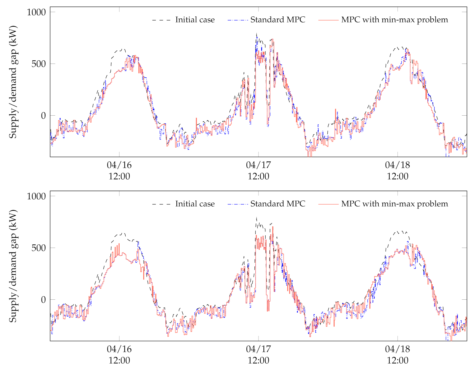
5.3. Contribution of the Worst-Case Approach

It should be noted here that the main optimisation problem responsible for balancing power supply and demand in the power distribution grid, as constructed in Section 4.2, prioritises constraints so that the volume ones are always upheld. In other words, in cases where no feasible solution is found, voltage constraints are relaxed in order to guarantee that biogas volume constraints and water volume constraints are always upheld. For this reason, hereinafter, only voltage constraint violation is examined to evaluate the efficiency of the proposed min–max problem in enhancing the control strategy’s robustness to forecasting errors.

In this section, the amended predictive control strategy as explained above is implemented, and its results are presented and discussed in comparison with three other cases:

• Case 1. The initial case where no optimisation is carried out. The biogas plant has a constant power generation output. The water tower is subject to an ON/OFF controller, which activates its pump when a low-level sensor is triggered and deactivates it when a high-level sensor is triggered;
• Case 2. The predictive control strategy described in Section 4, with GPR forecasts of the PV power generation, grid load, and water demand used;
• Case 3. The amended control strategy proposed in this paper, based on the addition of the min–max problem to anticipate the worst-case scenario within the forecasts’ confidence intervals in terms of constraint violation.

For each case, a simulation is run over a week in April. This period is selected because it presents high PV power generation and therefore demonstrates significant voltage overshooting. Two sizes of sliding windows are used for the MPC scheme in the results that are presented hereinafter: a 4 h window and a 10 h window. These two sliding window sizes are chosen to examine the difference in effects of the min–max problem on the MPC strategy’s performance for both short sliding windows and long ones. The evaluation metrics of the MPC scheme with both sliding window sizes are assembled in

Table 1. Assessment of the min–max problem’s contribution to the control strategy’s robustness to forecasting errors, for a week in April. See below (Section 5.3) for details about the three cases. For Case 2 and Case 3, 4 h and 10 h sliding windows are considered.

Evaluation Metric	Case 1	Case 2		Case 3
		4-h	10-h	4-h	10-h
$\sqrt{f_{obj,final}}$ ($\mathrm{k}\mathrm{W}$)	10,035	8984	8700	8966	8648
$\kappa$ (–)	–	40,872	385,320	39,700	358,990
${\Omega }_{P_{\mathrm{PV}}^{risk}}$ ($\mathrm{k}\mathrm{W}$)	–	–	–	16.26	19.41
${\Omega }_{P_{cons}^{risk}}$ ($\mathrm{k}\mathrm{W}$)	–	–	–	5.56	6.73
${\Omega }_{Q_{w,out}^{risk}}$ (${\mathrm{m}}^3{\mathrm{h}}^{-1}$)	–	–	–	−4.24 × 10−15	−6.41 × 10−16
$\nu$ (%)	23.71	5.36	6.85	4.96	6.35
$\Phi$ ($\mathrm{k}\mathrm{V}$)	4371.4	1632.7	1464.6	1464.5	1176.8

.

When examining the inner-workings of the min–max problem, it can be deduced that there are noteworthy deviations between forecasted values of PV power generation and grid load and the ones corresponding to worst-case scenarios. For the considered week, for the tested MPC windows of 4 h and 10 h, the deviation of worst-case scenario PV power generation values from the forecasted values (${\Omega }_{P_{\mathrm{PV}}}$) represents, on average, 7% and 9% of the data’s mean, respectively. When it comes to the grid load, the deviation of worst-case scenario values from forecasted ones ${\Omega }_{P_{cons}}$ is less notable. For the tested MPC windows of 4 h and 10 h, it represents 3% an 2% of the data’s mean, respectively.

Having said that, forecasted values of water demand and the ones corresponding to worst-case scenarios are virtually identical (${\Omega }_{Q_{w,out}}$ is virtually null). This observation reaffirms the presumption that water demand, and by extension water levels in the water tower’s storage tank, have no direct impact on voltage fluctuations in the power distribution grid. Their influence resides solely in determining the water tower’s capacity in absorbing excess power off the grid at a given time, which can be properly foreseen through proper dimensioning of the storage tank.

The instances of voltage overshooting decrease steadily from Case 1 through Case 3. In fact, the amended MPC scheme with the min–max problem (Case 3) brings down their percentage ($\nu$) to 4.96% and 6.35% for the 4 h window and the 10 h window, respectively, from an initial value of 23.71%. The total surface area of voltage overshooting $\Phi$ is also considerably reduced from the initial value. It brought down to $1464.5$ $\mathrm{k}$$\mathrm{V}$ and $1176.8$ $\mathrm{k}$$\mathrm{V}$ for the 4 h window and the 10 h window, respectively, from an initial value of $4371.4$ $\mathrm{k}$$\mathrm{V}$.

The gain procured through the addition of the min–max problem to the MPC scheme is deduced by comparing the metrics of Case 2 and Case 3. As it happens, for the 4 h sliding window, voltage overshooting is further decreased from Case 2 to Case 3 by $168.2$ $\mathrm{k}$$\mathrm{V}$, which amounts to 3.8% of the total surface area of voltage overshooting in the initial case. Percentage-wise, this decrease corresponds to 0.4% of the initial instances of overshooting.

For the 10 h sliding window, voltage overshooting is decreased from Case 2 to Case 3 by $287.8$ $\mathrm{k}$$\mathrm{V}$, which amounts to 6.6% of the total surface area of voltage overshooting in the initial case. Percentage-wise, this decrease corresponds to 0.5% of the initial instances of overshooting. The small fraction of the eliminated instances of overshooting with respect to the corresponding percentage of reduced surface area suggests that the min–max problem is particularly apt in eliminating major overshooting incidents. Table 1 reveals that the drop in the total surface area of voltage overshooting observed between the scheme using a 4 h window and the one using a 10 h window is accompanied by an increase in the percentage of instances of overvoltage. Figure 10 illustrates the extrema of voltage fluctuations within the power distribution grid for the standard MPC strategy and the one using a min-max problem, for both sliding window sizes (4 h and 10 h). Voltage overshooting is considerably reduced in both cases with respect to the initial case. Voltage values mostly remain within the acceptable voltage bounds and veer closer to the nominal value (230 $\mathrm{V}$). Unfortunately, this is achieved at the expense of the smoothness of the voltage curves. A possible solution to this issue could be the addition of a regularisation term to the objective function in order to penalise high-frequency voltage fluctuations. That being said, several voltage fluctuations are eliminated thanks to the addition of the min–max problem to the control strategy. This is especially noticeable for the MPC scheme using a 10 h window where notable overshooting incidents are removed during midday of 16 April and 18 April.

The addition of the min–max problem does not introduce additional computational burden to the control strategy. In fact, the computational complexity (measured by $\kappa$) decreases from Case 2 to Case 3 by 2.9% for the scheme using a 4 h window and by 6.8% for the scheme using a 10 h window. Figure 11 displays the evolution of the gap between power supply and demand for MPC schemes with and without the min–max problem. It is clear that neither scheme succeeds in reducing this gap significantly. However, they trim the peak occurring everyday around noon, due to the peak in PV power generation. This trimming effect is more visible for the scheme using a 10 h window than the one using a 4 h window. This is reflected in the the final values of the objective function. Though reduced from the initial case, they change very little between Case 2 (MPC using GPR forecasts) and Case 3 (MPC using GPR forecasts and the min–max problem). This suggests that the min–max problem does not provoke any degradation to the MPC strategy’s ability to reduce the gap between supply and demand in the power distribution grid.

In the case study considered here, it can be seen that the MPC strategy’s reduction of the gap between supply and demand remains humble. This may be traced back to the dimensioning of the flexible assets, especially the dimensioning of these assets’ storage units. One could argue that the power generation capacity of the chosen biogas plant and the power demand capacity of the chosen water tower are too small to have any meaningful impact on the reduction of the supply/demand gap within the power distribution grid. This observation further illustrates the importance of optimal dimensioning of flexible assets in order for the smart management scheme to yield efficient results.

5.4. Discussion

The introduction of the worst-case scenario approach, detailed in Section 4.3, is inspired by previous works on min–max optimisation for uncertain nonlinear systems under constraints, which is by definition a conservative risk aversion technique. It is chosen for its relative ease of implementation and is used in this paper to complement the previously developed predictive control strategy in order to anticipate the worst-case scenario, in terms of stochastic input values, and minimise resulting voltage overshooting. The conservativeness of the technique is lessened by its containment to the following time step instead of the entire forecast horizon. This is done primarily to reduce the computational burden added by the min–max problem, in light of the real-time aspect of the application at hand. Nevertheless, the merit of extending the min–max problem to the entire forecast horizon and a quantification of its added cost are valid questions worth investigating in a follow-up to this work. It is worth mentioning that, on top of reducing voltage overshooting, the min–max problem has virtually no effect on the reduction of the gap between power supply and demand.

It is clear that both the growing power demand and the deployment of distributed generation within power distribution grids are not slowing down in the near future. Therefore, configurations like the one studied herein will likely materialise in the upcoming years, accompanied by emerging constraints such as the ones observed in this study. This goes to show the pertinence of studies such as this one in order to prepare for this inevitability.

The damper on the control scheme’s performance in the configuration studied in this paper can be traced back, at least partially, to the flexible assets’ dimensioning and their suitability to the task. As grid load and PV power generation levels rapidly rise, the flexible assets’ room for manoeuvring diminishes. Consequently, two critical questions transpire. The first question is that of optimal dimensioning of these flexible assets. In this study, the control strategy operates at the level of the MV/LV transformer. However, in an application with finer spatial granularity, this question also encompasses optimal placement of the assets within the grid. The second question is that of the assets nature and their suitability to the application.

The combination of a biogas plant and a water tower in this case study was selected in an attempt to utilise small-scale assets compatible with the rural setting of the “Smart Occitania” project and offer the possibility of deferment of the assets’ operation. Having said that, the examination of this duo’s potential reveals several flaws. To begin, the water tower’s ON/OFF operation adds computational complexity to the optimisation problem and is therefore a handicap to the real-time aspect of the applications. Besides, it infers choppier setpoints, which not only worsen voltage fluctuations but also shorten the equipment’s life expectancy.

This is especially problematic when the installation’s latitude in terms of storage levels is limited. Furthermore, flexible assets need to be extensible in order to adapt their room for manoeuvring to the rapidly growing power demand and distributed generation levels within the grid with minimal cost. The assets considered herein are not easily extensible, particularly the biogas plant, whose energy source is based on a fairly delicate organic process.

In the case of model-based predictive control applications for power grids, choosing the time step is a pivotal task with no definitive answer. A compromise is always made between the high computational cost of this type of control scheme and the granularity of the model, which allows us to capture a maximum of phenomena occurring in the system. This type of control strategy is also dependent upon access to data, in real-time, which comes with its own set of technical issues. Solutions to these issues are starting to come together through the maturing of advanced metering infrastructures in recent years.

The 10 min time step considered in this work is very much an instance of the aforementioned compromise. It allows the necessary computations of both the forecast module and the optimisation problem to run their course. However, it limits the strategy’s visibility into the high-dynamics of power grids and thus makes it impossible to intervene between two sampling times. This type of strategy can therefore be seen as an-upper level control scheme, to be coupled with longer-term planning strategies and lower-level operation methods that have the capacity to react to rapid electrical phenomena, namely methods that fall under the umbrella of electrotechnical engineering.

6. Conclusions and Prospects

The work presented in this manuscript falls within the scope of the “Smart Occitania” project, whose goal is to demonstrate the feasibility of the smart grid concept for rural and suburban low-voltage power distribution grids. To this end, a simulated case study is constructed, based on data collected during the project’s run and made available by ENEDIS, in order to elaborate a predictive control strategy for more efficient management of power flows within a power distribution grid with prolific levels of distributed generation, namely PV power generation.

The premise of the proposed strategy is to use a model-based predictive controller to optimise setpoints of flexible assets present in the power distribution grid, in order to reduce the gap between supply and demand. This optimisation is constrained by pre-defined acceptable voltage margins, in addition to the assets’ operational restrictions.

A forecast module is constructed using Gaussian process regression and provides intraday forecasts of grid load, water demand, and GHI from which PV power generation is inferred. The quality of the forecasts decreases as the forecast horizon grows longer, but quickly stabilizes around a constant error value. The GPR models also provide confidence intervals associated with the forecasts. Herein, the computed confidence intervals correspond to a probability of 95% of containing the measurements.

An evaluation is carried out of the MPC strategy’s resilience to forecasting errors, and the induced errors are quantified. Results show that the predictive control strategy is inherently resilient to forecasting errors as the final objective function value varies little between the case where measurements are used and the one where GPR forecasts are used.

Finally, a min–max problem is added upstream of the main optimisation problem. Its purpose is to anticipate and minimise the voltage overshooting resulting from forecasting errors. In this min–max problem, the feasible space defined by the confidence intervals of the forecasts is searched, in order to determine the worst-case scenario in terms of constraint violation, over the next time step. Then, the main optimisation problem incorporates this information into its decision-making process. Results show that these incidents are indeed reduced thanks to the min–max problem, both in terms of frequency of their occurrence and the total surface area of overshooting.

There are several axes along which the present work can make headway. To begin, the optimisation problem could be modified to take into account the implementability of the flexible assets’ setpoints. For example, this could take the form of a multi-objective optimisation that balances out sometimes-conflicting goals.

In addition, the min–max problem integrated into the predictive control strategy in order to improve the scheme’s resilience to forecasting errors, can be extended from focusing on the next time step to span the entire forecast horizon. The length of the min–max problem’s forecast horizon would be another parameter to be optimised. This will inevitably increase the computational burden of the control scheme, but should also enhance its performance through a better anticipation of issues that may arise along the forecast horizon, especially in light of the degradation of the forecasts’ quality as the algorithm advances into the forecast horizon.

References

- Direction Technique ENEDIS. Principes D’étude et de Développement du Réseau Pour le Raccordement des Clients Consommateurs et Producteurs BT; Technical Report; ENEDIS: Paris La Défense, France, 2018. [Google Scholar]
- Abdi, H.; Beigvand, S.D.; La Scala, M. A review of optimal power flow studies applied to smart grids and microgrids. Renew. Sustain. Energy Rev. 2017, 71, 742–766. [Google Scholar] [CrossRef]
- Syranidis, K.; Robinius, M.; Stolten, D. Control techniques and the modeling of electrical power flow across transmission networks. Renew. Sustain. Energy Rev. 2018, 82, 3452–3467. [Google Scholar] [CrossRef]
- De Oliveira-De Jesus, P.M.; Henggeler Antunes, C. A detailed network model for distribution systems with high penetration of renewable generation sources. Electr. Power Syst. Res. 2018, 161, 152–166. [Google Scholar] [CrossRef]
- Joshi, K.; Pindoriya, N. Advances in Distribution System Analysis with Distributed Resources: Survey with a Case Study. Sustain. Energy Grids Netw. 2018, 15, 86–100. [Google Scholar] [CrossRef]
- Frank, S.; Rebennack, S. An introduction to optimal power flow: Theory, formulation, and examples. IIE Trans. 2016, 48, 1172–1197. [Google Scholar] [CrossRef]
- Riffonneau, Y.; Bacha, S.; Barruel, F.; Ploix, S. Optimal Power Flow Management for Grid Connected PV Systems With Batteries. IEEE Trans. Sustain. Energy 2011, 2, 309–320. [Google Scholar] [CrossRef]
- Strbac, G. Demand side management: Benefits and challenges. Energy Policy 2008, 36, 4419–4426. [Google Scholar] [CrossRef]
- Palensky, P.; Dietrich, D. Demand side management: Demand response, intelligent energy systems, and smart loads. IEEE Trans. Ind. Inf. 2011, 7, 381–388. [Google Scholar] [CrossRef] [Green Version]
- Meyabadi, A.F.; Deihimi, M.H. A review of demand-side management: Reconsidering theoretical framework. Renew. Sustain. Energy Rev. 2017, 80, 367–379. [Google Scholar] [CrossRef]
- Balijepalli, V.M.; Pradhan, V.; Khaparde, S.A.; Shereef, R. Review of Demand Response under Smart Grid Paradigm. In Proceedings of the ISGT2011-India, Kollam, India, 1–3 December 2011; pp. 236–243. [Google Scholar]
- Aghaei, J.; Alizadeh, M.I. Demand response in smart electricity grids equipped with renewable energy sources: A review. Renew. Sustain. Energy Rev. 2013, 18, 64–72. [Google Scholar] [CrossRef]
- Siano, P. Demand response and smart grids—A survey. Renew. Sustain. Energy Rev. 2014, 30, 461–478. [Google Scholar] [CrossRef]
- McArthur, S.D.J.; Davidson, E.M.; Catterson, V.M.; Dimeas, A.L.; Hatziargyriou, N.D.; Ponci, F.; Funabashi, T. Multi-Agent Systems for Power Engineering Applications—Part I: Concepts, Approaches, and Technical Challenges. IEEE Trans. Power Syst. 2007, 22, 1743–1752. [Google Scholar] [CrossRef] [Green Version]
- McArthur, S.D.J.; Davidson, E.M.; Catterson, V.M.; Dimeas, A.L.; Hatziargyriou, N.D.; Ponci, F.; Funabashi, T. Multi-Agent Systems for Power Engineering Applications – Part II: Technologies, Standards and Tools for Building Multi-Agent Systems. IEEE Trans. Power Syst. 2007, 22, 1753–1759. [Google Scholar] [CrossRef] [Green Version]
- Mocci, S.; Natale, N.; Pilo, F.; Ruggeri, S. Demand side integration in LV smart grids with multi-agent control system. Electr. Power Syst. Res. 2015, 125, 23–33. [Google Scholar] [CrossRef]
- You, S.; Segerberg, H. Integration of 100% micro-distributed energy resources in the low voltage distribution network: A Danish case study. Appl. Therm. Eng. 2014, 71, 797–808. [Google Scholar] [CrossRef]
- Haque, A.N.M.M.; Nguyen, P.H.; Vo, T.H.; Bliek, F.W. Agent-based unified approach for thermal and voltage constraint management in LV distribution network. Electr. Power Syst. Res. 2017, 143, 462–473. [Google Scholar] [CrossRef] [Green Version]
- Dkhili, N.; Eynard, J.; Thil, S.; Grieu, S. A survey of modelling and smart management tools for power grids with prolific distributed generation. Sustain. Energy Grids Netw. 2020, 21, 100284. [Google Scholar] [CrossRef]
- Dkhili, N.; Salas, D.; Eynard, J.; Thil, S.; Grieu, S. Innovative application of model-based predictive control for low-voltage power distribution grids with significant distributed generation. Energies 2021, 14, 1773. [Google Scholar] [CrossRef]
- Pesaran, M.H.A.; Huy, P.D.; Ramachandaramurthy, V.K. A review of the optimal allocation of distributed generation: Objectives, constraints, methods, and algorithms. Renew. Sustain. Energy Rev. 2017, 75, 293–312. [Google Scholar] [CrossRef]
- Sugihara, H.; Yokoyama, K.; Saeki, O.; Tsuji, K.; Funaki, T. Economic and efficient voltage management using customer-owned energy storage systems in a distribution network with high penetration of photovoltaic systems. IEEE Trans. Power Syst. 2013, 28, 102–111. [Google Scholar] [CrossRef]
- Karimyan, P.; Gharehpetian, G.B.; Abedi, M.R.; Gavili, A. Long term scheduling for optimal allocation and sizing of DG unit considering load variations and DG type. Int. J. Electr. Power Energy Syst. 2014, 54, 277–287. [Google Scholar] [CrossRef]
- Bruni, G.; Cordiner, S.; Mulone, V.; Rocco, V.; Spagnolo, F. A study on the energy management in domestic micro-grids based on model predictive control strategies. Energy Convers. Manag. 2015, 102, 50–58. [Google Scholar] [CrossRef]
- Prodan, I.; Zio, E. A model predictive control framework for reliable microgrid energy management. Int. J. Electr. Power Energy Syst. 2014, 61, 399–409. [Google Scholar] [CrossRef]
- Vazquez, S.; Leon, J.I.; Franquelo, L.G.; Rodriguez, J.; Young, H.A.; Marquez, A.; Zanchetta, P. Model predictive control: A review of its applications in power electronics. IEEE Ind. Electron. Mag. 2014, 8, 16–31. [Google Scholar] [CrossRef]
- Tøndel, P.; Johansen, T.A. Complexity reduction in explicit linear model predictive control. IFAC Proc. Vol. 2002, 35, 189–194. [Google Scholar] [CrossRef] [Green Version]
- Belotti, P.; Kirches, C.; Leyffer, S.; Linderoth, J.; Luedtke, J.; Mahajan, A. Mixed-integer nonlinear optimization. Acta Numer. 2013, 22, 1–131. [Google Scholar] [CrossRef] [Green Version]
- Burer, S.; Letchford, A.N. Non-convex mixed-integer nonlinear programming: A survey. Surv. Oper. Res. Manag. Sci. 2012, 17, 97–106. [Google Scholar] [CrossRef] [Green Version]
- Lee, J.; Leyffer, S. Mixed Integer Nonlinear Programming; Springer: New York, NY, USA, 2012. [Google Scholar]
- Nocedal, J.; Wright, S.J. Numerical Optimization; Springer: New York, NY, USA, 2006. [Google Scholar]
- Tawarmalani, M.; Sahinidis, N.V.; Sahinidis, N. Convexification and Global Optimization in Continuous and Mixed-Integer Nonlinear Programming: Theory, Algorithms, Software, and Applications; Springer Science & Business Media: New York, NY, USA, 2002; Volume 65. [Google Scholar]
- Sahinidis, N. Mixed-integer nonlinear programming 2018. Optim. Eng. 2019, 20, 301–306. [Google Scholar] [CrossRef] [Green Version]
- Trespalacios, F.; Grossmann, I. Review of mixed-integer nonlinear and generalized disjunctive programming methods. Chem. Ing. Tech. 2014, 86, 991–1012. [Google Scholar] [CrossRef]
- Bemporad, A.; Morari, M. Robust model predictive control: A survey. In Robustness in Identification and Control; Springer: Berlin/Heidelberg, Germany, 1999; pp. 207–226. [Google Scholar]
- Mayne, D.Q.; Seron, M.M.; Raković, S. Robust model predictive control of constrained linear systems with bounded disturbances. Automatica 2005, 41, 219–224. [Google Scholar] [CrossRef]
- Di Cairano, S.; Bernardini, D.; Bemporad, A.; Kolmanovsky, I.V. Stochastic MPC with learning for driver-predictive vehicle control and its application to HEV energy management. IEEE Trans. Control. Syst. Technol. 2013, 22, 1018–1031. [Google Scholar] [CrossRef]
- Köhler, J.; Soloperto, R.; Müller, M.A.; Allgöwer, F. A computationally efficient robust model predictive control framework for uncertain nonlinear systems. arXiv 2019, arXiv:1910.12081. [Google Scholar] [CrossRef] [Green Version]
- Fioriti, D.; Poli, D. A novel stochastic method to dispatch microgrids using Monte Carlo scenarios. Electr. Power Syst. Res. 2019, 175, 105896. [Google Scholar] [CrossRef]
- Lucia, S.; Finkler, T.; Basak, D.; Engell, S. A new robust NMPC scheme and its application to a semi-batch reactor example. IFAC Proc. Vol. 2012, 45, 69–74. [Google Scholar] [CrossRef]
- Lucia, S.; Andersson, J.A.; Brandt, H.; Diehl, M.; Engell, S. Handling uncertainty in economic nonlinear model predictive control: A comparative case study. J. Process. Control. 2014, 24, 1247–1259. [Google Scholar] [CrossRef]
- Raimondo, D.M.; Limon, D.; Lazar, M.; Magni, L.; ndez Camacho, E.F. Min-max model predictive control of nonlinear systems: A unifying overview on stability. Eur. J. Control. 2009, 15, 5–21. [Google Scholar] [CrossRef]
- Limón, D.; Alamo, T.; Salas, F.; Camacho, E.F. Input to state stability of min–max MPC controllers for nonlinear systems with bounded uncertainties. Automatica 2006, 42, 797–803. [Google Scholar] [CrossRef] [Green Version]
- Skoplaki, E.; Palyvos, J.A. On the temperature dependence of photovoltaic module electrical performance: A review of efficiency/power correlations. Sol. Energy 2009, 83, 614–624. [Google Scholar] [CrossRef]
- Jakhrani, A.Q.; Othman, A.K.; Rigit, A.R.H.; Samo, S.R. Comparison of Solar Photovoltaic Module Temperature Models. World Appl. Sci. J. (Special Issue Food Environ.) 2011, 14, 1–8. [Google Scholar]
- Tolba, H.; Dkhili, N.; Nou, J.; Eynard, J.; Thil, S.; Grieu, S. GHI forecasting using Gaussian process regression: Kernel study. IFAC-PapersOnLine 2019, 52, 455–460. [Google Scholar] [CrossRef]
- Gbémou, S.; Tolba, H.; Thil, S.; Grieu, S. Global horizontal irradiance forecasting using online sparse Gaussian process regression based on quasiperiodic kernels. In Proceedings of the 2019 IEEE International Conference on Environment and Electrical Engineering and 2019 IEEE Industrial and Commercial Power Systems Europe (EEEIC/I&CPS Europe), Genova, Italy, 4–10 June 2019. [Google Scholar]
- Tolba, H.; Dkhili, N.; Nou, J.; Eynard, J.; Thil, S.; Grieu, S. Multi-Horizon Forecasting of Global Horizontal Irradiance Using Online Gaussian Process Regression: A Kernel Study. Energies 2020, 13, 4184. [Google Scholar] [CrossRef]
- Rasmussen, C.E.; Williams, C.K.I. Gaussian Processes for Machine Learning; The MIT Press: Cambridge, MA, USA, 2006. [Google Scholar]
- Khosravi, A.; Nahavandi, S.; Creighton, D.; Atiya, A.F. Lower upper bound estimation method for construction of neural network-based prediction intervals. IEEE Trans. Neural Netw. 2010, 22, 337–346. [Google Scholar] [CrossRef] [PubMed]