
Performance of a Portable FT-NIR MEMS Spectrometer to Predict Soil Features


1
Department of Agricultural and Forestry Sciences (DAFNE), University of Tuscia, 01100 Viterbo, Italy
2
Consiglio Nazionale delle Ricerche-Institute of Methodologies for Environmental Analysis (C.N.R.-IMAA), 00133 Roma, Italy
*
Author to whom correspondence should be addressed.
Soil Syst. 2022, 6(3), 66; https://doi.org/10.3390/soilsystems6030066
Submission received: 22 July 2022
/
Revised: 4 August 2022
/
Accepted: 6 August 2022
/
Published: 8 August 2022
Abstract
:NIR spectrometers based on micro-electromechanical systems (MEMS) have become available in the market, with lower prices and smaller dimensions than traditional spectrometers. MEMS technology allows for miniaturizing and reduces the cost of the spectrometers, allowing a wider use for agricultural consultants, technicians, and scientific researchers. The aim of this work was to evaluate an innovative FT-NIR MEMS spectrometer, namely the Neospectra Scanner (NS), covering the range from 1350 to 2500 nm. The assessment was performed by comparing the accuracy of prediction of soil organic carbon, texture fractions, and total calcium carbonate, obtained with NS, with that of a standard full VIS-NIR spectrometer, namely the ASD-Fieldspec Fr Pro (AF). A dataset of 182 soil samples, dried and sieved at 2 mm, collected from 4 different agricultural areas of Italy were scanned with both devices. AF showed slightly higher R2 and lower prediction error (RMSEP) than NS for all soil features, but the accuracy of the two instruments can be considered comparable. Removing the 350–1350 nm range from VIS-NIR spectra of AF, i.e., as to have the same spectral range of NS, made the prediction accuracy of AF reduced spectra (1350–2500 nm) slightly lower than that of NS. This demonstrates that the lower accuracy of the NS in soil features prediction is not due to the lower resolution of the spectra, but probably due to the lack of visible and beginning of the NIR range (350–1300 nm).

1. Introduction
Detailed maps of soil spatial variability are fundamental to support precision agriculture practices, in particular precision seeding, fertilization, and irrigation [1]. Although several covariates, based on proximal and/or remote sensing, could be used to increase the accuracy of spatial variability, the frequency of sampling for soil laboratory analysis is often strongly affected by the available budget [2,3]. Soil laboratory analyses are expensive and time-consuming, therefore, the datapoints to analyze should be very carefully selected and they should be highly representative of the spatial variability [2]. In addition, limiting the number of sampling points can reduce the representativeness of the samples and make unsuitable the interpolation of the data by geostatistical methods [3,4]. Previous research on geostatistics and soil mapping recommended at least 100 observations to calculate a reliable semi-variogram [5]. For all these reasons, it is fundamental to find methods that increase the number of analyzed datapoints without increasing the cost.
During the last decades, visible and near infrared (VIS-NIR) spectroscopy techniques have gained popularity for soil analysis because of their rapid and low-cost acquisition methods. Today, VIS-NIR spectroscopy is considered a valuable alternative to laboratory wet chemistry analyses to predict several characteristics of soil [6], particularly organic carbon (SOC) [7,8], but also texture [9], calcium carbonate (CaCO3), cation exchange capacity (CEC), and total nitrogen (TN) [10,11,12,13]. This technique has the advantage of very limited or none sample preparation, rapid and non-destructive measurements, and the potential to analyze several soil properties simultaneously. VIS-NIR spectroscopy extracts information from the sample through vibrational excitations of some molecular bonds after the absorbance of light. The resulting diffuse reflectance spectrum produces characteristic absorptions and shapes correlated with chemical–physical properties of the soil [6]. Most of the studies on soil spectroscopy use the wavelength range 350–2500 nm, which includes the visible (350–750 nm), the near infrared in the strict sense (750–1000 nm), and the short-wave infrared (SWIR 1000–2500 nm). Although the visible range provided important information on soil color and iron oxide content, most of the characteristic soil chromophores are within the SWIR range, in particular from 1400 to 2500 nm [14]. However, the reflectance spectra of soil in the VNIR (350–1000 nm) are largely non-specific because of the overlapping absorption peaks of the soil constituents.
The most important peak for water and OH– ions in secondary clay minerals is present at 1903 nm [11,13], but secondary peaks are at 1400 (OH– in water) and 2200 nm [14,15]. Several bands are also present beyond 2000 nm, and they correspond to the vibrational stretching of clays and carbonate minerals. In particular, the peak at 2342 nm is due to C-O stretching mode in the calcium carbonate molecule [8], while absorptions near 2200 nm are due to Al–OH bends, as in clay minerals kaolinite, montmorillonite, and illite [6]. Bands around 1600, 1700 to 1800, 2000, and 2200 to 2400 nm have been identified as being particularly important for SOC and TN [6].
Recently, technological development has allowed the fabrication of small-sized NIR spectrometers at much lower costs than traditional spectrometers. Such devices are based on “micro-electromechanical systems” (or MEMS) usually based on an interferometer, usually composed of oscillating mirrors and beam splitter, as well as an InGAs photodetector. The light reflected by the samples is split by a beam splitter into two light beams: one is directed to a fixed mirror, while the other is incident to a movable mirror [16]. When the beams are reflected by mirrors, they recombine at the beam splitter, producing a positive and negative interference pattern (interferogram) due to the varying path difference traveled by the two beam components. The interferogram is a diagram in the time domain; therefore, it should be transformed in the frequency domain by the Fourier transformation [17]. The strengths of FTIR spectroscopy are the improvement in signal-to-noise ratio and a significant reduction in scan time, and it has been widely used in laboratory spectroscopy for soil science since 1990 [18]. In contrast to the mature design of FTIR laboratory spectrometers, hand-held and miniaturized FT-NIR MEMS spectrometers have been optimized and commercialized only recently [19]. Therefore, the performance and applicability of such innovative hand-held spectrometers must be evaluated in specific contexts.
The aim of this work was to test the use of an innovative hand-held FT-NIR MEMS spectrometer, namely the Neospectra Scanner (Si-Ware, Menlo Park, CA, USA), to predict several soil features, namely clay, silt, and sand content, as well as SOC and CaCO3. The results of such FT-NIR MEMS spectrometer were also compared with the prediction accuracy of one of the most widely used portable VIS-NIR spectrometers, i.e., the ASD Fieldspec Fr Pro (Malvern Panalytical Ltd., Malvern, UK). According to a recent review [20], which summarizes the results of the last 20 years of soil spectroscopy, the most popular instruments for this type of application were the ASD FieldSpec (39% of the papers) and the FOSS NIR System (21% of the papers).
The Neospectra Scanner, like other FT-NIR MEMS-based spectrometers, is about 8 to 10 times cheaper, smaller, and lighter than most of the conventional spectrometers used in soil sciences. A few very recent papers testing the accuracy of such innovative miniaturized spectrometers based on FT-NIR MEMS technology have shown promising results for the application of these sensors in soil sciences [21,22,23,24].
2. Materials and Methods
2.1. Study Areas, Soil Sampling, and Analysis
This work was based on the soil sampling of four different agricultural areas in Italy, namely Jolanda di Savoia, Castelluccio di Norcia, Maccarese, and Pignola (Figure 1). The Jolanda di Savoia site (Lat. 44.87° N, Lon. 11.97° E, alt. −2 m a.s.l.) is located in the Po valley plain in the North of Italy. The area, formerly marshland, was characterized by an important reclamation starting from the end of the 19th Century, and the soils span between Mollic Thionic Fluvisol, Sapric Histosols, Vertic Endogleyic Cambisols, and Fluvic Gleysols (https://agri.regione.emilia-romagna.it/Suoli/, accessed on 21 July 2022), according to IUSS WRB classification [25].
The Castelluccio di Norcia area (Lat. 42.82° N, Lon. 13.20° E, alt. 1452 m a.s.l.) is situated in a wide intra-mountain basin characterized in the Umbria Region in Central Italy. It is characterized by Haplic and Gleyic Umbrisols, Phaeozems, Calcaric, and Eutric Cambisols developed on fluvio-lacustrine deposits and slope deposits (https://siat.regione.umbria.it/webgisru/, accessed on 21 July 2022).
The Maccarese S.p.A. farm (Lat. 41.87° N, Lon. 12.22° E, alt. 8 m a.s.l.) is located in the coastal area near Rome in Central Italy. The site is within a completely flat agricultural area, originating from land reclamation works carried out mainly during the first decades of the 20th Century. According to the regional soil map [26], the soils of the Maccarese area varied from Dystric Arenosols developed on coastal dunes and rear dunes, as well as recent alluvial and aeolian deposits, to Eutric Endochromic Luvisols, developed on reclaimed coastal plain and fluvio-marsh sediments.
The Pignola site (Lat. 40.56° N, Long. 15.76° E, alt. 816 m a.s.l.) is located in the Basilicata Region of Southern Italy. The soils of the Pignola area correspond to Eutric Vertic Cambisols, generally characterized by decarbonization and brunification processes on fluvio-lacustrine deposits [27].
A total number of 182 samples were collected at the four sites. In particular, 80 samples were obtained from Maccarese (Rome, MAC), 65 from Jolanda di Savoia (Ferrara, JOL), 26 from Pignola (Potenza, PIG), and 11 from Castelluccio di Norcia (Perugia, CAST). More detailed information of the study sites of Maccarese (Rome) and Pignola (Potenza) was also reported in a recent publication by Mzid et al. (2022) [28].
The soil samples were air-dried, crushed, and sieved at 2 mm for traditional laboratory analysis and for spectroscopy. Traditional laboratory analysis included: (i) soil texture by pipette method, according to the USDA textural thresholds; (ii) total organic carbon content by the Walkley–Black method; (iii) calcium carbonate content by the gas-volumetric method using a Dietrich–Fruhling calcimeter. The procedures of these analyses followed the official Italian methods for soil analysis implemented by the Italian Ministry of Agriculture [29].
2.2. FT-NIR MEMS Spectrometer and Spectra Acquisitions
The FT-NIR MEMS spectrometer used for this work was the Neospectra Scanner device (NS) produced by Neospectra Si-Ware Systems (Menlo Park, CA, USA). The device is based on a single-chip Michelson interferometer, composed of a fixed mirror and an oscillating mirror that represents the movable arm of the interferometer. The light is detected by an InGaAs photodetector, from which the spectrum is calculated via the Fourier transformation (www.si-ware.com, accessed on 21 July 2022). The device also integrates a light source, two internal rechargeable batteries, Bluetooth connectivity, and a white reference for reflectance. The spectrometer covers a spectral range from 1350 to 2500 nm (7400 to 4000 cm−1), with a resolution of 16 nm, for a total of 72 measured bands. The measured bands were then interpolated by polynomial regression to obtain spectra based on 252 bands and an interpolated resolution of 4.5 nm. The diameter of the collected light beam is approximately 10 mm. The NS is rugged for external applications and can be connected by bluetooth to a tablet or smartphone to record spectral data through a specific Android app provided by Neospectra.
For spectra acquisition, the soil samples were air-dried and sieved through a 2 mm sieve, then about 5 g of sieved soil was placed in a laboratory glass dish (Figure 2). NS was supplied with a sample holder, a sort of plastic ring that connects the samples to the spectrometer window, avoiding the disturbance of the external light. The spectrometer window was put in contact with the soil sample. All the soil samples were scanned in triplicate, moving the sampling probe window to a different location for each scan; the average value of the three spectra was used for elaboration. The decision of three replicates of spectral scanning was driven by a compromise between the fair representativeness of the soil samples and the speed of the analysis.
The white standard provided by Neospectra was used as a reference for reflectance, and the white reference calibration was carried out every 10 samples (30 spectral measurements). White reference (WR) measurements are needed to convert the measured radiance to relative reflectance.
To compare the performance of NS, the same soil samples were scanned by ASD Fieldspec Fr Pro (AF) following the contact probe protocol internal soil standard (ISS) of Ben Dor et al. (2015) [30], applying the reference Wylie Bay white sand as reference. The spectral resolution of AF is 3 nm in the range 350–1050 nm and 10 nm in the range 1050–2500 nm.
The 350–2500 nm spectral range was measured and converted to reflectance using a calibrated white Spectralon (Labsphere, Inc., North Sutton, NH, USA) as a WR panel. To prepare and control the experimental conditions, the AF was turned on at least 60 min before the readings started to warm up the spectrometers and the contact probe’s lamp. The room was kept dark during the readings to avoid any interference with the instrument. To prepare the soil sample readings, the following operations were performed: (i) mixing and flattening the soil within a bowl with a glass surface, (ii) bringing the samples to the ASD contact probe (CP) using an elevator, while the CP was held firmly in place, (iii) putting the soil in contact with the CP and performing the reading, and (iv) repeating the first three steps a total of five times per soil sample. For every five samples analyzed, a check with a Spectralon panel was made to check the white reference stabilization. If not, the white reference was re-acquired to set it back again to 100% to correct the detector jump. Measures were further normalized with respect to the reference soil standard according to the ISS protocol [30].
The ISS samples of Lucky Bay (LB) and Wylie Bay (WB) were also acquired to periodically perform the alignment correction of the spectra to minimize the systematic effect (i.e., to standardize the readings). The standardization followed [28]. The five spectral replicates for each soil sample were averaged, and each spectrum was associated with the sample id and its physical and chemical properties, constituting the laboratory dataset.
Reflectance values between 350 and 2500 nm were recorded with a spectral sampling of about 1 nm. The beginning and the end of each spectrum which showed a large noise were removed, obtaining spectra with a range from 450 to 2450 nm.
Although NS spectral collection was performed using a different WR and no ISS standardization method [30], it was not relevant for the aim of this study. Indeed, this work wanted to test the efficiency of NS to predict soil features but did not aim to create a standardized spectral library, also because NS has a different spectral range and resolution of full Vis-NIR spectrometers.
2.3. Spectral Pre-Processing, Model Calibration, and Validation
The spectra collected by the two devices were processed following the same procedure as described below.
The reflectance (R) spectra were converted to absorption, A = log(1/R). Then, the standard normal variate (SNV) transformation was applied. SNV removes scatter effects from spectra by centering and scaling each individual spectrum, by the formula:
where SSNV is the corrected spectrum, Si is the i-th spectrum, μ and σ are respectively the mean and the standard deviation of the spectra dataset. The Savitzky–Golay (S-G) smoothing filter was also used as a pre-treatment of the spectra, using a polynomial regression between 11 points.
Partial least square regression (PLSR) was used to calibrate the predictive models for clay, silt, sand, SOC, and CaCO3. This multivariate method is the most widely used for the prediction of soil features from VIS-NIR spectra [31] and, in general, in infrared spectroscopy [32]. The prediction is achieved by extracting from the set of predictor variables (X, spectra) a set of orthogonal factors or principal components (PCs), which have the best predictive power for the variable of interest (Y, soil feature). Therefore, the PCs of PLSR are determined not only by the predictive variables (as in principal component regression, PCR) but also by their relationships with the response variable.
The success of this multivariate technique in spectroscopy is due to several reasons, among which: it can analyze data with numerous X variables and with strong collinearity, noise scarcely influences the results of the model, the factors are determined not only by the predictor variables (as in principal component regression) but also by the response variable [32].
The software used for pre-processing of the spectra and PLSR was The Unscrambler 9.7, CAMO software, Norway. The software also implemented Martens’ Uncertainty Test [33] as a testing method to validate the PLSR models through cross-validation based on the Jack-knife principle. For this work, 10-fold cross-validation was selected.
To determine the performance of the two spectrometers and to evaluate the accuracy of the predictive models, the following statistical indices have been used:
- -
- Coefficient of determination (R2), which explain how the regression predictions approximate the real data points;
- -
- Root mean square error of prediction (RMSEP), which indicates the average absolute deviance between the predicted and observed values, is calculated as:
- -
- Ratio of performance to interquartile (RPIQ) range Q75–Q25, which indicates the precision of the prediction, defined by RMSEP compared with the Q25-Q75 interquartile range of the observed values, calculated as:
In soil spectroscopy, RPIQ was introduced by Bellon-Maurel (2010) [34] in substitution of the ratio of performance to deviation (RPD), which was commonly used to evaluate the predictive models based on spectroscopy. The authors criticized the use of RPD, based on the standard deviation of the observed values because the standard deviation does not correctly describe the spread of the population in non-parametric and skewed populations. The higher the RPIQ, the more accurate the predictive models are in relation to the soil dataset’s variance. Several articles reported satisfactory accuracy of soil spectroscopy predictive models for RPIQ > 2 and very high accuracy for RPIQ > 3 [35,36,37,38,39].
3. Results
Soil Features Statistical Distribution
The soil samples selected for this study were collected within four important agricultural areas in Northern, Central, and Southern Italy, representing a good degree of diversity. The whole dataset consisted of 182 samples with a wide range of variation (Table 1) and satisfactory representativeness of the soils of the Italian agricultural context in terms of texture, SOC, and total carbonates (CaCO3). The coefficient of variation (CV%) spanned from a minimum of 46% for clay to a maximum of 90% and 137% for SOC and CaCO3, respectively.
The clay and silt data are very close to normal distribution, whereas the SOC showed a higher frequency of low values, as confirmed by the positive skewness of the descriptive statistics (Table 1). In addition, sand and CaCO3 showed a bimodal distribution, with high frequency in low and high values: for example, for CaCO3, several values were equal to zero. The SOC data distribution could be quasi-normalized by a natural logarithmic transformation (SOC_ln) (Figure 3). Therefore, we tested the models of SOC prediction using both the original and the ln-transformed data. Natural logarithmic transformation was also tested for sand and CaCO3, but the results in terms of normalization and improvements in PLSR prediction were not satisfactory, therefore, the non-transformed data were used in this work.
The spectra collected by AF and NS devices did not show any evident outliers (Figure 4), therefore, they were all used for PLSR predictions. The clearest peaks for both instruments were around 1450, 1900 and 2200 nm, which represent the typical and most important absorbance peaks of soil spectroscopy [6]. In particular, 1450 and 1900 nm represent the main peaks of hydroxyl (-OH) in water, organic matter, and clay minerals, as well as carbonyl (C=O) in organic matter [8,14,35,40]. The absorbance peak around 2200 nm is more influenced by OH- and Al-OH bonds of clay minerals, as well as CH- bond of aliphatic compounds of organic matter [14].
The results of PLSR predictive models for SOC, SOC_ln (normalized), clay, silt, sand, and CaCO3 are summarized in Table 2. AF showed slightly higher R2 and lower RMSE than NS for all the soil features, but the accuracy of the two instruments can be considered comparable. The difference in the value of the RPIQ between the AF and NS varied from a maximum of 0.76 for sand prediction to a minimum of 0.06 for CaCO3. Logarithmic transformation of SOC (SOC_ln) improved the accuracy of prediction for both instruments, increasing R2 from 0.76 to 0.82 and from 0.81 to 0.88 for NS and AF, respectively.
Using the reduced bandwidth 1350–2450 nm of AF, obtaining the same bandwidth of NS, the PLSR prediction accuracy decreased, although the errors can be considered quite satisfactory (Table 2). It is important to note that, although AF at the reduced spectral range of 1350–2450 nm had a higher spectral resolution (10 nm@1400/2100 nm) than NS (16 nm), the predictive models of all the soil features showed slightly lower accuracy, testified by higher RMSEP and lower R2.
4. Discussion
The results of this study demonstrate that the quality of the spectra collected by the hand-held FT-NIR MEMS spectrometer, namely the Neospectra Scanner (NS), can be compared with one of the most used full VIS-NIR spectrometers in soil science, namely the ASD-Fieldspec (AF). Using the same pre-treatment of the spectra and the PLSR models to predict soil features, the two instruments provided comparable performance, although the AF spectrometer showed slightly higher accuracy for SOC and CaCO3. This assumption is consistent with a similar previous publication conducted in Australia with a soil dataset of similar dimensions [21].
The prediction accuracy of PLSR using NS showed the highest R2 and RPIQ for SOC_ln (R2 = 0.82, RPIQ = 3.53), clay (R2 = 0.83, RPIQ = 3.84), and sand (R2 = 0.82, RPIQ = 3.17). Although silt and CaCO3 provided slightly lower RPIQ, which was 2.56 and 2.03, respectively, the prediction errors can be considered suitable for quantitative predictions, as suggested by other publications [35,36,37,38,39]. The quasi-normalization of the soil variables that showed a strong non-parametric distribution allowed to improve the PLSR prediction accuracy, as demonstrated by the results of log-normalization carried out for SOC (SOC_ln).
The accuracy of these models is consistent with the results of other publications on soil spectroscopy. Using NS in 232 samples with lower variables (SD = 0.35 g∙100 g−1), PLSR and 10-fold cross-correlation, Sharififar et al. (2019) [21] found R2 = 0.73 and RMSEP = 0.18 g∙100 g−1 for SOC prediction. A recent publication by Dhawale et al. (2022) [24] reported for prediction of clay and sand R2 = 0.82 and 0.72 and RMSEP = 7.2 and 12.7 g∙100 g−1, respectively, using a portable VIS-NIR spectrometer with 232 samples, PLSR regression, and leave-one-out cross-validation. Using AF on 148 soil samples in southern France, Adeline et al. (2017) [41] obtained using PLSR prediction of clay and CaCO3 R2 = 0.80 and 0.88, and RMSEP = 3.1 and 4.3 g 100 g−1, respectively. A recent study by Ng et al. (2020) [22] reported R2 and RMSEP of Cubist predictive models of a large (n: 1601) national spectral library of Indonesia, using the Neospectra module, later included in NS. The use of such a large spectral library with wide coefficients of variance provided R2 that varied from 0.22 (silt) to 0.57 (SOC) and RMSEP from 0.29 g·100 g−1 for SOC to 15.1 g·100 g−1 for sand.
Although the NS did not measure the visible and the beginning of the NIR range (350–1350 nm), the predictive accuracy of SOC, texture fractions, and CaCO3 appears to be satisfactory. In addition, removing the 350–1350 nm range from the VIS-NIR spectra of AF, made the prediction accuracy of this instrument slightly lower than NS, as clearly observable in Table 2. This demonstrates that the lower accuracy of the NS in soil features prediction is not due to the lower resolution of the measured spectra but probably to the lack of visible and NIR range 350–1300 nm. For SOC prediction, in particular, it is well known that the 350–1300 nm range can provide important information regarding color, often related to organic carbon, as well as the OH- bond (700 and 930 nm), the C-O-C stretching of polysaccharides, and the C=O bond of COOH [42].
Although the dataset of 182 samples is not very large, the accuracy of prediction of SOC, texture, and calcium carbonate by the NS and PLSR models seems to be very promising. It is important to highlight that such an instrument has a cost that is approximately 8–10 times lower than the most common VIS-NIR spectrometers used in soil science, such as AF. In addition, the NS weighs about 1 kg—it is compacted and without any external cables—whereas the AF weighs about 5.5 kg and is supplied by an external contact probe and cables.
Portable FT-NIR MEMS spectrometers are expected to be used more and more in the coming years, as the progress in this technology is very rapid and the quality of the spectra is increasingly comparable with the traditional full VIS-NIR spectrometers, as demonstrated by this study and other very recent papers [21,22,23]. The lowering of costs of these instruments allows for wider use in professional soil and agronomic consulting, as well as in supporting precision agriculture, making the technique exploitable also in the under-developed and developing regions of the world. Further studies should be done to test the performance of such sensors to predict other useful soil features, like total nitrogen, CEC, available potassium and phosphorous, as well as soil contaminants such as microplastic [43,44].
5. Conclusions
This study evaluated the performance of an innovative hand-held FT-NIR MEMS spectrometer with a bandwidth of 1350–2500 nm, namely the Neospectra Scanner (NS) for the prediction of soil organic carbon, texture fractions (sand, silt, and clay) and total calcium carbonate. The study compared the prediction errors with one of the most used full VIS-NIR spectrometers (350–2500 nm), namely ASD-Fieldspec Fr Pro (AF). Results demonstrated that the NS provided comparable accuracy with AF for all the soil variables studied, using PLSR as a predictive multivariate model. The slightly higher accuracy of AF seems to be due more to the longer spectral bandwidth, which includes visible and very near IR range (350–1300 nm), than to the higher spectral resolution.
The lower cost and the higher handling of NS than the other traditional field spectrometers, probably make this device more and more exploitable in soil survey and monitoring. The possibility of adding the visible range to the NS spectral bandwidth could improve the prediction of soil features. Future studies should explore the use of FT-NIR MEMS devices directly in the field, optimizing the corrective models for external disturbances, in particular, for moisture conditions.
Author Contributions
Conceptualization of the work, S.P. (Simone Priori); data curation, S.P. (Simone Priori), N.M., S.P. (Simone Pascucci) and S.P. (Stefano Pignatti); investigation: S.P. (Simone Priori); methodology, S.P. (Simone Priori), N.M., S.P. (Simone Pascucci), S.P. (Stefano Pignatti) and R.C.; project administration: R.C.; validation: S.P. (Simone Priori); visualization: S.P. (Simone Priori) and N.M.; writing—original draft preparation: S.P. (Simone Priori); writing—review and editing: S.P. (Simone Priori), N.M., S.P. (Stefano Pignatti) and R.C. All authors have read and agreed to the published version of the manuscript.
Funding
This study was co-funded by the Italian Space Agency (ASI) within the TEHRA project Contract N. 2022-6-U.0, CUP F83C22000160005.
Institutional Review Board Statement
Not applicable.
Informed Consent Statement
Not applicable.
Data Availability Statement
The data presented in this study are available on request.
Acknowledgments
The authors want to thank Giampiero Ubertini and Sara Caccia for technical assistance with the soil laboratory analysis.
Conflicts of Interest
The authors declare no conflict of interest.
References
- Gebbers, R.; Adamchuk, V.I. Precision agriculture and food security. Science 2010, 327, 828–831. [Google Scholar] [CrossRef]
- Rossel, R.V.; McBratney, A.B. Soil chemical analytical accuracy and costs: Implications from precision agriculture. Aust. J. Exp. Agric. 1998, 38, 765–775. [Google Scholar] [CrossRef]
- Wetterlind, J.; Stenberg, B.; Söderström, M. The use of near infrared (NIR) spectroscopy to improve soil mapping at the farm scale. Precis. Agric. 2008, 9, 57–69. [Google Scholar] [CrossRef] [Green Version]
- Wetterlind, J.; Stenberg, B.; Söderström, M. Increased sample point density in farm soil mapping by local calibration of visible and near infrared prediction models. Geoderma 2010, 156, 152–160. [Google Scholar] [CrossRef] [Green Version]
- Webster, R.; Oliver, M.A. Sample adequately to estimate variograms of soil properties. J. Soil Sci. 1992, 43, 177–192. [Google Scholar] [CrossRef]
- Stenberg, B.; Rossel, R.A.V.; Mouazen, A.M.; Wetterlind, J. Visible and near infrared spectroscopy in soil science. Adv. Agron. 2010, 107, 163–215. [Google Scholar]
- Li, S.; Viscarra Rossel, R.A.; Webster, R. The cost-effectiveness of reflectance spectroscopy for estimating soil organic carbon. Eur. J. Soil Sci. 2022, 73, e13202. [Google Scholar] [CrossRef]
- Gholizadeh, A.; Rossel, R.A.V.; Saberioon, M.; Borůvka, L.; Kratina, J.; Pavlů, L. National-scale spectroscopic assessment of soil organic carbon in forests of the Czech Republic. Geoderma 2021, 385, 114832. [Google Scholar] [CrossRef]
- Jaconi, A.; Vos, C.; Don, A. Near infrared spectroscopy as an easy and precise method to estimate soil texture. Geoderma 2019, 337, 906–913. [Google Scholar] [CrossRef]
- Davari, M.; Karimi, S.A.; Bahrami, H.A.; Hossaini, S.M.T.; Fahmideh, S. Simultaneous prediction of several soil properties related to engineering uses based on laboratory Vis-NIR reflectance spectroscopy. Catena 2021, 197, 104987. [Google Scholar] [CrossRef]
- Leone, A.; Viscarra-Rossel, R.; Amenta, P.; Buondonno, A. Prediction of soil properties with PLSR and vis-NIR spectroscopy: Application to mediterranean soils from Southern Italy. Curr. Anal. Chem. 2012, 8, 283–299. [Google Scholar] [CrossRef]
- Zhao, D.; Arshad, M.; Li, N.; Triantafilis, J. Predicting soil physical and chemical properties using vis-NIR in Australian cotton areas. Catena 2021, 196, 104938. [Google Scholar] [CrossRef]
- Ramirez-Lopez, L.; Wadoux, A.C.; Franceschini, M.H.; Terra, F.S.; Marques, K.P.P.; Sayão, V.M.; Demattê, J.A.M. Robust soil mapping at the farm scale with vis–NIR spectroscopy. Eur. J. Soil Sci. 2019, 70, 378–393. [Google Scholar] [CrossRef] [Green Version]
- Viscarra Rossel, R.A.; Behrens, T. Using data mining to model and interpret soil diffuse reflectance spectra. Geoderma 2010, 158, 46–54. [Google Scholar] [CrossRef]
- Ben-Dor, E.; Inbar, Y.; Chen, Y. The reflectance spectra of organic matter in the visible near-infrared and short wave infrared region (400–2500 nm) during a controlled decomposition process. Remote Sens. Environ. 1997, 61, 1–15. [Google Scholar] [CrossRef]
- Chai, J.; Zhang, K.; Xue, Y.; Liu, W.; Chen, T.; Lu, Y.; Zhao, G. Review of MEMS based Fourier transform spectrometers. Micromachines 2020, 11, 214. [Google Scholar] [CrossRef] [Green Version]
- Ismail, A.A.; van de Voort, F.R.; Sedman, J. Fourier transform infrared spectroscopy: Principles and applications. In Techniques and Instrumentation in Analytical Chemistry; Elsevier: Amsterdam, The Netherlands, 1997; Volume 18, pp. 93–139. [Google Scholar]
- Nguyen, T.T.; Janik, L.J.; Raupach, M. Diffuse reflectance infrared Fourier transform (DRIFT) spectroscopy in soil studies. Soil Res. 1991, 29, 49–67. [Google Scholar] [CrossRef]
- Beć, K.B.; Grabska, J.; Huck, C.W. Principles and applications of miniaturized near-infrared (NIR) spectrometers. Chem. A Eur. J. 2021, 27, 1514–1532. [Google Scholar] [CrossRef]
- Ahmadi, A.; Emami, M.; Daccache, A.; He, L. Soil properties prediction for precision agriculture using visible and near-infrared spectroscopy: A systematic review and meta-analysis. Agronomy 2021, 11, 433. [Google Scholar] [CrossRef]
- Sharififar, A.; Singh, K.; Jones, E.; Ginting, F.I.; Minasny, B. Evaluating a low-cost portable NIR spectrometer for the prediction of soil organic and total carbon using different calibration models. Soil Use Manag. 2019, 35, 607–616. [Google Scholar] [CrossRef]
- Ng, W.; Anggria, L.; Siregar, A.F.; Hartatik, W.; Sulaeman, Y.; Jones, E.; Minasny, B. Developing a soil spectral library using a low-cost NIR spectrometer for precision fertilization in Indonesia. Geoderma Reg. 2020, 22, e00319. [Google Scholar] [CrossRef]
- Tang, Y.; Jones, E.; Minasny, B. Evaluating low-cost portable near infrared sensors for rapid analysis of soils from South Eastern Australia. Geoderma Reg. 2020, 20, e00240. [Google Scholar] [CrossRef]
- Dhawale, N.M.; Adamchuk, V.I.; Prasher, S.O.; Rossel, R.A.V.; Ismail, A.A. Evaluation of Two Portable Hyperspectral-Sensor-Based Instruments to Predict Key Soil Properties in Canadian Soils. Sensors 2022, 22, 2556. [Google Scholar] [CrossRef]
- IUSS WRB 2015. World Reference Base for Soil Resources 2014, Update 2105. International Soil Classification System for Naming Soils and Creating Legends for Soil Maps; World Soil Resources Reports No. 106; FAO: Rome, Italy, 2015. [Google Scholar]
- Napoli, R.; Paolanti, M.; di Ferdinando, S. Atlante Dei Suoli Del Lazio; ARSIAL Regione Lazio: Rome, Italy, 2019; ISBN 978-88-904841-2-4. [Google Scholar]
- Cassi, F.; Viviano, L. I Suoli Della Basilicata—Carta Pedologica Della Regione Basilicata in Scala 1:250.000; Direzione Generale: Potenza, Italy, 2006; p. 343. [Google Scholar]
- Mzid, N.; Castaldi, F.; Tolomio, M.; Pascucci, S.; Casa, R.; Pignatti, S. Evaluation of Agricultural Bare Soil Properties Retrieval from Landsat 8, Sentinel-2 and PRISMA Satellite Data. Remote Sens. 2022, 14, 714. [Google Scholar] [CrossRef]
- Violante, P. Metodi di Analisi Chimica del Suolo; Franco Angeli editore: Milano, Italy, 2000; 496p. [Google Scholar]
- Dor, E.B.; Ong, C.; Lau, I.C. Reflectance measurements of soils in the laboratory: Standards and protocols. Geoderma 2015, 245, 112–124. [Google Scholar]
- Wold, S.; Sjöström, M.; Eriksson, L. PLS-regression: A basic tool of chemometrics. Chemom. Intell. Lab. Syst. 2001, 58, 109–130. [Google Scholar] [CrossRef]
- Abdi, H. Partial least squares regression and projection on latent structure regression (PLS Regression). Wiley Interdiscip. Rev. Comput. Stat. 2010, 2, 97–106. [Google Scholar] [CrossRef]
- Martens, H.; Martens, M. Modified Jack-knife estimation of parameter uncertainty in bilinear modelling by partial least squares regression (PLSR). Food Qual. Prefer. 2000, 11, 5–16. [Google Scholar] [CrossRef]
- Bellon-Maurel, V.; Fernandez-Ahumada, E.; Palagos, P.; Roger, J.-M.; McBratney, A.B. Critical review of chemometric indicators commonly used for assessing the quality of the prediction of soil attributes by NIR spectroscopy. TrAC Trends Anal. Chem. 2010, 29, 1073–1081. [Google Scholar] [CrossRef]
- Terra, F.S.; Demattê, J.A.; Rossel, R.A.V. Spectral libraries for quantitative analyses of tropical Brazilian soils: Comparing vis–NIR and mid-IR reflectance data. Geoderma 2015, 255, 81–93. [Google Scholar] [CrossRef]
- Clairotte, M.; Grinand, C.; Kouakoua, E.; Thébault, A.; Saby, N.P.; Bernoux, M.; Barthès, B.G. National calibration of soil organic carbon concentration using diffuse infrared reflectance spectroscopy. Geoderma 2016, 276, 41–52. [Google Scholar] [CrossRef]
- Lucà, F.; Conforti, M.; Castrignanò, A.; Matteucci, G.; Buttafuoco, G. Effect of calibration set size on prediction at local scale of soil carbon by Vis-NIR spectroscopy. Geoderma 2017, 288, 175–183. [Google Scholar] [CrossRef]
- Jiang, Q.; Li, Q.; Wang, X.; Wu, Y.; Yang, X.; Liu, F. Estimation of soil organic carbon and total nitrogen in different soil layers using VNIR spectroscopy: Effects of spiking on model applicability. Geoderma 2017, 293, 54–63. [Google Scholar] [CrossRef]
- Greenberg, I.; Seidel, M.; Vohland, M.; Koch, H.J.; Ludwig, B. Performance of in situ vs laboratory mid-infrared soil spectroscopy using local and regional calibration strategies. Geoderma 2022, 409, 115614. [Google Scholar] [CrossRef]
- Calderón, F.J.; Reeves, J.B.; Collins, H.P.; Paul, E.A. Chemical differences in soil organic matter fractions determined by diffuse-reflectance mid-infrared spectroscopy. Soil Sci. Soc. Am. J. 2011, 75, 568–579. [Google Scholar] [CrossRef] [Green Version]
- Adeline, K.R.; Gomez, C.; Gorretta, N.; Roger, J.M. Predictive ability of soil properties to spectral degradation from laboratory Vis-NIR spectroscopy data. Geoderma 2017, 288, 143–153. [Google Scholar] [CrossRef] [Green Version]
- Vohland, M.; Ludwig, M.; Thiele-Bruhn, S.; Ludwig, B. Determination of soil properties with visible to near-and mid-infrared spectroscopy: Effects of spectral variable selection. Geoderma 2014, 223, 88–96. [Google Scholar] [CrossRef]
- Crocombe, R.A. The future of portable spectroscopy. In Portable Spectroscopy and Spectrometry; Wiley: Hoboken, NJ, USA, 2021; pp. 545–571. [Google Scholar] [CrossRef]
- Wander, L.; Lommel, L.; Meyer, K.; Braun, U.; Paul, A. Development of a low-cost method for quantifying microplastics in soils and compost using near-infrared spectroscopy. Meas. Sci. Technol. 2022, 33, 075801. [Google Scholar] [CrossRef]
Figure 1.
Distribution of sampling sites. (a) Jolanda di Savoia, Ferrara (JOL); (b) Castelluccio da Norcia, Perugia (CAST); (c) Maccarese, Roma (MAC); (d) Pignola, Potenza (PIG). The white dots represent the sampling sites; in some cases, two soil samples were collected some meters apart within the sampling site to check short-range soil variability.
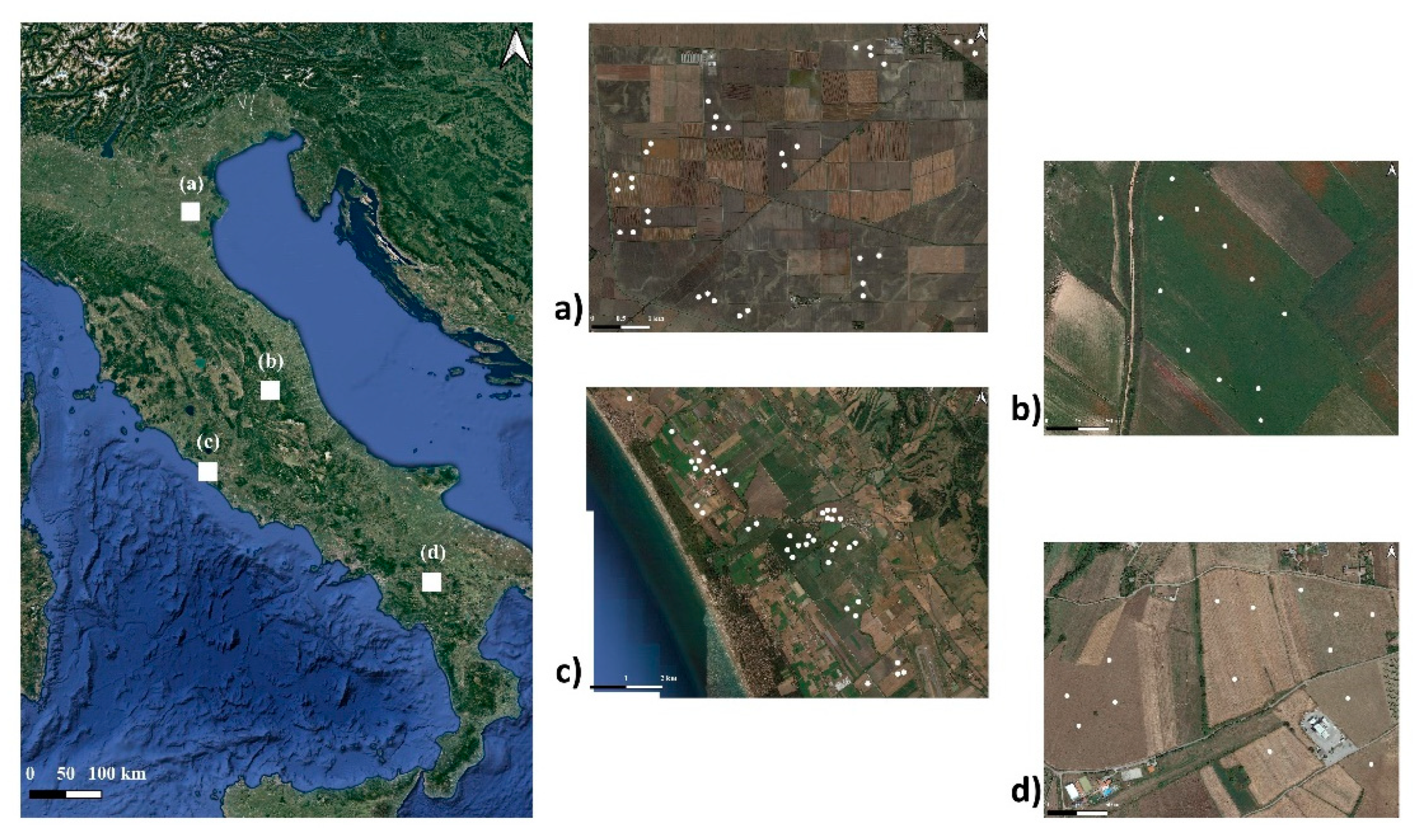
Figure 2.
The spectral measurements carried out by Neospectra Scanner. All the measurements were visualized and recorded in the dedicated Android tablet, connected by bluetooth signal.
Figure 2.
The spectral measurements carried out by Neospectra Scanner. All the measurements were visualized and recorded in the dedicated Android tablet, connected by bluetooth signal.

Figure 3.
Normal probability plot of original SOC data (a) and natural logarithmic transformed (b) data. The skewness of the data distribution moved from 1.77 (original data) to 0.27 (Ln-transformed data).
Figure 3.
Normal probability plot of original SOC data (a) and natural logarithmic transformed (b) data. The skewness of the data distribution moved from 1.77 (original data) to 0.27 (Ln-transformed data).
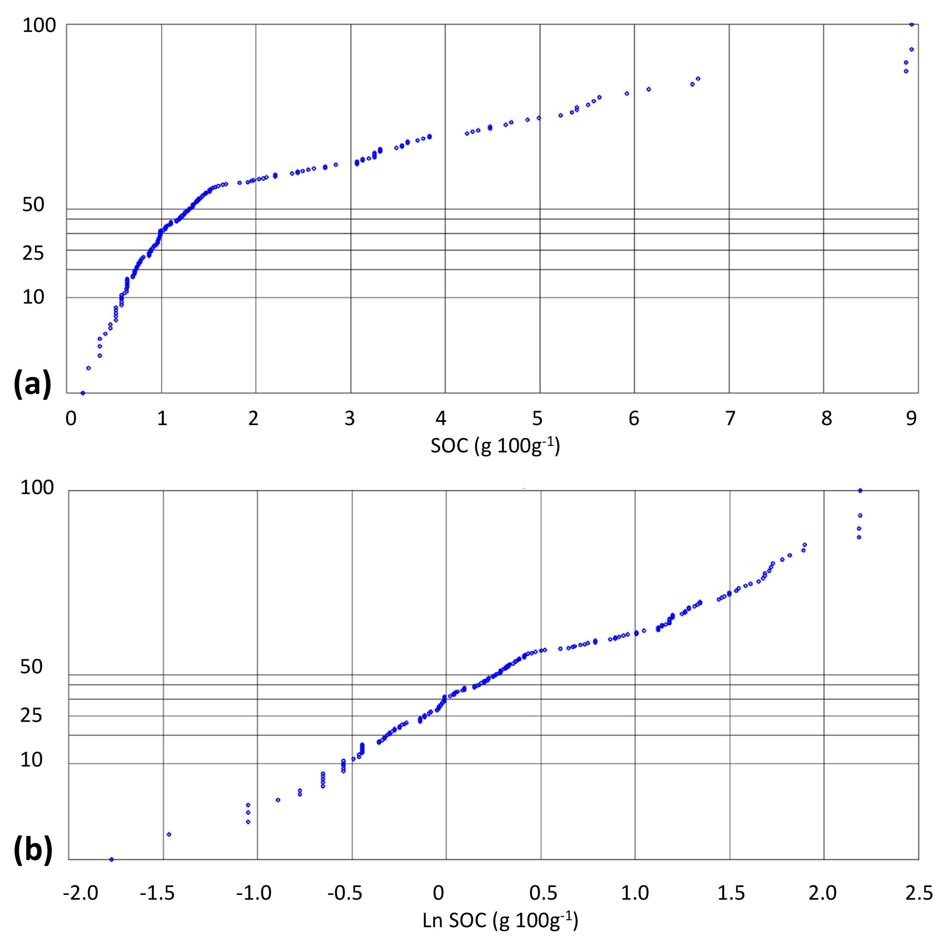
Figure 4.
Spectra graphs obtained by ASD-Fieldspec (a) and Neospectra Scanner (b). The red dashed line represents the median of the spectra.
Figure 4.
Spectra graphs obtained by ASD-Fieldspec (a) and Neospectra Scanner (b). The red dashed line represents the median of the spectra.


Table 1.
Descriptive statistics of the analyzed parameters of the soil samples used for this study. The unit measure of all the variables was g·100 g−1.
Table 1.
Descriptive statistics of the analyzed parameters of the soil samples used for this study. The unit measure of all the variables was g·100 g−1.
| n = 182 | Mean | Median | Min | Max | St.dev. | Skewness |
|---|---|---|---|---|---|---|
| Clay | 42.0 | 38.0 | 3.6 | 77.3 | 19.3 | −0.02 |
| Silt | 27.2 | 26.2 | 0.7 | 66.2 | 14.4 | 0.30 |
| Sand | 30.8 | 26.2 | 1.6 | 93.4 | 25.3 | 1.00 |
| CaCO3 | 3.5 | 1.3 | 0.0 | 22.5 | 4.8 | 1.67 |
| SOC | 2.0 | 1.3 | 0.2 | 8.9 | 1.8 | 1.80 |
Table 2.
Results of 10-fold cross-validation of the PLSR models for prediction of SOC, Clay, Silt, Sand, and CaCO3, using the spectra of the Neospectra Scanner, the whole spectrum of ASD Fieldspec, and the NIR bands 1350–2450 nm of ASD Fieldspec spectrum. PCs represent the number of principal components (or latent variables) used by the PLSR. *: the logarithmic transformation of SOC, to obtain a quasi-normal data distribution. The unit measure of all the variables was g·100 g−1.
| Neospectra Scanner (1350–2500 nm) | ASD Fieldspec (350–2500 nm) | ASD Fieldspec (1350–2500 nm) | ||
|---|---|---|---|---|
| SOC n:182 | PCs | 8 | 14 | 11 |
| R2 | 0.76 | 0.81 | 0.74 | |
| RMSEP | 0.88 | 0.78 | 0.92 | |
| RPIQ | 2.39 | 2.69 | 2.28 | |
| SOC_ln * n:182 | PCs | 7 | 15 | 10 |
| R2 | 0.82 | 0.88 | 0.78 | |
| RMSEP | 0.34 | 0.27 | 0.37 | |
| RPIQ | 3.53 | 4.44 | 3.24 | |
| Clay n:182 | PCs | 8 | 11 | 11 |
| R2 | 0.83 | 0.87 | 0.84 | |
| RMSEP | 8.08 | 7.08 | 7.67 | |
| RPIQ | 3.84 | 4.38 | 4.04 | |
| Silt n:182 | PCs | 6 | 9 | 11 |
| R2 | 0.70 | 0.79 | 0.74 | |
| RMSEP | 7.96 | 6.69 | 7.42 | |
| RPIQ | 2.56 | 3.05 | 2.75 | |
| Sand n:182 | PCs | 7 | 11 | 11 |
| R2 | 0.82 | 0.88 | 0.84 | |
| RMSEP | 10.63 | 8.57 | 10.25 | |
| RPIQ | 3.17 | 3.93 | 3.29 | |
| CaCO3 n:182 | PCs | 8 | 11 | 8 |
| R2 | 0.78 | 0.79 | 0.74 | |
| RMSEP | 2.27 | 2.20 | 2.46 | |
| RPIQ | 2.03 | 2.09 | 1.87 | |
Publisher’s Note: MDPI stays neutral with regard to jurisdictional claims in published maps and institutional affiliations. |
© 2022 by the authors. Licensee MDPI, Basel, Switzerland. This article is an open access article distributed under the terms and conditions of the Creative Commons Attribution (CC BY) license (https://creativecommons.org/licenses/by/4.0/).
Share and Cite
MDPI and ACS Style
Priori, S.; Mzid, N.; Pascucci, S.; Pignatti, S.; Casa, R. Performance of a Portable FT-NIR MEMS Spectrometer to Predict Soil Features. Soil Syst. 2022, 6, 66. https://doi.org/10.3390/soilsystems6030066
AMA Style
Priori S, Mzid N, Pascucci S, Pignatti S, Casa R. Performance of a Portable FT-NIR MEMS Spectrometer to Predict Soil Features. Soil Systems. 2022; 6(3):66. https://doi.org/10.3390/soilsystems6030066
Chicago/Turabian StylePriori, Simone, Nada Mzid, Simone Pascucci, Stefano Pignatti, and Raffaele Casa. 2022. "Performance of a Portable FT-NIR MEMS Spectrometer to Predict Soil Features" Soil Systems 6, no. 3: 66. https://doi.org/10.3390/soilsystems6030066