Article

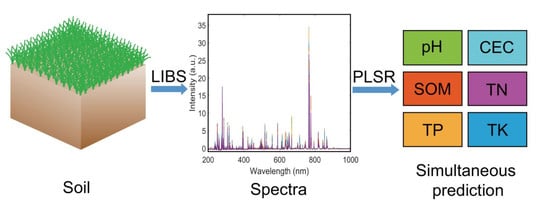
Fast and Simultaneous Determination of Soil Properties Using Laser-Induced Breakdown Spectroscopy (LIBS): A Case Study of Typical Farmland Soils in China

1
State Key Laboratory of Soil and Sustainable Agriculture, Institute of Soil Science, Chinese Academy of Sciences, Nanjing 210008, China
2
University of Chinese Academy of Sciences, Beijing 100049, China
*
Author to whom correspondence should be addressed.
Soil Syst. 2019, 3(4), 66; https://doi.org/10.3390/soilsystems3040066
Submission received: 2 July 2019 / Revised: 19 September 2019 / Accepted: 24 September 2019 / Published: 26 September 2019
(This article belongs to the Special Issue Proximal Soil Sensing Applications)

Abstract

:
Accurate management of soil nutrients and fast and simultaneous acquisition of soil properties are crucial in the development of sustainable agriculture. However, the conventional methods of soil analysis are generally labor-intensive, environmentally unfriendly, as well as time- and cost-consuming. Laser-induced breakdown spectroscopy (LIBS) is a “superstar” technique that has yielded outstanding results in the elemental analysis of a wide range of materials. However, its application for analysis of farmland soil faces the challenges of matrix effects, lack of large-scale soil samples with distinct origin and nature, and problems with simultaneous determination of multiple soil properties. Therefore, LIBS technique, in combination with partial least squares regression (PLSR), was applied to simultaneously determinate soil pH, cation exchange capacity (CEC), soil organic matter (SOM), total nitrogen (TN), total phosphorus (TP), total potassium (TK), available phosphorus (AP), and available potassium (AK) in 200 soils from different farmlands in China. The prediction performances of full spectra and characteristic lines were evaluated and compared. Based on full spectra, the estimates of pH, CEC, SOM, TN, and TK achieved excellent prediction abilities with the residual prediction deviation (RPDV) values > 2.0 and the estimate of TP featured good performance with RPDV value of 1.993. However, using characteristic lines only improved the predicted accuracy of SOM, but reduced the prediction accuracies of TN, TP, and TK. In addition, soil AP and AK were predicted poorly with RPDV values of < 1.4 based on both full spectra and characteristic lines. The weak correlations between conventionally analyzed soil AP and AK and soil LIBS spectra are responsible for the poor prediction abilities of AP and AK contents. Findings from this study demonstrated that the LIBS technique combined with multivariate methods is a promising alternative for fast and simultaneous detection of some properties (i.e., pH and CEC) and nutrient contents (i.e., SOM, TN, TP, and TK) in farmland soils because of the extraordinary prediction performances achieved for these attributes.

Graphical Abstract

1. Introduction

The traditional agricultural production system is facing a great challenge of meeting the human demand for food due to the rapid increase in world population [1,2]. It is generally accepted that developing precision agriculture, based on real-time monitoring of soil fertility, crop growth, and environmental change to increase grain production, plays a vital role in alleviating the pressure of grain demand [3,4]. As a crucial component of precision agriculture, precision management of soil nutrients requires real-time monitoring of soil nutrients by using simple, rapid, and inexpensive detection methods [5]. However, the conventional methods involving routine digestion, titration, and other preparatory procedures are generally labor-intensive, as well as time- and cost-consuming [6]. Additionally, there is the risk of environmental pollution from the emission and waste generated during these operational processes [7]. Therefore, they are unable to satisfy the needs for accurate management of soil nutrients, and more efficient methods that allow rapid, inexpensive, and environmentally friendly assessments of soil nutrients are needed for the development of precision farming and sustainable agriculture.
Laser-induced breakdown spectroscopy (LIBS), an atomic emission spectroscopy technique, has been widely used for elemental analysis of various materials since the inception of the term “LIBS” in 1981 [8]. A typical LIBS system is composed of a solid-state laser, a spectrometer, a control system, and an optical system. By focusing a high-energy laser beam on the sample surface, a plasma plume is generated on the surface, resulting in excited atomic, ionic, and molecular species [9,10]. The radiative light with various frequencies is collected by a spectrometer to form a spectrum during the cooling of the plasma. The LIBS technique has many merits for sample analysis, including the fact that it is rapid, less destructive, cost-effective, environmentally friendly, little to no sample preparation is required, and simultaneous multi-element detection can be achieved [11,12,13]. Because of these outstanding advantages, the LIBS technique has been widely applied in various fields including space exploration [14,15,16], geological surveying [11,17,18], archaeological investigation [19,20,21], environmental monitoring [22,23,24,25], materials characterization [26,27,28], food detection [29,30,31], agriculture monitoring [32,33,34], and industry monitoring [35,36].
In recent years, considerable attention has been paid to the application of the LIBS technique to the detection of soil nutrients. For example, Cremers, et al. [37] first employed LIBS to determine the total carbon in Colorado Mollisols and Los Alamos Alfisols. In their study, a strong correlation was achieved between the carbon concentrations predicted by LIBS spectra and determined by dry combustion, which indicated the feasibility of quantifying soil carbon using LIBS technique. Martin et al. successfully applied LIBS to the measurement of total carbon and nitrogen contents in 15 different soils [38]. Bricklemyer et al. also evaluated the accuracy of LIBS in measuring the soil profile of total, inorganic, and organic carbon for field-moist, intact soil cores by interrogating 78 intact soil cores from three Montana agricultural fields [39]. Many studies have applied LIBS to measure soil carbon content, and these are summarized in the review article by Senesi and Senesi [40]. For soil nitrogen, Yan et al. employed a portable LIBS to measure nitrogen in five soils collected from central Scotland, and a good correlation (R2 = 0.82) between LIBS-predicted and microanalytical content was achieved [41]. Moreover, other nutrient elements in soil, such as K, Ca, Mg, Mn, and Fe, also have been detected using the LIBS technique [42,43,44,45].
Nevertheless, the application of LIBS for the detection of soil nutrients remains an ongoing challenge. Firstly, a major limiting factor is the "matrix effects" that result from soil heterogeneity. The "matrix effects" are caused by changes in the emission line intensities of some elements in samples when the physical properties and the chemical composition of the matrix vary [46]. Previous studies have indicated that chemometrics and multivariate methods involving spectral preprocessing and calibration are efficient at reducing the “matrix effects” when applying LIBS to the determination of elements [47,48]. However, there are only a few studies combining chemometrics and LIBS for the measurements of soil properties, especially for soil nutrients. Secondly, the absence of plentiful and typical farmland soil samples in previous studies made the results nonuniversal, and the performance of LIBS should be further investigated and verified using large quantities and more types of farmland soils [49]. Thirdly, most previous studies focus on an individual soil property or element, while less study has been done on the simultaneous prediction of various properties and nutrients for farmland soils based on the LIBS technique. In this context, the simultaneous prediction of diverse properties and nutrients of large-scale farmland soils with distinct origin and nature using the LIBS technique combined with chemometrics algorithms is urgently needed.
In this study, we applied the LIBS technique to acquire soil LIBS spectra for 200 soil samples, collected from four types of typical farmland in China. Morphological weighted penalized least squares (MPLS) and wavelet transform (WT) de-noising algorithms were used for baseline correction and smoothing of acquired LIBS spectra, respectively. Principal component analysis (PCA) was carried out for exploratory data analysis and evaluation and detection of atypical values. Partial least squares regression (PLSR) was employed to build the model containing the pretreated LIBS spectra and the chemical properties analyzed in the laboratory. The built model was then used for the prediction of soil properties according to the soil LIBS spectra. The specific objectives of this study are: (1) to simultaneously predict soil properties and nutrients in various types of farmland soils using the LIBS technique and (2) to compare the prediction accuracies of full LIBS spectra and characteristic LIBS spectral lines for various soil properties and nutrients.

2. Materials and Methods

2.1. Soil Sampling and Chemical Analysis

A total of 200 topsoil samples (0–20 cm depth) were collected from four different types of farmland in China. Samples 1–50 were the Fluvo-aquic soil collected from Shandong province; samples 51–100 were paddy soil collected from Jiangsu province; samples 101–150 were red soil collected from Jiangxi province; and samples 151–200 were black soil collected from Heilongjiang province. Detailed information about these sampling sites is summarized in Table S1, Supplementary Materials. The soil samples were air-dried naturally at room temperature and then passed through a 2 mm sieve before chemical analysis. Soil pH was measured with a pH meter (PB-21, Sartorius, Goettingen, Germany) in a soil:water ratio of 1:2.5. Soil cation exchange capacity (CEC) was determined using the ammonium acetate (pH 7) method [50]. Soil organic matter (SOM) was determined using the potassium dichromatic oxidation titration method [51]. Total nitrogen (TN) was determined by the Kieldahl method with a Kjeldahl analyzer (KjeltecTM 8200, FOSS, Shanghai, China) [52]. Total phosphorus (TP) was digested using sulfuric acid and perchloric acid and was analyzed using the molybdenum antimony blue colorimetric method [53]. Total potassium (TK) was digested using hydrofluoric acid and perchloric acid and was analyzed by flame spectrometry [54]. Available phosphorus (AP) was extracted with sodium bicarbonate solution for Fluvo-aquic soil [55] and was extracted with ammonium fluoride hydrochloride solution for paddy soil, red soil, and black soil [56]. P concentration in the extracts was measured using the colorimetric method. Available potassium (AK) was extracted with 1 N ammonium acetate and was analyzed by flame spectrometry [54]. Soil tablets used for LIBS measurement were created in dimensions of 1 cm diameter and 0.25 cm thickness using a tablet machine (YP-2, Tianjin BOJUN science and technology Co., LTD, Tianjin, China) with an applied pressure of ~55 MPa for a time duration of 2 min.

2.2. LIBS System and Spectra Acquisition

The MobiLIBS system (MobiLIBS03, IVEA, Paris, France) with AnaLIBS control software was used for spectra acquisition (Figure 1). A fourth-harmonic Nd: YAG laser (Quantel, Paris, France) was operated at 580 nm with a 5 ns pulse duration to generate a laser beam with the frequency of 20 Hz, and delivery energy of 16 mJ. Soil samples were placed over an X–Y–Z manual/automatic micrometric platform, with 1.0 µm of stage travel in every coordinate axis to ensure that each laser pulse impinged on a fresh position. The laser beam was focused on the surface of the pelleted sample by a lens (focal length of 15 cm) to generate a spot with diameter of 50 µm. Plasma was produced in the ablation area and light radiated during the plasma cooling. Emitted light was collected by a collection lens and transmitted to a Mechelle 5000 Echelle spectrometer (Andor Technology, Ltd., Belfast, Northern Ireland) by a fiber optic. The resolving power of this spectrometer was λ/∆λ = 4000. An intensified charge-coupled device camera (iStar, Andor Technology, Ltd., Belfast, Northern Ireland) was used to record the diffracted light. The delay time and the gate width were controllable and were optimized to 370 μs and 7.0 ms, respectively. The wavelengths of the obtained spectrum ranged from 200 to 1000 nm, and the resolution was 0.116 nm. For each soil sample, there was a 5 × 5 matrix of shot sites on the sample surface, with three-layer shots at each site. Thus, a total of 75 LIBS spectra were obtained for each soil sample.

2.3. Spectra Preprocessing

The baseline of the LIBS spectra was corrected by an MPLS algorithm, the detailed theory of which was described by Li et al. [57]. The adjustable parameters (λ and window size) in MPLS were optimized according to the root mean square error (RMSE) and the max peak height (MPH).
R M S E = 1 n i = 1 n ( x i z i ) 2 ,
M P H = m a x ( x i z i ) ,
where x i is the ith variable of the raw spectrum, z i is the ith variable of the estimated baseline, and n is the variable number of the spectrum. The optimal baseline-corrected spectrum should have low RMSE and high MPH values. Thus, the baseline correction efficiency coefficient (BCEC) was introduced to evaluate parameter optimization efficiency. It was calculated by subtracting the scaled RMSE matrix from the scaled MPH matrix. An optimal baseline-corrected spectrum should have a high BCEC value.
B C E C = n o r m ( M P H ) n o r m ( R M S E ) .
WT is an efficient method for spectrum de-noising. The de-noising effectiveness is affected by the choice of wavelet basis function and the decomposition level. In this study, the de-noising efficiency coefficient (DEC) that related to the signal-to-noise ratio (SNR) and peak error (PE) was used to optimize the wavelet basis function and decomposition level. These parameters were calculated using the following equations:
S N R = 10   l o g ( i = 1 n x i 2 i = 1 n ( x i x i ^ ) 2 )   ,
P E = m a x i = 1 n ( | x i x ^ i | )   ,
D E C = n o r m ( S N R ) n o r m ( P E ) ,
where x i and x i ^ are the ith variable of the raw and smoothed spectra, respectively. In addition, the spectra were normalized after baseline correction and de-noising.

2.4. Calibration and Validation

The full spectral dataset was randomly divided into a calibration set (75%, 150 samples) and a validation set (25%, 50 samples). The calibration set was used for modeling, and the validation set was used for verifying the prediction performance. The predicted performances using whole LIBS spectral range (200–1000 nm) for pH, CEC, SOM, TN, TP, TK, AP, and AK were estimated. The predicted performances of the characteristic lines for soil nutrients (i.e., SOM, TN, TP, TK, AP, and AK) were also estimated and compared with those of the whole LIBS spectral range.
PLSR is a multivariate data analysis technique which generalizes and combines features from principal component analysis and multiple linear regression [58]. In this study, PLSR was used to model the calibration set, and the number of latent variables (nLVs) was determined using ten-fold cross-validation. The coefficient of determination (R2), RMSE, and residual prediction deviation (RPD) were applied to evaluate the quality and accuracy of the models. They are mathematically expressed as follow:
R 2 = 1 i = 1 N ( y i y ^ i ) 2 i = 1 N ( y i y ¯ ) 2   ,
R M S E = 1 N i = 1 N ( y i y ^ i ) 2   ,
R P D = S D R M S E ,
where y i and y i ^ are the ith measured value and the corresponding estimated value of the dependent variable (soil property), respectively, y ¯ is the average of the estimated values, N is the number of total samples, and SD is the standard deviation of the measured values. High values of R2 and RPD, along with low RMSE value indicate a robust and accurate model. In soil science, models with RPD values <1.4 are regarded as unacceptable for prediction, models with RPD values between 1.4 and 2 are supposed to have good prediction ability, and models with RPD values >2 are considered to have excellent prediction ability.
Spectral preprocessing, PLSR modeling, statistical analyses, and graph designs were completed using MATLAB R2016a software (The Math Works Inc., Natick, MA, USA).

3. Results and Discussion

3.1. Soil Properties

Table 1 contains statistics of soil properties for the calibration and validation sets. The mean, minimum, maximum, and standard deviation (SD) of all soil properties in the calibration set were similar to the corresponding values in the validation set, suggesting that it was reasonable to divide the LIBS spectra dataset into calibration and validation sets. The coefficient of variation (CV) is a normalized dispersion measure of a probability or frequency distribution and is defined as the ratio of the SD to the mean [59]. A high CV value indicates large variability in the data set. According to Wilding [60], the CV can be assigned the following classifications to rank the variability of soil properties: CV < 15%, least variable; 15% < CV < 35%, moderately variable; and CV > 35%, most variable. In this study, the variability ranking of all soil properties except pH belonged to the “most variable” classification. The large variation in soil properties was mainly due to the spatial differences between soil sampling sites.

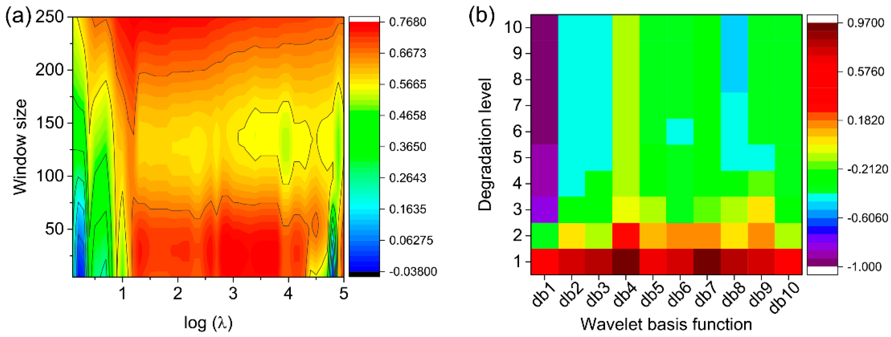
3.2. Spectra Preprocessing

Figure 2 demonstrates the comparison of original LIBS spectra and preprocessed LIBS spectra. Obviously, the baseline drift and interference line were observed in the original LIBS spectra. Baseline correction was applied first in spectral preprocessing, and the parameter optimization results are shown in Figure 3a. BCEC was highest at log(λ) value of 3 and window size of 30, indicating excellent baseline correction. Thus, λ and window size in the MPLS baseline correction algorithm were determined as 103 and 30, respectively. After that, the LIBS spectra were smoothed using the WT de-noising algorithm with a parameter optimization process. The types of wavelet basis function and degradation level were determined according to the DEC (Figure 3b). High-quality smoothing efficiency of the LIBS spectra was accomplished when the DEC value was highest. Based on this, the wavelet basis function was set as “db7” and the degradation level was set as 1.

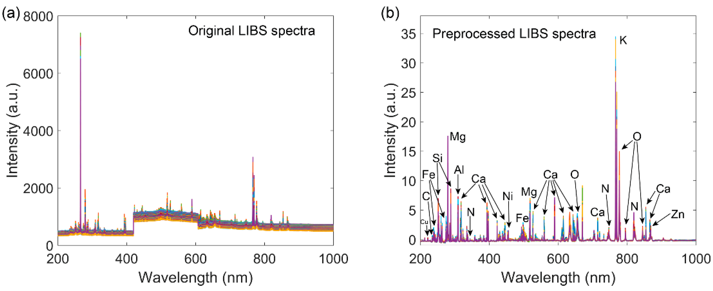
3.3. Investigation of Spectra

The preprocessed LIBS spectra of different soil samples displayed various characteristic lines at different wavelengths from 200 to 1000 nm (Figure 2b). Identifying these characteristic lines is an arduous and complicated task because of abundant characteristic emission lines as well as interference between spectral lines. In this study, the NIST Atomic Spectra Database [61] and previous studies from the literature were combined to identify the LIBS spectrum. The signal at 247.8 nm (range: 247.5–249.5 nm) was identified as the C I emission line [37,38,62]. Four emission lines were observed for O at 777.1 nm (773.4–782.9 nm), 794.6 nm (791.6–801.6 nm), 655.6 nm (649.7–664.3 nm), and 844.6 nm (840.2–848.3 nm), respectively [61,63]. Two single lines at 343.75 nm (343.2–344.6 nm) and 460.5 nm (459.8–460.9 nm) were identified as N emission lines [64]. The multilines at ranges of 739.4–755.3 nm and 815.6–828.0 nm were also confirmed as N emission lines [38,64,65,66]. Two signals at 253.7 nm (253.1–254.4 nm) and 440.2 nm (439.4–440.6 nm) were identified as the P emission lines [67,68,69,70]. Strong double peaks at 766.3 and 769.8 nm (762.6–772.8 nm) were identified as the K emission lines [68,69]. Moreover, other characteristic lines attributed to the emission lines of Na, Ca, Mg, Al, Si, and Fe were also observed, and detailed information is given in Table S1, Supplementary Materials.

3.4. PCA of LIBS Spectra

Figure 4 shows the scatter plots of the first two principal components (PCs) based on the pretreated LIBS spectra in the range of 200–1000 nm, which provided an overview map of the data structure from diverse soil spectra. The first two PCs accounted for 68.4% and 15.3% of the total variance for PC1 and PC2, respectively. From the clustering distribution, it was shown that Fluvo-aquic soil and black soil were well distinguished by PC1 from red soil and paddy soil. However, red soil and paddy soil were more difficult to be distinguished according to the first two PCs. In addition, spectral outliers can also be identified by PCA. As shown in Figure 4, the PC1–PC2 score plots of 200 samples were uniformly spread around the origin (within the circle), suggesting no spectral outlier existed in 200 LIBS spectra.

3.5. Prediction of Soil Properties

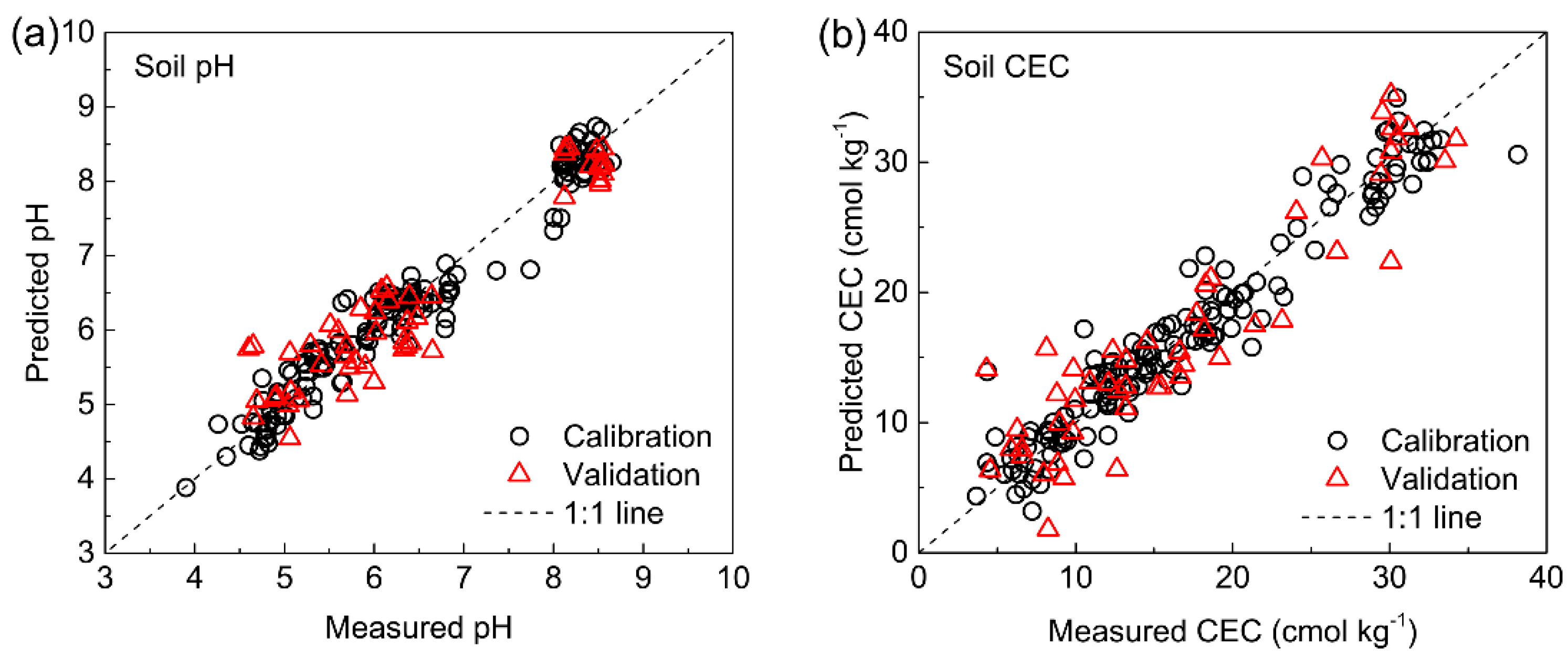
3.5.1. Soil pH and CEC
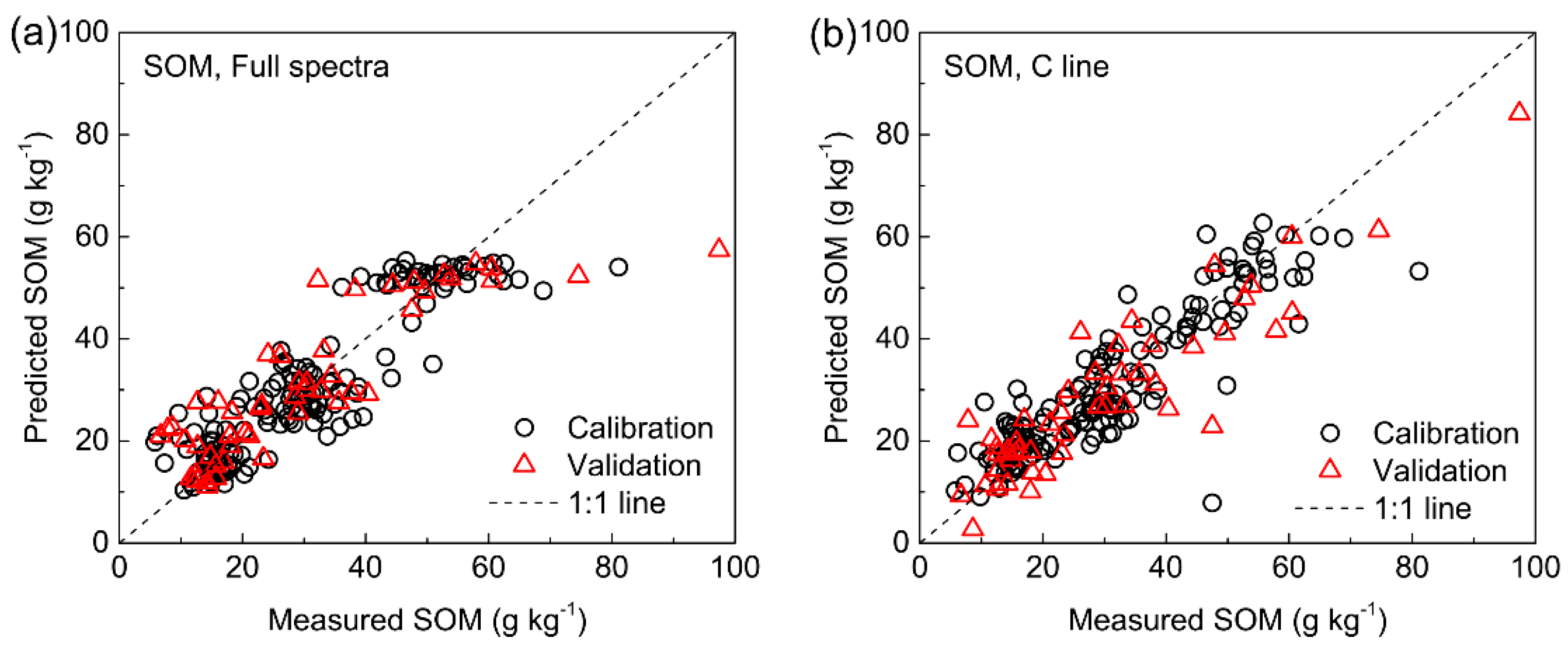
Soil pH is a crucial indicator that regulates the capacity of soils to store and supply nutrients [71] and also is the main predictor of the microbial diversity in soils [72,73]. Additionally, soil pH plays an important role in the availability and toxicity of chemical elements for plants because it affects the bioavailability of these elements in soil [74]. In the present study, we investigated the prediction performance of the full LIBS spectra for soil pH. Figure 5a shows the scatterplots of the measured versus predicted soil pH. Scatter plots in both the calibration and validation sets were located close to the 1:1 line, which indicated the robust prediction accuracy of full LIBS spectra for soil pH. The statistics for the prediction of soil pH in the calibration and validation sets as well as cross-validation are presented in Table 2. High values of RPDC (4.691) and RPDV (2.940) which were above 2.0 for prediction of soil pH were achieved, suggesting excellent prediction ability of LIBS spectra for soil pH. According to van Breemen, et al. [75], acidification or alkalization of soils occurs through H+ transfer processes involving vegetation, soil solution, and soil minerals. The acid-neutralizing capacity (ANCS) of the soil can be estimated by the component composition of the soil solid phase, as determined by total elemental analysis: ANCs = 6[Al2O3] + 2[CaO] + 2[MgO] + 2[K2O] + 2[Na2O] + 2[MnO] + 6[Fe2O3] + 2[FeO] − 2[SO3] − 2[P2O5] − [HCl]. In other words, soil pH is typically buffered by the equilibrium of the soil minerals. These minerals consume protons (H+) when they dissolve and release H+ when they precipitate, therefore buffering soil pH [76]. In this study, the importance of spectral lines according to the variable importance in the projection (VIP) scores for soil pH prediction were mainly attributed to the emission lines of mineral elements, such as K, Ca, Mg, Al, Si, and Fe, and element O (Figure S1a, Supplementary Materials), which related to the soil pH. This evidence suggested that these K, Ca, Mg, Al, Si, Fe, and O spectral lines contributed to the prediction of soil pH and gave highly interpretable variables.
Soil CEC can represent soil fertility status and influence soil structural stability, nutrient availability, soil pH, and soil chemical equilibria with fertilizers and other ameliorants [77,78]. The CEC prediction ability of the LIBS spectra using a PLSR model was studied, and the statistical results are given in Table 2. The RMSECV achieved the lowest value (3.157 cmol kg−1) when the number of latent variables (nLVs) was 10. Thus, the nLVs in the PLSR model for prediction of CEC was set to 10. The model achieved excellent prediction ability for CEC since high values of RPDV (2.507) and RV2 (0.849), as well as a low value of RMSEV (3.492 cmol kg−1), were observed. As shown in Figure 5b, the scatter plots in both the calibration and validation sets were close to the 1:1 line, which also implied the excellent performance of the model. According to VIP scores, the most important wavelengths for the prediction of CEC from the LIBS spectra mainly matched with the emission lines of soil minerals (i.e., K, Ca, Mg, Al, Si, and Fe), N, and O (Figure S1b, Supplementary Materials). This result indicated that those emission lines highly related to soil CEC. In chemical analysis, the soil CEC was measured by a total of soil exchangeable cation (i.e., K+, Na+, Ca2+, Mg2+, NH4+, H+, and Al3+), which gave an interpretation for the prediction of soil CEC based on LIBS spectra.

3.5.2. SOM

SOM is an important factor in soil quality and sustainable agriculture and it also provides feedback to environmental changes such as agricultural management change and global warming. For SOM prediction, the nLVs in the PLSR model based on full LIBS spectra and C line were set as 5 and 3, respectively, where the RMSECV (7.071 and 7.431 g kg−1) were lowest. The scatter plots of measured versus predicted SOM by PLSR models based on full LIBS spectra and the C line are shown in Figure 6, and the statistical results are presented in Table 2. Obviously, the PLSR models based on both full spectra and C line showed outstanding prediction performance for SOM because the scatter plots in the calibration and validation sets were close to the 1:1 line. However, a trend of the predicted residual with the predicted SOM content was observed in the model based on full spectra (Figure 6a). When SOM content was below 40 g kg−1, the SOM predicted values based on the full spectra had a good correlation with the chemical measured values. However, when SOM concentration was above 40 g kg−1, the predicted values of SOM based on the full spectra had a poor correlation with the chemical measured values. On the contrary, the predicted values of SOM based on C line had a good correlation with the chemical measured values within the range of SOM concentrations of 0–100 g kg−1, which indicated that the model based on C line was more robust than that based on full spectra. This is mainly because the redundant information in the full spectra will interfere with the prediction ability of the model. The introduction of irrelevant and interferential spectral lines reduced the robustness of the model, so the prediction accuracy changed with the variation of the SOM content. Compared with the model based on full spectra, the model based on C line achieved better prediction accuracy for SOM in the validation set, with RMSEV of 7.878 g kg−1, RV2 of 0.833, and RPDV of 2.373 (Table 2). However, the model based on full spectra showed poorer predicted accuracy for SOM than that based on C line. Based on full spectra, the predicted performance in the calibration set was much better than in the validation set, which indicated over-fitting of the calibration model. The larger amount of input data (5731 variables) based on the full LIBS spectra, with possibly intricate signal and noise characteristics, increased the complexity of the calibration method and gave rise to over-fitting of the calibration [79]. Generally, the risk of over-fitting can be lowered by reducing the dimensionality of the variable space [80]. Thus, the model based on the C line showed better prediction ability for SOM. This finding demonstrated that the use of the LIBS spectral C line could improve the prediction accuracy and robustness and avoid over-fitting for SOM. The prediction accuracy for SOM content in this study was comparable and often better than the accuracies obtained by other techniques for SOC and SOM with R2 values of 0.81 [81], 0.74 [82], 0.67 [83], and 0.81 [84]. There are two challenges in the application of LIBS C line to quantitative analysis of SOM content: (1) interference from Fe lines; and (2) interference from inorganic carbon in the soil. The interference by Fe lines can be easily reduced using multivariate methods. However, the interference of inorganic carbon in the soil is more difficult to eliminate. Bricklemyer et al. reported that inorganic C was best predicted by LIBS, but visible–near-infrared spectroscopy (vis–NIRS) provided better SOC predictions, which indicated that the existence of inorganic C influenced the prediction of SOM content [85]. Thus, the LIBS technique is more appropriate for SOM prediction in the soil with less inorganic carbon rather than the soil rich in inorganic carbon. However, for the soil with low SOM or high inorganic carbon, the performance of LIBS for the prediction of SOM content is subject to the interference of inorganic carbon. Therefore, combining the LIBS technique with molecular spectroscopy (such as FTIR and Raman spectra) or correcting with other elements may be alternative methods to improve the prediction ability.

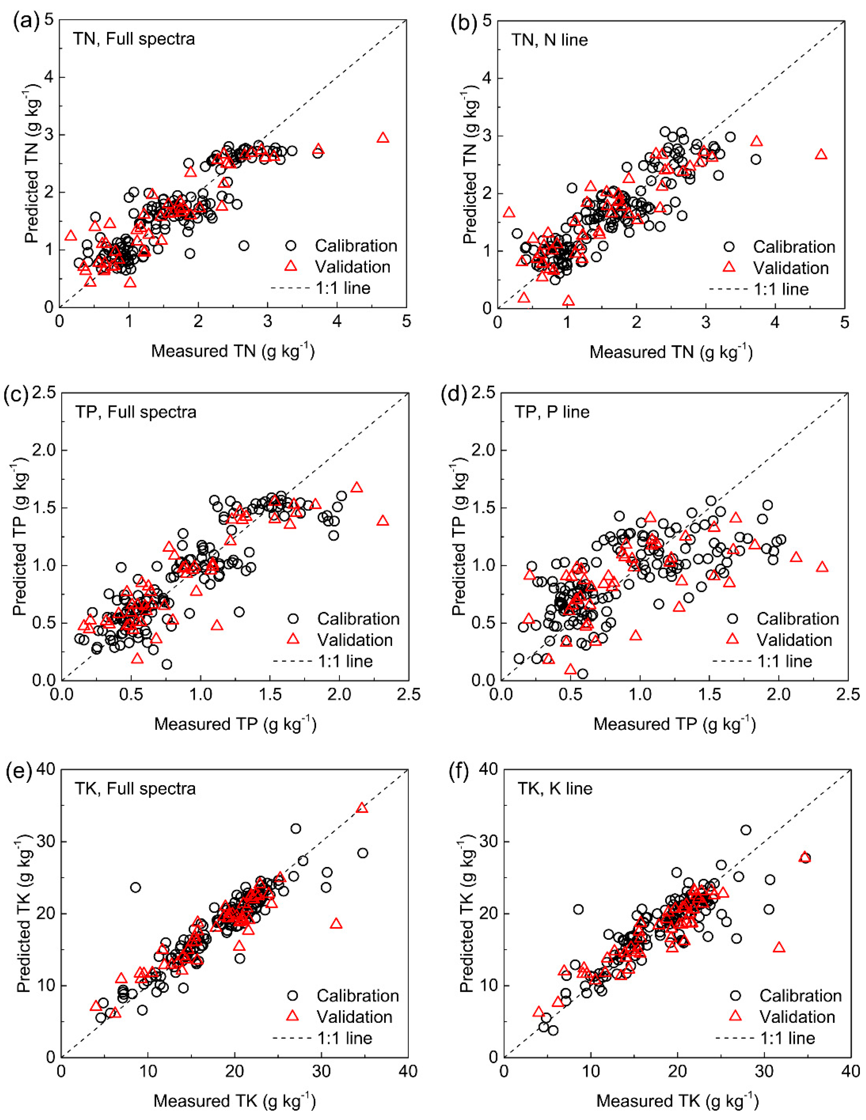
3.5.3. Soil TN, TP, and TK

In agricultural ecosystems, soil TN, TP, and TK are the major determinants and indicators of soil fertility and quality, which are closely related to soil productivity [86]. Thus, the prediction performances based on full LIBS spectra and characteristic lines for soil TN, TP, and TK were evaluated and compared (Figure 7).
For soil TN, the nLVs in PLSR models based on full spectra and N lines were optimized as 5 and 6, respectively (Table 2). The model based on full spectra achieved excellent performance since the values of RPDC (2.073) and RPDV (2.130) were both above 2.0. However, the model based on N lines only showed a good prediction ability with RPDV values of 1.849. Compared with N lines, the scatter plots based on full spectra were closer to the 1:1 line (Figure 7a,b), which also suggested better property prediction based on the full spectra for soil TN. However, trends of the predicted residual with the predicted soil TN content were also observed in the two models (Figure 7a,b), which suggested that using N lines did not improve the robustness. The relatively poor prediction accuracy based on N lines may be caused by the influence of the nitrogen (N2) in the air. Dong et al. used argon to eliminate the influence of the N2 in air and showed that the intensity of N line was strongly correlated with the N content in soil [65]. Thus, improving the measurement conditions is an effective approach for enhancing the quantitative ability of LIBS spectra with regards to soil nitrogen. As we know, soil TN is composed of N-containing compounds such as mineral and organic N, and therefore the soil TN content is also related to other mineral and organic elements. Previous studies also indicated that soil N content is strongly correlated with that of C [87]. In addition, the VIP scores of variables based on full spectra showed that the K, Ca, Mg, Al, and Si lines also dramatically contributed to the prediction of TN (Figure S1d, Supplementary Materials). This may be the main reason for the better prediction performance of TN based on full spectra.
For soil TP, the nLVs in the PLSR model were optimized as 4 and 3 for full spectra and P lines, respectively (Table 2). In comparison with full spectra, the model based on P line achieved higher values of RMSECV, RMSEC, and RMSEV (0.360, 0.338, 0.413 g kg−1, respectively) and lower values of RCV2, RC2, RV2, RPDC, and RPDV (0.395, 0.468, 0.364, 1.376, 1.201, respectively) (Table 2). The scatter plots in the calibration and validation sets based on P line were dispersedly distributed (Figure 7c,d). Trends of the predicted residual with the predicted soil TP content also were observed in these two models (Figure 7c,d), which suggested that the robustness was not enhanced using P line. These results indicated that the model based on P line was worse than that based on full spectra. In LIBS spectra, the intensity of P line at 253.1–254.5 nm was fairly low and was seriously interfered with by the Fe lines, resulting in a poor correlation between the P line and soil TP content. Soil inorganic P is mainly combined with K, Al, Ca, and Fe, and organic P is mainly combined with C, N, and O. Thus, the full spectra which contain emission lines of these elements showed better prediction performance. The high VIP scores of variables based on full spectra were observed at the wavelengths that were attributed to K, Ca, Al, Fe, C, N, and O (Figure S1e, Supplementary Materials), which also supported this explanation.
For soil TK, the optimal nLVs for modeling based on full spectra and K line were 6 and 5, respectively (Table 2). The model based on full spectra achieved excellent prediction performance with RMSEV, RV2, and RPDV values of 2.568 g kg−1, 0.821, and 2.323, respectively. However, the model based on K line showed relatively poorer results than that based on full spectra, with RMSEV, RV2, and RPDV values of 3.180 g kg−1, 0.737, and 1.876, respectively. As shown in Figure 7e,f, no trend of the predicted residual with the predicted soil TK content was observed in two models, suggesting the robustness of these two models. In addition, the scatter plots in the calibration and validation sets based on full spectra were both closer to the 1:1 line than those based on K line. This is because K line also contains some background information and matrix information, which had relevance to the substrate of soil, however, the full LIBS spectrum contains all emission lines of soil and the background information. Notwithstanding, the prediction accuracy of soil TK content in our study was still comparable and better than that reported by Viscarra Rossel et al. [88], in which the R2 of prediction was 0.29 using visible spectra (VIS), 0.47 using near-infrared spectra (NIR), and 0.38 using mid-infrared spectra (MIR), indicating that LIBS has better prediction ability of TK content than VIS, NIR, and MIR spectra.

3.5.4. Soil AP and AK

Soil AP and AK contents were also predicted by PLSR models based on full spectra and characteristic lines, and the results are presented in Figure S2, Supplementary Materials. Unfortunately, the prediction accuracies of AP and AK were both poor compared to other soil properties. Relatively low prediction abilities by spectroscopic techniques for AP and AK content also were reported in previous studies, which are summarized in Table S3, Supplementary Materials. It must be noted that the conventional soil analyses of AP and AK relate more to the element concentration in soil solution rather than to the chemistry of the soil matrix [89,90] This results in weak correlations between the values of soil properties analyzed by conventional methods with those predicted by LIBS spectra [91]. In addition, the extractable P and K make up only a small fraction of their total concentrations in the soil, thus total concentrations as indicated by total element fingerprinting in the LIBS spectra may not be good indicators of the extractable P and K [92].

3.6. Simultaneous Determination of Soil Properties

Fast, convenient, and simultaneous soil analytical techniques are needed for soil quality assessment and precision soil management. The LIBS is a fast, convenient, and simultaneously multi-element spectrum acquisition technique for soil. However, it is difficult to establish a single optimum condition for a simultaneous analysis of different elements with specific physical properties because laser pulse energy, delay time, and integration time gate are important LIBS parameters whose combination can improve the SNR of determined elemental lines and can, at the same time, damage others [93]. In fact, previous studies mostly focus on the optimization of experimental parameters for an individual property of soil (such as pH, CEC, C, N, P, K, etc.) [49,94,95,96]. Establishing optimum conditions separately for each element will make the LIBS measurement process become tedious, which is unworkable for the needs of precision agriculture. In this context, the simultaneous detection performance of multiple soil properties was evaluated using the soil LIBS spectra obtained under a single optimum condition and combined with chemometrics. The results indicated that the soil LIBS spectra obtained under a single optimum condition showed excellent prediction performance for the simultaneous detection of multiple soil properties. The LIBS technique presented the potential for fast and simultaneous determination of soil properties and nutrients, which shows great significance in the accurate management of soil nutrients and in guiding the agricultural production of precision agriculture.

4. Conclusions

Full LIBS spectra and characteristic lines and PLSR were used to predict the pH, CEC, and SOM, TN, TP, TK, AP, and AK contents of farmland soils in China. The prediction abilities of the full LIBS spectra and characteristic lines were compared. The full LIBS spectra showed excellent prediction performance for soil pH, CEC, SOM, TN, and TK and good prediction performance for soil TP. However, using characteristic LIBS spectral lines for modeling only improved the prediction accuracy of SOM, while it reduced the prediction accuracies of TN, TP, and TK. The AP and AK contents attained poor prediction abilities based on both full LIBS and characteristic lines. The inferior prediction abilities of AP and AK contents was mainly due to the weak relationships between the extractable properties and the LIBS characteristic spectra. Nevertheless, the LIBS technique still showed potential for fast and simultaneous determination of soil properties and nutrients. Future work should focus on: (1) developing and popularizing simple and convenient LIBS instruments for field use; and (2) improving the prediction performances of AP and AK contents via improving LIBS instruments and algorithms or fusing LIBS with other techniques.

Supplementary Materials

The following are available online at https://www.mdpi.com/2571-8789/3/4/66/s1, Figure S1: Variable importance in the projection (VIP) scores for the prediction of (a) pH, (b) CEC, (c) SOM, (d) TN, (e) TP, and (f) TK using PLSR model. Figure S2: Scatterplots of measured values versus predicted values of soil available P (a, b) and available K contents (c, d) using the PLSR model based on the full and characteristic LIBS spectra. Table S1: The detailed information of the sampling sites. Table S2: Identification of the LIBS emission lines based on the NIST Atomic Spectra Database and previous literature. Table S3: Summarized prediction ability of soil available P and available K by the various spectroscopic technique in previous studies.

Author Contributions

Conceptualization, C.D. and X.X.; Funding acquisition, C.D.; Investigation, X.X.; Methodology, C.D., F.M., and Y.S.; Project administration, J.Z.; Supervision, C.D. and J.Z.; Writing—original draft preparation, X.X.; Writing—review and editing, C.D.

Funding

The work was supported by the National Natural Science Foundation of China (41671238, 41977026), the National Key Basic Research Program of China (No. 2015CB150403), the “STS” Project from Chinese Academy of Sciences (KFJ-PTXM-003, KFJ-STS-QYZX-047), and the Jiangsu Demonstration Project in Modern Agriculture (BE2017388).

Conflicts of Interest

The authors declare no conflict of interest.

References

  1. Demattê, J.A.M.; Ramirez-Lopez, L.; Marques, K.P.P.; Rodella, A.A. Chemometric soil analysis on the determination of specific bands for the detection of magnesium and potassium by spectroscopy. Geoderma 2017, 288, 8–22. [Google Scholar] [CrossRef]
  2. Capmourteres, V.; Adams, J.; Berg, A.; Fraser, E.; Swanton, C.; Anand, M. Precision conservation meets precision agriculture: A case study from southern Ontario. Agric. Syst. 2018, 167, 176–185. [Google Scholar] [CrossRef]
  3. Gebbers, R.; Adamchuk, V.I. Precision agriculture and food security. Science 2010, 327, 828–831. [Google Scholar] [CrossRef] [PubMed]
  4. Huang, J.; Pray, C.; Rozelle, S. Enhancing the crops to feed the poor. Nature 2002, 418, 678–684. [Google Scholar] [CrossRef] [PubMed]
  5. Shaw, R.; Lark, R.M.; Williams, A.P.; Chadwick, D.R.; Jones, D.L. Characterising the within-field scale spatial variation of nitrogen in a grassland soil to inform the efficient design of in-situ nitrogen sensor networks for precision agriculture. Agric. Ecosyst. Environ. 2016, 230, 294–306. [Google Scholar] [CrossRef] [Green Version]
  6. Xing, Z.; Du, C.; Zeng, Y.; Ma, F.; Zhou, J. Characterizing typical farmland soils in China using Raman spectroscopy. Geoderma 2016, 268, 147–155. [Google Scholar] [CrossRef]
  7. Kaniu, M.I.; Angeyo, K.H. Challenges in rapid soil quality assessment and opportunities presented by multivariate chemometric energy dispersive X-ray fluorescence and scattering spectroscopy. Geoderma 2015, 241–242, 32–40. [Google Scholar] [CrossRef]
  8. De Lucia, F.C., Jr.; Gottfried, J.L. Rapid analysis of energetic and geo-materials using LIBS. Mater. Today 2011, 14, 274–281. [Google Scholar] [CrossRef]
  9. Miziolek, A.W.; Palleschi, V.; Schechter, I. Laser Induced Breakdown Spectroscopy (LIBS): Fundamentals and Applications; Cambridge University Press: Cambridge, UK, 2006. [Google Scholar]
  10. Radziemski, L.J.; Cremers, D.A. Handbook of Laser Induced Breakdown Spectroscopy; Wiley: New York, NY, USA, 2006. [Google Scholar]
  11. Han, D.; Joe, Y.J.; Ryu, J.-S.; Unno, T.; Kim, G.; Yamamoto, M.; Park, K.; Hur, H.-G.; Lee, J.-H.; Nam, S.-I. Application of laser-induced breakdown spectroscopy to Arctic sediments in the Chukchi Sea. Spectrochim. Acta Part B 2018, 146, 84–92. [Google Scholar] [CrossRef]
  12. Wang, T.; He, M.; Shen, T.; Liu, F.; He, Y.; Liu, X.; Qiu, Z. Multi-element analysis of heavy metal content in soils using laser-induced breakdown spectroscopy: A case study in eastern China. Spectrochim. Acta Part B 2018, 149, 300–312. [Google Scholar] [CrossRef]
  13. Juvé, V.; Portelli, R.; Boueri, M.; Baudelet, M.; Yu, J. Space-resolved analysis of trace elements in fresh vegetables using ultraviolet nanosecond laser-induced breakdown spectroscopy. Spectrochim. Acta Part B 2008, 63, 1047–1053. [Google Scholar] [CrossRef]
  14. Dell’Aglio, M.; López-Claros, M.; Laserna, J.J.; Longo, S.; De Giacomo, A. Stand-off laser induced breakdown spectroscopy on meteorites: Calibration-free approach. Spectrochim. Acta Part B 2018, 147, 87–92. [Google Scholar] [CrossRef]
  15. Moros, J.; ElFaham, M.M.; Laserna, J.J. Dual-spectroscopy platform for the surveillance of Mars mineralogy using a decisions fusion architecture on simultaneous LIBS-Raman data. Anal. Chem. 2018, 90, 2079–2087. [Google Scholar] [CrossRef]
  16. Mezzacappa, A.; Melikechi, N.; Cousin, A.; Wiens, R.C.; Lasue, J.; Clegg, S.M.; Tokar, R.; Bender, S.; Lanza, N.L.; Maurice, S.; et al. Application of distance correction to ChemCam laser-induced breakdown spectroscopy measurements. Spectrochim. Acta Part B 2016, 120, 19–29. [Google Scholar] [CrossRef]
  17. Hu, Y.; Li, Z.; Lü, T. Determination of elemental concentration in geological samples using nanosecond laser-induced breakdown spectroscopy. J. Anal. At. Spectrom. 2017, 32, 2263–2270. [Google Scholar] [CrossRef]
  18. Lü, T.; Hu, Y.; Li, Z.; Meng, J.; Zhang, C.; Hu, Z.; Liu, Y. Elemental fractionation and quantification of geological standard samples by nanosecond-laser ablation. Spectrochim. Acta Part B 2018, 143, 55–62. [Google Scholar] [CrossRef]
  19. García-Escárzaga, A.; Clarke, L.J.; Gutiérrez-Zugasti, I.; González-Morales, M.R.; Martinez, M.; López-Higuera, J.-M.; Cobo, A. Mg/Ca profiles within archaeological mollusc (Patella vulgata) shells: Laser-induced breakdown spectroscopy compared to inductively coupled plasma-optical emission spectrometry. Spectrochim. Acta Part B 2018, 148, 8–15. [Google Scholar] [CrossRef]
  20. Gaudiuso, R.; Dell’Aglio, M.; De Pascale, O.; Loperfido, S.; Mangone, A.; De Giacomo, A. Laser-induced breakdown spectroscopy of archaeological findings with calibration-free inverse method: Comparison with classical laser-induced breakdown spectroscopy and conventional techniques. Anal. Chim. Acta 2014, 813, 15–24. [Google Scholar] [CrossRef]
  21. Qi, J.; Zhang, T.; Tang, H.; Li, H. Rapid classification of archaeological ceramics via laser-induced breakdown spectroscopy coupled with random forest. Spectrochim. Acta Part B 2018, 149, 288–293. [Google Scholar] [CrossRef]
  22. Yu, X.; Li, Y.; Gu, X.; Bao, J.; Yang, H.; Sun, L. Laser-induced breakdown spectroscopy application in environmental monitoring of water quality: A review. Environ. Monit. Assess. 2014, 186, 8969–8980. [Google Scholar] [CrossRef]
  23. Ramli, M.; Khumaeni, A.; Kurniawan, K.H.; Tjia, M.O.; Kagawa, K. Spectrochemical analysis of Cs in water and soil using low pressure laser induced breakdown spectroscopy. Spectrochim. Acta Part B 2017, 132, 8–12. [Google Scholar] [CrossRef]
  24. Meng, D.; Zhao, N.; Wang, Y.; Ma, M.; Fang, L.; Gu, Y.; Jia, Y.; Liu, J. On-line/on-site analysis of heavy metals in water and soils by laser induced breakdown spectroscopy. Spectrochim. Acta Part B 2017, 137, 39–45. [Google Scholar] [CrossRef]
  25. Yi, R.; Yang, X.; Zhou, R.; Li, J.; Yu, H.; Hao, Z.; Guo, L.; Li, X.; Lu, Y.; Zeng, X. Determination of trace available heavy metals in soil using laser-induced breakdown spectroscopy assisted with phase transformation method. Anal. Chem. 2018, 90, 7080–7085. [Google Scholar] [CrossRef]
  26. Zou, L.; Kassim, B.; Smith, J.P.; Ormes, J.D.; Liu, Y.; Tu, Q.; Bu, X. In situ analytical characterization and chemical imaging of tablet coatings using laser induced breakdown spectroscopy (LIBS). Analyst 2018, 143, 5000–5007. [Google Scholar] [CrossRef]
  27. Serrano, J.; Cabalín, L.M.; Moros, J.; Laserna, J.J. Potential of laser-induced breakdown spectroscopy for discrimination of nano-sized carbon materials. Insights on the optical characterization of graphene. Spectrochim. Acta Part B 2014, 97, 105–112. [Google Scholar] [CrossRef]
  28. Liang, D.; Du, C.; Ma, F.; Shen, Y.; Wu, K.; Zhou, J. Characterization of nano FeIII-tannic acid modified polyacrylate in controlled-release coated urea by Fourier transform infrared photoacoustic spectroscopy and laser-induced breakdown spectroscopy. Polym. Test. 2017, 64, 101–108. [Google Scholar] [CrossRef]
  29. Markiewicz-Keszycka, M.; Cama-Moncunill, X.; Casado-Gavalda, M.P.; Dixit, Y.; Cama-Moncunill, R.; Cullen, P.J.; Sullivan, C. Laser-induced breakdown spectroscopy (LIBS) for food analysis: A review. Trends Food Sci. Technol. 2017, 65, 80–93. [Google Scholar] [CrossRef]
  30. Bilge, G.; Sezer, B.; Eseller, K.E.; Berberoglu, H.; Topcu, A.; Boyaci, I.H. Determination of whey adulteration in milk powder by using laser induced breakdown spectroscopy. Food Chem. 2016, 212, 183–188. [Google Scholar] [CrossRef]
  31. Casado-Gavalda, M.P.; Dixit, Y.; Geulen, D.; Cama-Moncunill, R.; Cama-Moncunill, X.; Markiewicz-Keszycka, M.; Cullen, P.J.; Sullivan, C. Quantification of copper content with laser induced breakdown spectroscopy as a potential indicator of offal adulteration in beef. Talanta 2017, 169, 123–129. [Google Scholar] [CrossRef]
  32. Peng, J.; Liu, F.; Zhou, F.; Song, K.; Zhang, C.; Ye, L.; He, Y. Challenging applications for multi-element analysis by laser-induced breakdown spectroscopy in agriculture: A review. TrAC Trends Anal. Chem. 2016, 85, 260–272. [Google Scholar] [CrossRef]
  33. Nicolodelli, G.; Senesi, G.S.; Ranulfi, A.C.; Marangoni, B.S.; Watanabe, A.; de Melo Benites, V.; de Oliveira, P.P.A.; Villas-Boas, P.; Milori, D.M.B.P. Double-pulse laser induced breakdown spectroscopy in orthogonal beam geometry to enhance line emission intensity from agricultural samples. Microchem. J. 2017, 133, 272–278. [Google Scholar] [CrossRef] [Green Version]
  34. Jull, H.; Künnemeyer, R.; Schaare, P. Nutrient quantification in fresh and dried mixtures of ryegrass and clover leaves using laser-induced breakdown spectroscopy. Precis. Agric. 2018, 19, 823–839. [Google Scholar] [CrossRef]
  35. Noll, R.; Fricke-Begemann, C.; Brunk, M.; Connemann, S.; Meinhardt, C.; Scharun, M.; Sturm, V.; Makowe, J.; Gehlen, C. Laser-induced breakdown spectroscopy expands into industrial applications. Spectrochim. Acta Part B 2014, 93, 41–51. [Google Scholar] [CrossRef]
  36. Sarkar, A.; Karki, V.; Aggarwal, S.K.; Maurya, G.S.; Kumar, R.; Rai, A.K.; Mao, X.; Russo, R.E. Evaluation of the prediction precision capability of partial least squares regression approach for analysis of high alloy steel by laser induced breakdown spectroscopy. Spectrochim. Acta Part B 2015, 108, 8–14. [Google Scholar] [CrossRef]
  37. Cremers, D.A.; Ebinger, M.H.; Breshears, D.D.; Unkefer, P.J.; Kammerdiener, S.A.; Ferris, M.J.; Catlett, K.M.; Brown, J.R. Measuring total soil carbon with laser-induced breakdown spectroscopy (LIBS). J. Environ. Qual. 2001, 30, 2202–2206. [Google Scholar] [CrossRef]
  38. Martin, M.Z.; Wullschleger, S.D.; Garten, C.T.; Palumbo, A.V. Laser-induced breakdown spectroscopy for the environmental determination of total carbon and nitrogen in soils. Appl. Opt. 2003, 42, 2072–2077. [Google Scholar] [CrossRef]
  39. Bricklemyer, R.S.; Brown, D.J.; Barefield, J.E.; Clegg, S.M. Intact soil core total, inorganic, and organic carbon measurement using laser-induced breakdown spectroscopy. Soil Sci. Soc. Am. J. 2011, 75, 1006–1018. [Google Scholar] [CrossRef]
  40. Senesi, G.S.; Senesi, N. Laser-induced breakdown spectroscopy (LIBS) to measure quantitatively soil carbon with emphasis on soil organic carbon. A review. Anal. Chim. Acta 2016, 938, 7–17. [Google Scholar] [CrossRef]
  41. Yan, X.T.; Donaldson, K.M.; Davidson, C.M.; Gao, Y.; Wu, H.; Houston, A.M.; Kisdi, A. Effects of sample pretreatment and particle size on the determination of nitrogen in soil by portable LIBS and potential use on robotic-borne remote Martian and agricultural soil analysis systems. RSC Adv. 2018, 8, 36886–36894. [Google Scholar] [CrossRef] [Green Version]
  42. He, Y.; Liu, X.; Lv, Y.; Liu, F.; Peng, J.; Shen, T.; Zhao, Y.; Tang, Y.; Luo, S. Quantitative analysis of nutrient elements in soil using single and double-pulse laser-induced breakdown spectroscopy. Sensors 2018, 18, 1526. [Google Scholar] [CrossRef]
  43. Yongcheng, J.; Wen, S.; Baohua, Z.; Dong, L. Quantitative analysis of magnesium in soil by laser-induced breakdown spectroscopy coupled with nonlinear multivariate calibration. J. Appl. Spectrosc. 2017, 84, 731–737. [Google Scholar] [CrossRef]
  44. Zhang, G.; Song, H.; Liu, Y.; Zhao, Z.; Li, S.; Ren, Z. Optimization of experimental parameters about laser induced breakdown and measurement of soil elements. Optik 2018, 165, 87–93. [Google Scholar] [CrossRef]
  45. Kim, E.-A.; Choi, J.H. Changes in the mineral element compositions of soil colloidal matter caused by a controlled freeze-thaw event. Geoderma 2018, 318, 160–166. [Google Scholar] [CrossRef]
  46. Senesi, G.S. Laser-Induced Breakdown Spectroscopy (LIBS) applied to terrestrial and extraterrestrial analogue geomaterials with emphasis to minerals and rocks. Earth-Sci. Rev. 2014, 139, 231–267. [Google Scholar] [CrossRef]
  47. Takahashi, T.; Thornton, B. Quantitative methods for compensation of matrix effects and self-absorption in laser induced breakdown spectroscopy signals of solids. Spectrochim. Acta Part B 2017, 138, 31–42. [Google Scholar] [CrossRef]
  48. Zaytsev, S.M.; Krylov, I.N.; Popov, A.M.; Zorov, N.B.; Labutin, T.A. Accuracy enhancement of a multivariate calibration for lead determination in soils by laser induced breakdown spectroscopy. Spectrochim. Acta Part B 2018, 140, 65–72. [Google Scholar] [CrossRef]
  49. Senesi, G.S.; Cabral, J.; Menegatti, C.R.; Marangoni, B.; Nicolodelli, G. Recent advances and future trends in LIBS applications to agricultural materials and their food derivatives: An overview of developments in the last decade (2010–2019). Part II. Crop plants and their food derivatives. TrAC Trends Anal. Chem. 2019, 118, 453–469. [Google Scholar] [CrossRef]
  50. Sumner, M.E.; Miller, W.P. Cation exchange capacity and exchange coefficients. In Methods of Soil Analysis Part 3—Chemical Methods; Bartels, J.M., Bigham, J.M., Eds.; Soil Science Society of America, Inc.: Madison, WI, USA, 1996; pp. 1201–1229. [Google Scholar]
  51. Walkley, A.; Black, I.A. An examination of Degtjareff method for determining soil organic matter, and a proposed modification of the chromic acid titration method. Soil Sci. 1934, 37, 29–38. [Google Scholar] [CrossRef]
  52. Pansu, M.; Gautheyrou, J. Handbook of Soil Analysis; Springer-Verlag: Heidelberg/Germany, Germany, 2007. [Google Scholar]
  53. Murphy, J.; Riley, J.P. A modified single solution method for the determination of phosphate in natural waters. Anal. Chim. Acta 1962, 27, 31–36. [Google Scholar] [CrossRef]
  54. Hanway, J.J.; Heidel, H. Soil analysis methods as used in Iowa State College Soil Testing Laboratory. Iowa Agric. 1952, 57, 1–31. [Google Scholar]
  55. Olsen, S.R.; Cole, C.V.; Watanabe, F.S.; Dean, L.A. Estimation of Available Phosphorus in Soils by Extraction with Sodium Bicarbonate; USDA Circular: Washington, DC, USA, 1954; Volume 939.
  56. Bray, R.H.; Kurtz, L.T. Determination of total, organic, and available forms of phosphorus in soils. Soil Sci. 1945, 59, 39–46. [Google Scholar] [CrossRef]
  57. Li, Z.; Zhan, D.J.; Wang, J.J.; Huang, J.; Xu, Q.S.; Zhang, Z.M.; Zheng, Y.B.; Liang, Y.Z.; Wang, H. Morphological weighted penalized least squares for background correction. Analyst 2013, 138, 4483–4492. [Google Scholar] [CrossRef]
  58. Shetty, N.; Gislum, R. Quantification of fructan concentration in grasses using NIR spectroscopy and PLSR. Field Crops Res. 2011, 120, 31–37. [Google Scholar] [CrossRef]
  59. Guo, L.; Zhao, C.; Zhang, H.; Chen, Y.; Linderman, M.; Zhang, Q.; Liu, Y. Comparisons of spatial and non-spatial models for predicting soil carbon content based on visible and near-infrared spectral technology. Geoderma 2017, 285, 280–292. [Google Scholar] [CrossRef]
  60. Wilding, L.P. Spatial Variability: Its Documentation, Accommodation and Implication to Soil Surveys; Pudoc: Wageningen, The Netherlands, 1985; pp. 166–194. [Google Scholar]
  61. Kramida, A.; Ralchenko, Y.; Reader, J.; NIST ASD Team. NIST Atomic Spectra Database (Ver. 5.6); National Institute of Standards and Technology: Gaithersburg, MD, USA, 2012. [Google Scholar]
  62. Ebinger, M.H.; Norfleet, M.L.; Breshears, D.D.; Cremers, D.A.; Ferris, M.J.; Unkefer, P.J.; Lamb, M.S.; Goddard, K.L.; Meyer, C.W. Extending the applicability of laser-induced breakdown spectroscopy for total soil carbon measurement. Soil Sci. Soc. Am. J. 2003, 67, 1616–1619. [Google Scholar] [CrossRef]
  63. Ji, Z.G.; Xi, J.H.; Mao, Q.N. Determination of oxygen concentration in heavily doped silicon wafer by laser induced breakdown spectroscopy. J. Inorg. Mater. 2010, 25, 893–895. [Google Scholar] [CrossRef]
  64. Harris, R.D.; Cremers, D.A.; Ebinger, M.H.; Bluhm, B.K. Determination of nitrogen in sand using laser-induced breakdown spectroscopy. Appl. Spectrosc. 2004, 58, 770–775. [Google Scholar] [CrossRef]
  65. Dong, D.M.; Zhao, C.J.; Zheng, W.G.; Zhao, X.D.; Jiao, L.Z. Spectral characterization of nitrogen in farmland soil by laser-induced breakdown spectroscopy. Spectrosc. Lett. 2013, 46, 421–426. [Google Scholar] [CrossRef]
  66. De Lucia, F.C., Jr.; Gottfried, J.L. Characterization of a series of nitrogen-rich molecules using laser induced breakdown spectroscopy. Propellants. Explos. Pyrotech. 2010, 35, 268–277. [Google Scholar] [CrossRef]
  67. Aras, N.; Yalçın, Ş. Rapid identification of phosphorus containing proteins in electrophoresis gel spots by laser-induced breakdown spectroscopy, LIBS. J. Anal. At. Spectrom. 2014, 29, 545–552. [Google Scholar] [CrossRef]
  68. Mansoori, A.; Roshanzadeh, B.; Khalaji, M.; Tavassoli, S.H. Quantitative analysis of cement powder by laser induced breakdown spectroscopy. Opt. Lasers Eng. 2011, 49, 318–323. [Google Scholar] [CrossRef]
  69. Sallé, B.; Cremers, D.A.; Maurice, S.; Wiens, R.C.; Fichet, P. Evaluation of a compact spectrograph for in-situ and stand-off laser-induced breakdown spectroscopy analyses of geological samples on Mars missions. Spectrochim. Acta Part B 2005, 60, 805–815. [Google Scholar] [CrossRef]
  70. Lu, C.; Wang, L.; Hu, H.; Zhuang, Z.; Wang, Y.; Wang, R.; Song, L. Analysis of total nitrogen and total phosphorus in soil using laser-induced breakdownspectroscopy. Chin. Opt. Lett. 2013, 11, 053004. [Google Scholar]
  71. Slessarev, E.W.; Lin, Y.; Bingham, N.L.; Johnson, J.E.; Dai, Y.; Schimel, J.P.; Chadwick, O.A. Water balance creates a threshold in soil pH at the global scale. Nature 2016, 540, 567. [Google Scholar] [CrossRef]
  72. Fierer, N.; Jackson, R.B. The diversity and biogeography of soil bacterial communities. Proc. Natl. Acad. Sci. USA 2006, 103, 626–631. [Google Scholar] [CrossRef] [Green Version]
  73. Lauber, C.L.; Strickland, M.S.; Bradford, M.A.; Fierer, N. The influence of soil properties on the structure of bacterial and fungal communities across land-use types. Soil Biol. Biochem. 2008, 40, 2407–2415. [Google Scholar] [CrossRef]
  74. Likar, M.; Vogel-Mikuš, K.; Potisek, M.; Hančević, K.; Radić, T.; Nečemer, M.; Regvar, M. Importance of soil and vineyard management in the determination of grapevine mineral composition. Sci. Total Environ. 2015, 505, 724–731. [Google Scholar] [CrossRef]
  75. Van Breemen, N.; Mulder, J.; Driscoll, C.T. Acidification and alkalinization of soils. Plant Soil 1983, 75, 283–308. [Google Scholar] [CrossRef]
  76. Sposito, G. The Chemistry of Soils; Oxford University Press: New York, NY, USA, 1989. [Google Scholar]
  77. Sharma, A.; Weindorf, D.C.; Wang, D.; Chakraborty, S. Characterizing soils via portable X-ray fluorescence spectrometer: 4. Cation exchange capacity (CEC). Geoderma 2015, 239–240, 130–134. [Google Scholar] [CrossRef]
  78. Shekofteh, H.; Ramazani, F.; Shirani, H. Optimal feature selection for predicting soil CEC: Comparing the hybrid of ant colony organization algorithm and adaptive network-based fuzzy system with multiple linear regression. Geoderma 2017, 298, 27–34. [Google Scholar] [CrossRef]
  79. Faber, N.M.; Rajkó, R. How to avoid over-fitting in multivariate calibration—The conventional validation approach and an alternative. Anal. Chim. Acta 2007, 595, 98–106. [Google Scholar] [CrossRef]
  80. Deng, B.-C.; Yun, Y.-H.; Liang, Y.-Z.; Cao, D.-S.; Xu, Q.-S.; Yi, L.-Z.; Huang, X. A new strategy to prevent over-fitting in partial least squares models based on model population analysis. Anal. Chim. Acta 2015, 880, 32–41. [Google Scholar] [CrossRef]
  81. Xing, Z.; Du, C.; Tian, K.; Ma, F.; Shen, Y.; Zhou, J. Application of FTIR-PAS and Raman spectroscopies for the determination of organic matter in farmland soils. Talanta 2016, 158, 262–269. [Google Scholar] [CrossRef]
  82. Shi, Z.; Ji, W.; Viscarra Rossel, R.A.; Chen, S.; Zhou, Y. Prediction of soil organic matter using a spatially constrained local partial least squares regression and the Chinese vis–NIR spectral library. Eur. J. Soil Sci. 2015, 66, 679–687. [Google Scholar] [CrossRef]
  83. Christy, C.D. Real-time measurement of soil attributes using on-the-go near infrared reflectance spectroscopy. Comput. Electron. Agric. 2008, 61, 10–19. [Google Scholar] [CrossRef]
  84. Li, S.; Shi, Z.; Chen, S.; Ji, W.; Zhou, L.; Yu, W.; Webster, R. In situ measurements of organic carbon in soil profiles using vis-NIR spectroscopy on the Qinghai–Tibet plateau. Environ. Sci. Technol. 2015, 49, 4980–4987. [Google Scholar] [CrossRef]
  85. Bricklemyer, R.S.; Brown, D.J.; Turk, P.J.; Clegg, S. Comparing vis–NIRS, LIBS, and combined vis–NIRS-LIBS for intact soil core soil carbon measurement. Soil Sci. Soc. Am. J. 2018, 82, 1482–1496. [Google Scholar] [CrossRef]
  86. Wang, Y.; Zhang, X.; Huang, C. Spatial variability of soil total nitrogen and soil total phosphorus under different land uses in a small watershed on the Loess Plateau, China. Geoderma 2009, 150, 141–149. [Google Scholar] [CrossRef]
  87. Yang, H.; Kuang, B.; Mouazen, A.M. Quantitative analysis of soil nitrogen and carbon at a farm scale using visible and near infrared spectroscopy coupled with wavelength reduction. Eur. J. Soil Sci. 2012, 63, 410–420. [Google Scholar] [CrossRef]
  88. Viscarra Rossel, R.A.; Walvoort, D.J.J.; McBratney, A.B.; Janik, L.J.; Skjemstad, J.O. Visible, near infrared, mid infrared or combined diffuse reflectance spectroscopy for simultaneous assessment of various soil properties. Geoderma 2006, 131, 59–75. [Google Scholar] [CrossRef]
  89. Janik, L.J.; Merry, R.H.; Skjemstad, J.O. Can mid infrared diffuse reflectance analysis replace soil extractions? Aust. J. Exp. Agric. 1998, 38, 681–696. [Google Scholar] [CrossRef]
  90. Soriano-Disla, J.M.; Janik, L.J.; Viscarra Rossel, R.A.; Macdonald, L.M.; McLaughlin, M.J. The performance of visible, near-, and mid-infrared reflectance spectroscopy for prediction of soil physical, chemical, and biological properties. Appl. Spectrosc. Rev. 2014, 49, 139–186. [Google Scholar] [CrossRef]
  91. Chang, C.-W.; Laird, D.A.; Mausbach, M.J.; Hurburgh, C.R. Near-infrared reflectance spectroscopy–principal components regression analyses of soil properties. Soil Sci. Soc. Am. J. 2001, 65, 480–490. [Google Scholar] [CrossRef]
  92. Towett, E.K.; Shepherd, K.D.; Sila, A.; Aynekulu, E.; Cadisch, G. Mid-infrared and total X-ray fluorescence spectroscopy complementarity for assessment of soil properties. Soil Sci. Soc. Am. J. 2015, 79, 1375–1385. [Google Scholar] [CrossRef]
  93. Ferreira, E.C.; Anzano, J.M.; Milori, D.M.B.P.; Ferreira, E.J.; Lasheras, R.J.; Bonilla, B.; Montull-Ibor, B.; Casas, J.; Neto, L.M. Multiple response optimization of laser-induced breakdown spectroscopy parameters for multi-element analysis of soil samples. Appl. Spectrosc. 2009, 63, 1081–1088. [Google Scholar] [CrossRef]
  94. Ferreira, E.C.; Ferreira, E.J.; Villas-Boas, P.R.; Senesi, G.S.; Carvalho, C.M.; Romano, R.A.; Martin-Neto, L.; Milori, D.M.B.P. Novel estimation of the humification degree of soil organic matter by laser-induced breakdown spectroscopy. Spectrochim. Acta Part B 2014, 99, 76–81. [Google Scholar] [CrossRef]
  95. Ferreira, E.C.; Neto, J.A.G.; Milori, D.M.B.P.; Ferreira, E.J.; Anzano, J.M. Laser-induced breakdown spectroscopy: Extending its application to soil pH measurements. Spectrochim. Acta Part B 2015, 110, 96–99. [Google Scholar] [CrossRef] [Green Version]
  96. Lin, Z.-X.; Liu, L.-M.; Liu, L.-W. Validation of the solidifying soil process using laser-induced breakdown spectroscopy. Opt. Laser Technol. 2016, 83, 13–15. [Google Scholar] [CrossRef]
Figure 1. Schematic diagram of the laser-induced breakdown spectroscopy (LIBS) system.
Soilsystems 03 00066 g001
Figure 2. Original LIBS spectra (a) and preprocessed LIBS spectra (b) of different farmland soils.
Soilsystems 03 00066 g002
Figure 3. Parameter optimization for baseline correction and de-noising of LIBS spectra: (a) Baseline correction efficiency coefficient (BCEC) as a function of log(λ) and window size. (b) De-noising efficiency coefficient (DEC) as a function of the types of wavelet basis function and degradation level.
Soilsystems 03 00066 g003
Figure 4. PC (principal component) score plots of LIBS spectra of various soil types.
Soilsystems 03 00066 g004
Figure 5. Scatterplots of measured versus predicted pH (a) and CEC (b) by the PLSR model based on the full LIBS spectra.
Soilsystems 03 00066 g005
Figure 6. Scatterplots of measured versus predicted SOM by the PLSR model based on the full LIBS spectra (a) and C line at the range of 247.2–248.0 nm (b).
Soilsystems 03 00066 g006
Figure 7. Scatterplots of measured versus predicted soil properties by the PLSR models: (a) TN based on the full LIBS spectra, (b) TN based on N lines at 459.8–460.9 nm and 737.9–757.2 nm, (c) TP based on full LIBS spectra, (d) TP based on P line at 253.1–254.4 nm, (e) TK based on full LIBS spectra, (f) TK based on K line at 762.6–772.8 nm.
Soilsystems 03 00066 g007
Table 1. Statistics of various soil properties in the calibration and validation sets.
IndexDatasetNSMinMaxMeanSDCV (%)
pHCalibration1503.90 8.65 6.40 1.31 20.44
Validation504.60 8.56 6.39 1.30 20.42
CEC (cmol kg1)Calibration1503.68 38.15 16.90 8.33 49.29
Validation504.31 34.24 16.82 8.75 52.02
SOM (g kg1)Calibration1505.74 81.06 30.72 15.39 50.11
Validation506.72 97.41 29.97 18.69 62.38
TN (g kg1)Calibration1500.28 3.72 1.65 0.76 45.85
Validation500.16 4.66 1.56 0.94 60.46
TP (g kg1)Calibration1500.13 2.02 0.89 0.46 51.91
Validation500.16 2.31 0.90 0.50 55.21
TK (g kg1)Calibration1504.58 34.75 18.15 5.34 29.43
Validation504.01 34.65 17.88 5.97 33.37
AP (mg kg1)Calibration1500.20 123.63 13.36 14.85 111.16
Validation500.00 126.25 16.04 20.81 129.73
AK (mg kg1)Calibration15033.10 424.05 118.38 60.42 51.04
Validation5018.34 307.88 118.24 70.90 59.96
NS, number of samples; SD, standard deviation; CV, coefficient of variation. CEC, cation exchange capacity; SOM, soil organic matter; TN, total nitrogen; TP, total phosphorus; TK, total potassium; AP, available phosphorus; AK, available potassium.
Table 2. The performance statistics for soil pH, CEC, and nutrient predictions in the calibration and validation sets using PLSR models based on the full and characteristic LIBS spectra.
PropertiesVariables RangenLVsCalibration SetValidation Set
RMSECVRCV2RMSECRC2RPDCRMSEVRV2RPDV
pH200–1000 nm100.4440.8850.2800.9544.6910.4440.8862.940
CEC(cmol kg1)200–1000 nm103.1570.8572.1850.9313.8263.4920.8492.507
SOM (g kg−1)200–1000 nm 57.0710.7896.0460.8462.5548.2970.8122.253
247.2–248.0 nm 37.4310.7677.0810.7882.1817.8780.8332.373
TN (g kg−1)200–1000 nm 50.4370.7090.3660.7662.0730.4420.7972.130
459.8–460.9, 739.4–755.3 nm 60.4510.6450.3690.7632.0590.5100.7101.849
TP (g kg−1)200–1000 nm 40.2230.7690.2220.7712.0970.2490.7561.993
253.1–254.5 nm30.3600.3950.3380.4681.3760.4130.3641.201
TK (g kg−1)200–1000 nm 62.5630.7702.1520.8382.4902.5680.8212.323
765.4–770.8 nm 52.8630.7132.6670.7512.0103.1800.7371.876
nLVs, number of latent variables; RMSECV, root mean square error of cross-validation; RMSEC, root mean square error in the calibration set; RMSEV, root mean square error in the validation set; RPDC, residual prediction deviation in the calibration set; RPDV, residual prediction deviation in the validation set.

