Realistic Compactification Models in Einstein–Gauss–Bonnet Gravity


Programa de Pós-Graduação em Física, Universidade Federal do Maranhão (UFMA), 65085-580 São Luís, Maranhão, Brazil
Particles 2018, 1(1), 36-55; https://doi.org/10.3390/particles1010004
Submission received: 30 January 2018
/
Revised: 15 February 2018
/
Accepted: 28 February 2018
/
Published: 4 March 2018
(This article belongs to the Special Issue Selected Papers from “The Modern Physics of Compact Stars and Relativistic Gravity 2017”)
Abstract
:We report the results of a study on the dynamical compactification of spatially flat cosmological models in Einstein–Gauss–Bonnet gravity. The analysis was performed in the arbitrary dimension in order to be more general. We consider both vacuum and -term cases. Our results suggest that for vacuum case, realistic compactification into the Kasner (power law) regime occurs with any number of dimensions (D), while the compactification into the exponential solution occurs only for . For the -term case only compactification into the exponential solution exists, and it only occurs for as well. Our results, combined with the bounds on Gauss–Bonnet coupling and the -term (, respectively) from other considerations, allow for the tightening of the existing constraints and forbid .
Keywords:
modified gravity; extra-dimensional models; cosmology; lovelock gravity; Gauss–Bonnet gravityPACS:
04.50.-h; 11.25.Mj; 98.80.Cq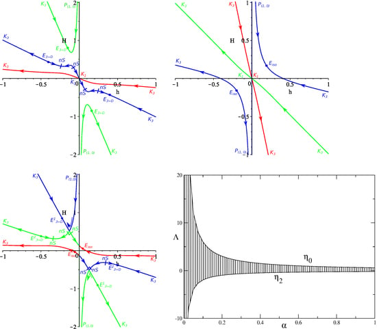
1. Introduction
It is not widely known, but the idea of extra dimensions preceded the concept of general relativity. Indeed, the first extra-dimensional model was proposed by Nordström in 1914 [1], unifying Nordström’s second gravity theory [2] with Maxwell’s electromagnetism. With time it became apparent that the true gravity theory was Einstein’s, and Kaluza [3] proposed a similar model based on General Relativity (GR): in his model five-dimensional Einstein equations could be decomposed into four-dimensional Einstein equations, in addition to Maxwell’s electromagnetism. After that, Klein [4,5] proposed a quantum mechanical interpretation of this extra dimension, and hence the Kaluza–Klein was formally formulated. Remarkably, their theory unified all known interactions at that time. With time, more interactions were known and it became clear that to unify them all, more extra dimensions are needed. Nowadays, one of the promising theories for unifying all interactions is M/string theory.
The gravitational counterpart of M/string theories often has the curvature-squared corrections in the Lagrangian to counter specific ghosts and “badly-behaving” kinetic terms. It was demonstrated [6] that the only combination of quadratic terms that leads to a ghost-free nontrivial gravitation interaction is the Gauss–Bonnet (GB) term:
Zumino [7] extended Zwiebach’s result on higher-than-squared curvature terms, supporting the idea that the low-energy limit of the unified theory might have a Lagrangian density as a sum of contributions of different powers of curvature. In this regard, Einstein–Gauss–Bonnet (EGB) gravity could be seen as a subcase of the more general Lovelock gravity [8].
All extra-dimensional theories have one thing in common—the need to explain where additional dimensions are “hiding”, as we do not sense them, at least with the current level of experiments. The generally accepted answer is that the additional dimensions are “compactified”, meaning that they are very small in size. Off course, one would want to make them small naturally, in the course of evolution and with unsuppressed initial conditions and parameters.
The cosmology with Einstein–Gauss–Bonnet gravity in extra dimensions has been actively studied for some time [9,10,11]; more recent research focuses on the power law [12,13,14,15,16,17] and exponential [17,18,19,20,21,22,23,24] solutions.
In order to find all possible regimes in the Einstein–Gauss–Bonnet cosmology, it is necessary to go beyond an exponential or power law ansatz and keep the scale factor generic. As we are particularly interested in models that allow dynamical compactification, we consider the metric as being a product of spatially three-dimensional and extra-dimensional parts. In that case, the three-dimensional part could be seen as “our Universe” and we expect this part to expand while the extra-dimensional part should be suppressed in size with respect to the three-dimensional one. In [25] we demonstrated the existence of a phenomenologically sensible regime when the curvature of the extra dimensions is negative and the Einstein–Gauss–Bonnet theory does not admit a maximally symmetric solution. In this case, both the three-dimensional Hubble parameter and the extra-dimensional scale factor asymptotically tend to the constant values. In [26] we performed a detailed analysis of the cosmological dynamics in this model with generic couplings. We recently studied this model in [27] and demonstrated that, with an additional constraint on couplings, Friedmann-type late-time behavior could be restored. Overall, the consideration of nonzero spatial curvature proved to be worthwhile. For example, for the inflaton field the spatial curvature changes the possibilities for reaching the inflation asymptotes [28,29]; in EGB gravity the spatial curvature changes the cosmological regimes [30]
The current paper is a semi-review: we review the results of [31,32,33], but also fix several inaccuracies while providing a new presentation of the results and a discussion of newly found regimes. Indeed, the original papers [31,32,33] have a lot of technical details, which prove the correctness of the results, but, on the other hand, the physical meaning could be easily lost behind these details. In the current manuscript we want to focus on the meaning and not on the technical details. We provide more explanations as to a more elegant way to represent the resulting regimes. In addition, it appears that one of the power law regimes in the original papers was mistaken for another; we fix this in the current manuscript (let us note that this mistake does not change the resulting successful compactification regimes, nor does it change the ranges of the parameters where they occur).
The structure of the manuscript is as follows. First, we write down general equations of motion for Einstein–Gauss–Bonnet gravity, and then we rewrite them for our ansatz. In the following section we analyze them for all distinct cases which cover all possible number of extra dimensions for the vacuum case. After that we do the same for the -term case. After that, we discuss the regimes and the results obtained, and in addition compare our bounds on with those from other considerations.
2. Equations of Motion
Lovelock gravity [8] has a structure as follows. Its Lagrangian is constructed from the terms
where is the generalized Kronecker delta of the order . One can verify that is Euler-invariant in less than spatial dimensions, and so it would not give a nontrivial contribution to the equations of motion. Hence, the Lagrangian density for any given number of spatial dimensions is sum of all Lovelock invariants (1) up to providing nontrivial contributions to the equations of motion, e.g.,
where g is the determinant of metric tensor, are coupling constants of the order of Planck length in dimensions, and summation over all n in consideration is assumed. The most general flat anisotropic metric ansatz (Bianchi-I-type) has the form
As we mentioned earlier, we are interested in the dynamics in quadratic Lovelock (Einstein–Gauss–Bonnet) gravity , so we consider n up to two ( is the boundary term while is Einstein–Hilbert and is Gauss–Bonnet gravity). Substituting metric (3) into the Lagrangian and following the usual procedure gives us the equations of motion:
as the ith dynamical equation. The first Lovelock term, the Einstein–Hilbert contribution, is in the first set of brackets; the second term, the Gauss–Bonnet term, is in the second set; and is the coupling constant for the Gauss–Bonnet contribution, while the corresponding constant for the Einstein–Hilbert contribution is put to unity. Also, since in this section we consider spatially flat cosmological models, scale factors do not hold much in the physical sense and the equations of motion are rewritten in terms of the Hubble parameters . Apart from the dynamical equations, we write down the constraint equation
As mentioned in the Introduction, we want to investigate a particular case with the scale factors split into two parts—the three separate dimensions (a three-dimensional isotropic subspace), which are supposed to represent our world, and the extra dimensions (the D-dimensional isotropic subspace). Hence, we use and (D designs the number of extra dimensions), and the equations take the following forms: the dynamical equation that corresponds to H,
the dynamical equation that corresponds to h,
and the constraint equation,
Looking at (6)–(8) one can see that the structure of the equations depends on the number of extra dimensions D (terms with multiplier nullify in , and so on). In order to cover all cases we need to consider and general cases separately. We also consider vacuum and -term cases separately; for the former we just put in Equations (6)–(8).
3. The Vacuum Case
First we consider the vacuum case. We put to Equations (6)–(8) and consider cases with and general separately. Since the procedure is generally the same in both vacuum and -term cases as well as in all D (with the details differing slightly in various D), we present the analysis for the vacuum case in detail and for the rest of the cases we omit these details and provide only the results and their discussions.
3.1. Case
In this case the equations of motion take form (H-equation, h-equation, and constraint, respectively):
From (11) we can easily see that
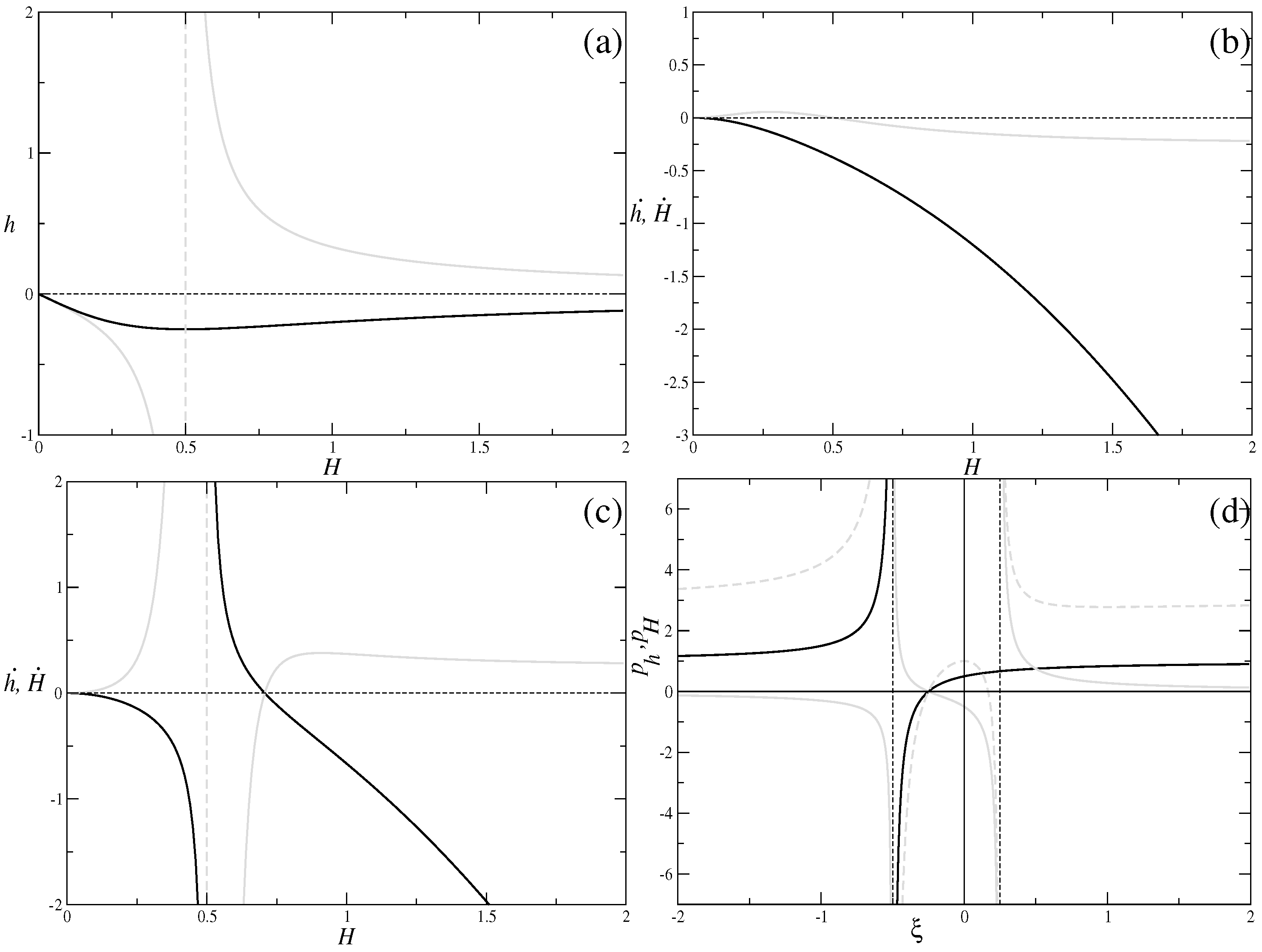
and so H and h have opposite signs for , but could have same sign in the case. We presented them in Figure 1a—black for and grey for . Also, one can resolve Equation (10) for the vacuum case with respect to to obtain
and after that with use of (13) one can solve (9) to get
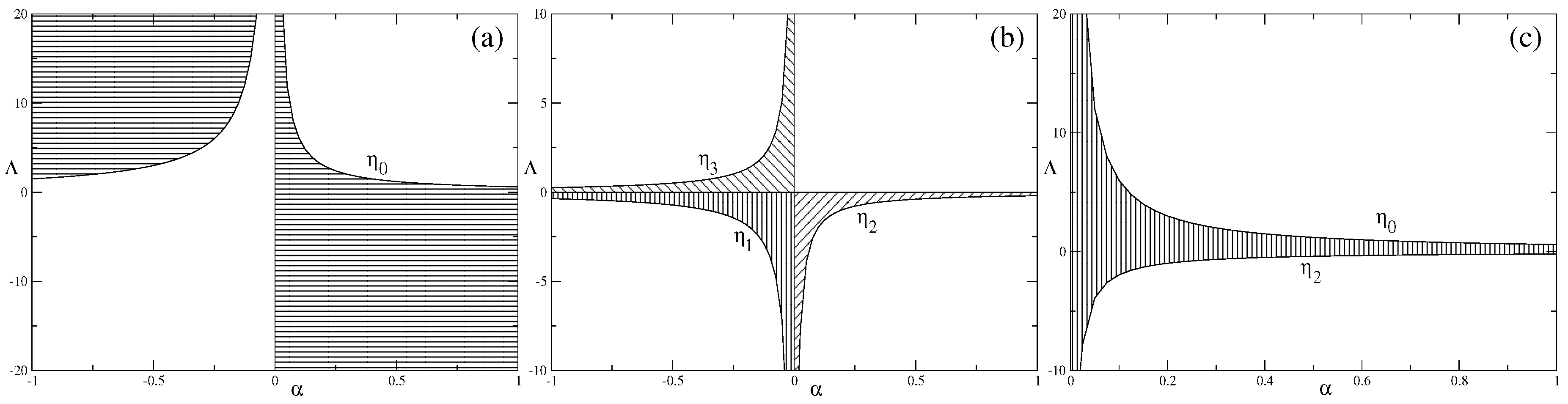
Now we can plot and versus H; these values are depicted in Figure 1b,c. Panel (b) corresponds to the case and panel (c) to ; particular curves correspond to . In these panels we presented in black and in gray.
Finally we can perform analysis in terms of the Kasner exponents ; it is convenient if we want to find power law () asymptotes. With taken from Equations (13)–(14), the Kasner exponents could be easily written down as
We plot the resulting curves in Figure 1d, with represented with a black line, in gray and their sum in dashed gray
Now with all the preliminaries done we can describe regimes. For (black line in Figure 1a, whole Figure 1b, and part of the Figure 1d) we can conclude that there is transition from the power law regime with and , to the low-energy (standard) Kasner regime with ; we shall discuss the notations a bit later.
For (gray line in Figure 1a, whole Figure 1c and part of the Figure 1d) we have three regimes. The first is the high-energy regime transit into the isotropic exponential solution (see [34] for and [19] for ) . at . The second (by decreasing absolute value of H) is the transition from the nonstandard singularity at to the same isotropic exponential solution as above. We comment more on the nonstandard singularities in the Discussion section; here we just mention the situation when or diverges at the final H and/or h, creating physical singularity at final and nonzero H and/or h; we denote these values as . The third regime is the transition from the same nonstandard singularity to low-energy Kasner .
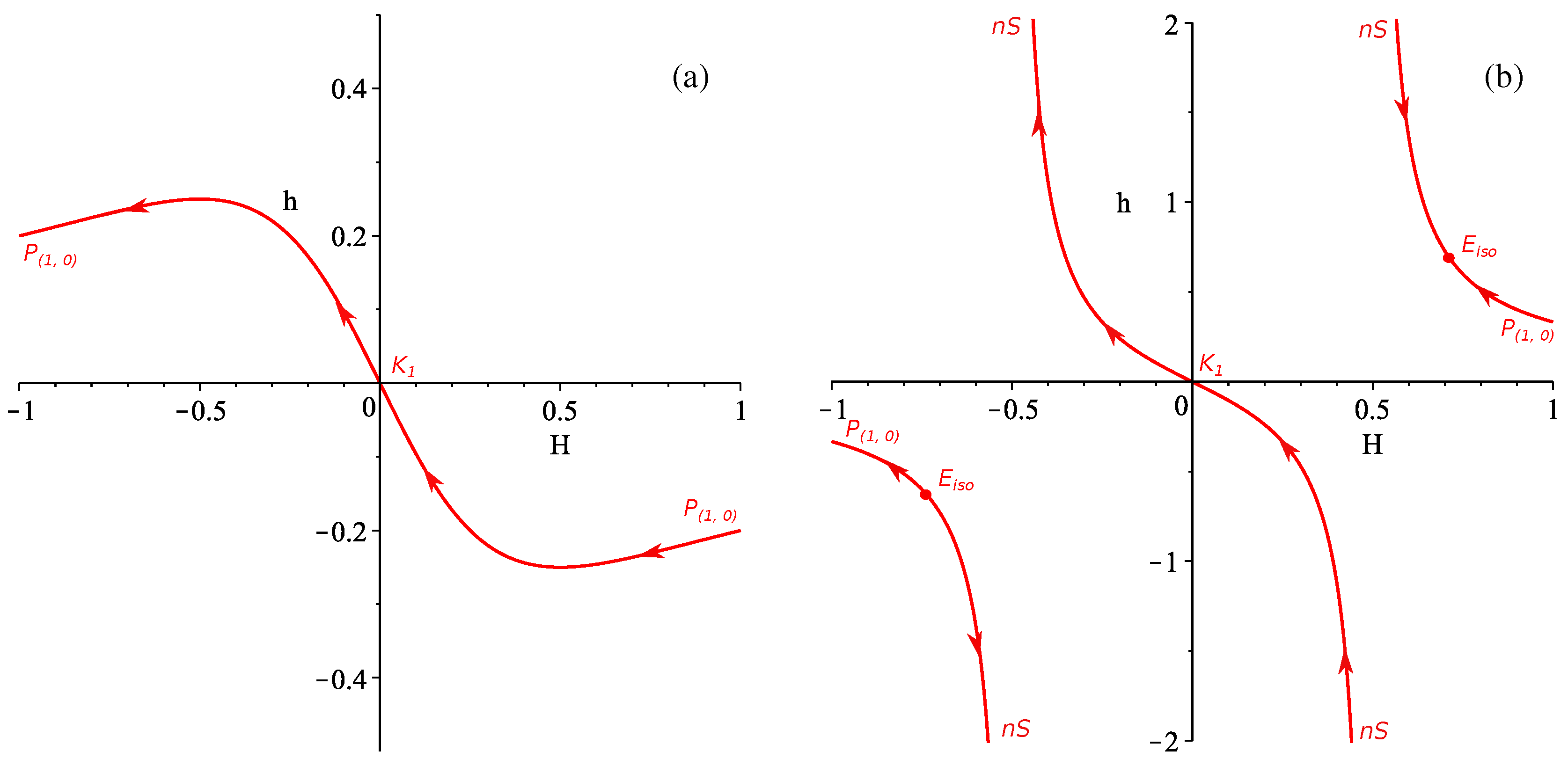
In order to describe all possible regimes for this case—for regardless of the initial —we always have the same transition , so that for all initial , the past asymptote would be , while the future asymptote is . For the situation is different—there are three regimes separated by the isotropic exponential solution at and nonstandard singularity at . Hence, for we have a transition (for all initial the past asymptote would be while the future asymptote is ), for the regime is , and finally for the regime is .
One can see that all possible combinations of and (these are the only independent parameters and are the initial conditions for a well-posed Cauchy problem) fall within the described above four cases, and so give a complete description of the dynamics of this case. For illustrative purposes we combine them in Figure 2— in panel (a) and in panel (b). The direction of the evolution is designed with arrows. In all future cases we shall give the resulting regimes exactly on the (or for high-D cases) graphs.
Now is an appropriate time to introduce and discuss the designations for the regimes we use through the paper. We design exponential solutions with the letter E, with the subindex distinguishing between isotropic () and anisotropic () solutions. The former corresponds to the case where all spatial dimensions expand isotropically; of course this is not what we observe (we observe only three spatial dimensions to expand) so we usually treat as a non-singular yet non-realistic regime. In contrast, is an anisotropic exponential solution with different expansion rates in three and D dimensions (the actual notation is different in each D, for example, in and so on); but to be treated as realistic we require both (the expansion of three-dimensional subspace) and (the extra dimensions that are either constant in size or contract). We added the latter condition to ensure that three dimensions are much larger than the extra dimensions. Of course, this situation is not fulfilled in all , so we comment about it in each particular case.
The power law regimes are a bit tricky. In the original papers [31,32,33] we used only Kasner regimes, but more in-depth investigation revealed that it is not the case and here we provide an updated classification. Hence, there are two classes of power law solution; the first of them is the Kasner solution. As derived in [12], in the Lovelock gravity of the order n, the Kasner solution is defined as and (one can check that the standard Kasner solution with also follows this rule). With that at hand, Gauss–Bonnet Kasner solution should have . However, the solution with and also gives but it is not a Kasner solution (instead it could be seen as generalization of the Taub solution [35]). This misled us in earlier studies [31,32,33] so we have fixed it in current paper. Hence, this is the second class of the power law solutions, which we denote as P with a subindex distinguishing between , () and , (). We discuss the possible connection between this and the Taub solution in the Discussion section.
Finally we denote the nonstandard singularity as —it is a physical singularity which appears in non-linear gravity theories and is due to this non-linearity. We describe and discuss it in the Discussion section; for now we just mention that it is a singular and non-viable regime.
To conclude, in vacuum case there are total four regimes but only two of them are nonsingular— for and for . Of these two only one could be called viable— for —since the other one supposes isotropisation of the entire space and this is not what we observe. Still, the viability of is a big question and we discuss it in the Discussion section.
3.2. Case
The procedure for is generally the same as for ; the difference is in the fact that in the case the constraint is quadratic with respect to h and so instead of a single curve we have two branches. For both of them we repeat the procedure and the results are presented in Figure 3a,b; different colors (red and blue) correspond to different branches. In Figure 3a we present the case, while in Figure 3b . All the regimes are presented there but let us focus only on the realistic ones: for (Figure 3a), and . We see that in we finally have the regular Gauss–Bonnet Kasner solution. The exponential solution , being located in the fourth quadrant of Figure 3a, has and and thus is a viable regime. The same is true for as well—for it we also have and . For (Figure 3b) the only realistic regime is .
To conclude the vacuum case, we finally have a regular Gauss–Bonnet Kasner solution and a viable anisotropic exponential solution ; the list of realistic regimes includes and for and for . Let us also note that in the vacuum case also occurs for .
3.3. Case
This case is also similar to the previous ones and its complexity has also grown a bit—now the constraint equation is cubic with respect to both H and h. Considering that in the general case it is quartic with respect to h and cubic with respect to H, we switch the variable we solve the constraint and for solve it with respect to H. Starting with this case we have three branches for curves; the axes in Figure 3 are also swapped.
The case has an unique feature. Since the number of extra dimensions is three—the same as the number of our spatial dimensions—it is irrelevant which three are expanding and which three are contracting, so we have “double” the number of realistic regimes. Indeed, as we can see from Figure 3c ( case with ), there are two distinct regimes—on the blue branch in the fourth quadrant and on the green branch in the second quadrant. One can see that these are different solutions and they originate from different . The same is true for regimes, which can be found in Figure 3d ( case with ) on the blue branch in the fourth quadrant and on the green branch in the second quadrant. One can also check that they are leading to different and originate from different .
It is interesting to see what becomes of the regime originating from . In , , but in it becomes . Both asymptotes are power law and Taub-like, but the subspaces interchange static and expanding parts—initially one of the subspaces almost is static and another is expanding. Then, the expanding starts to slow down while another starts to expand and finally the initial expansion stops and the initial static expands.
In the vacuum case the situation is similar to the case—we have a realistic regime (actually, two) and for (similar to the case), and a realistic regime for .
3.4. General Case
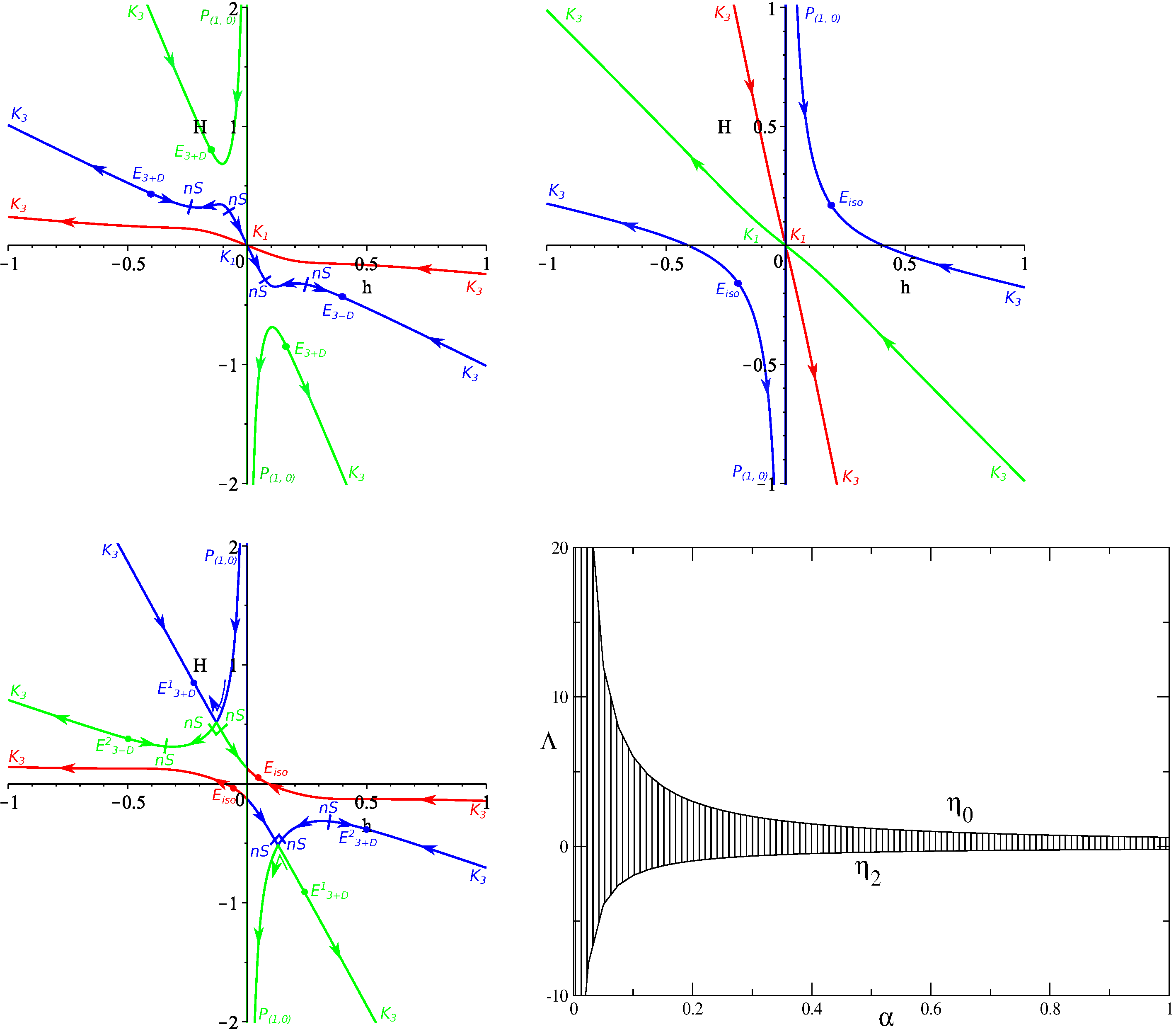
The final case is the general case of . Despite the fact that actual curves are a bit different for each particular D, the shape, derivatives, and so on are quite similar, so we consider the general case with as an example, which can be seen in Figure 3e,f. Similar to the previous cases, the left panel (Figure 3e) is for while the right panel (Figure 3f) is for ; different colors correspond to different branches in the sense of the solutions in the constraint Equation (8) with respect to H.
As we defined the realistic regime as one with and , the regimes vital for us should be located in the second quadrant. One can see that in the fourth quadrant we have the regime which sounds good, but the final anisotropic exponential solution has and . So, despite the fact that the regime is nonsingular, the final state is unrealistic. In the second quadrant of Figure 3e we can see two realistic regimes— and —these regimes correspond to . For , which could be found in Figure 3f, the only realistic regime is from the second quadrant.
To conclude, the general case is similar to the – for it has and regimes (the latter is absent in ) while for it has .
3.5. Conclusions on the Vacuum Case
Overall, the vacuum case demonstrates some consistency over variation of D. In particular, in all D for there is a regime which originates from , but the past asymptote for this regime differs with D. In and it is , in it is and in the general case it is . Apart from these regimes, there are two more which are presented in : for and for .
4. The -Term Case
Now, we consider the -term case. The procedure is exactly the same as in the previous section, but now we have two parameters of the theory (Gauss–Bonnet coupling and the -term). Hence, the classification becomes more complicated and so there are more cases than in the vacuum case.
4.1. The Case
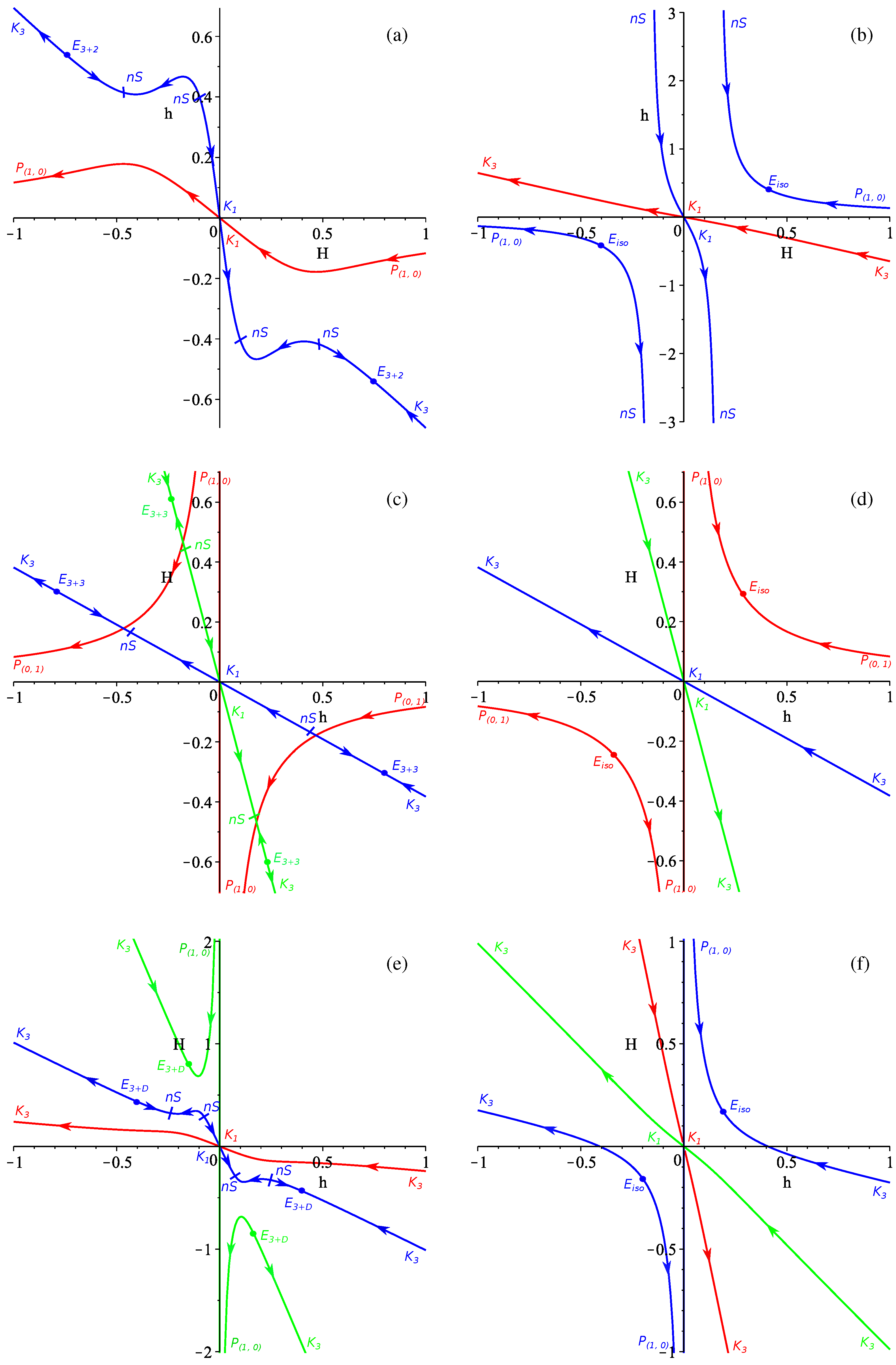
This is the simplest case and, similar to the vacuum case, we have only one branch. The results are presented in Figure 4 and the panel layout is as follows: in panel (a) there is the case; in panel (b) there is the case; in panel (c) ; in panel (d) , in panel (e) and finally in panel (f) we have presented the case.
Analyzing Figure 4 one can see that there is only one regime which could be called viable— —which is present in the fourth quadrant () of Figure 4b (so it is entirely on the subplane). All other regimes either are located in the “wrong” quadrant or have a non-viable past or future asymptote.
Overall, in the -term case we report one possible viable regime——which is the same as in the vacuum case with the difference that now the number of extra dimensions is one. Later in the Discussion section we discuss it more. On comparison with the vacuum case one can note that the dynamics are much richer but the number of realistic regimes is the same—only one.
4.2. The Case
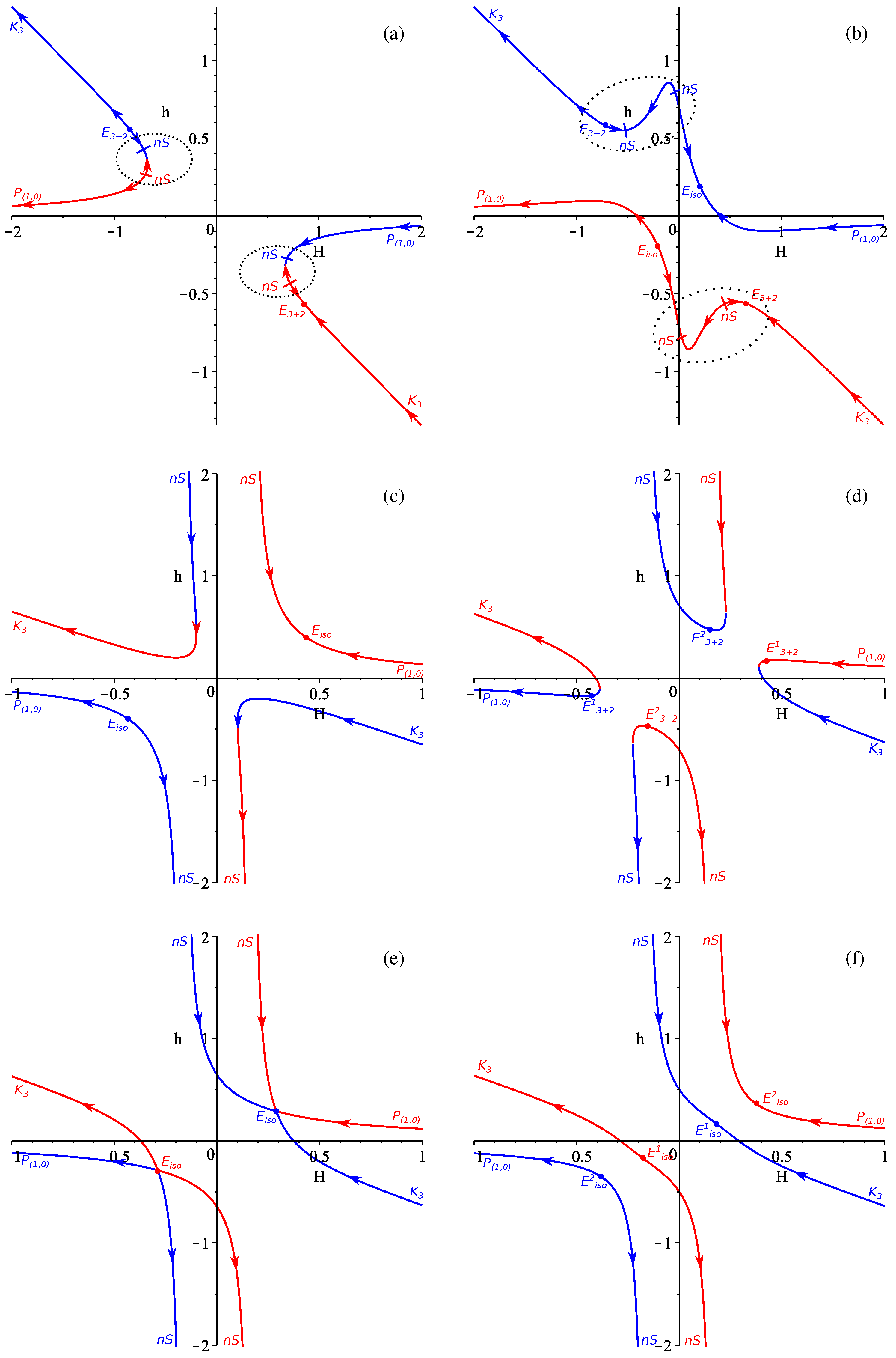
In the -term case, as in the vacuum case, there are two branches and they are represented as different colors in Figure 5. The panel layout is as follows: in panel (a) we presented the case, in panel (b) the case is shown, in panel (c) the case is presented, and the remaining three panels correspond to the cases: in panel (d), in panel (e) and in panel (f).
The first two panels require additional explanations: in Figure 5a we presented case, but there are changes which separate cases with and . As they do not change the shape of the curves, we decided to keep both of them on the same graph. The difference is in addition of two nonstandard singularities for —in Figure 5a they are encircled by a dashed line. For they are absent, and so the regimes for the fourth quadrant () are: . In contrast, for they are present and so the regimes are . This way, the regime , which is realistic, can exist only for .
The second panel which requires additional explanations is Figure 5b. This case corresponds to and there is a fine structure of the anisotropic exponential solutions for (see [32] for details). The particular example of the situation in Figure 5b corresponds to and for other intervals and exact values within the range the abundance and locations of the anisotropic exponential solutions and nonstandard singularities are different (see [32] or Discussions in [33] for details). All of them are “internal” in the sense that they cannot be reached from and they do not introduce new realistic regimes. The regime , which is realistic, exists for ; for it is replaced with .
Of the remaining panels we want to briefly comment on Figure 5d, which corresponds to , . The anisotropic exponential solution is located in the first and third quadrants, but it is so only for . With the decrease of , the location of the solution “moves” towards the axis and for it is located exactly at . For it “moves” even further to on the upper branch and on the bottom. However, since the past asymptotes for the upper branch are both nonstandard singularities, the regime cannot be called viable and we discard it.
The remaining panels do not have realistic regimes so we have only described two in panels (a) and (b): which exists for , and which exists for , (including the entire domain).
Compared with vacuum case, we also have one regime with an anisotropic exponential solution, but lacks power law solutions. In the Discussion section we explain why this is so.
4.3. The Case
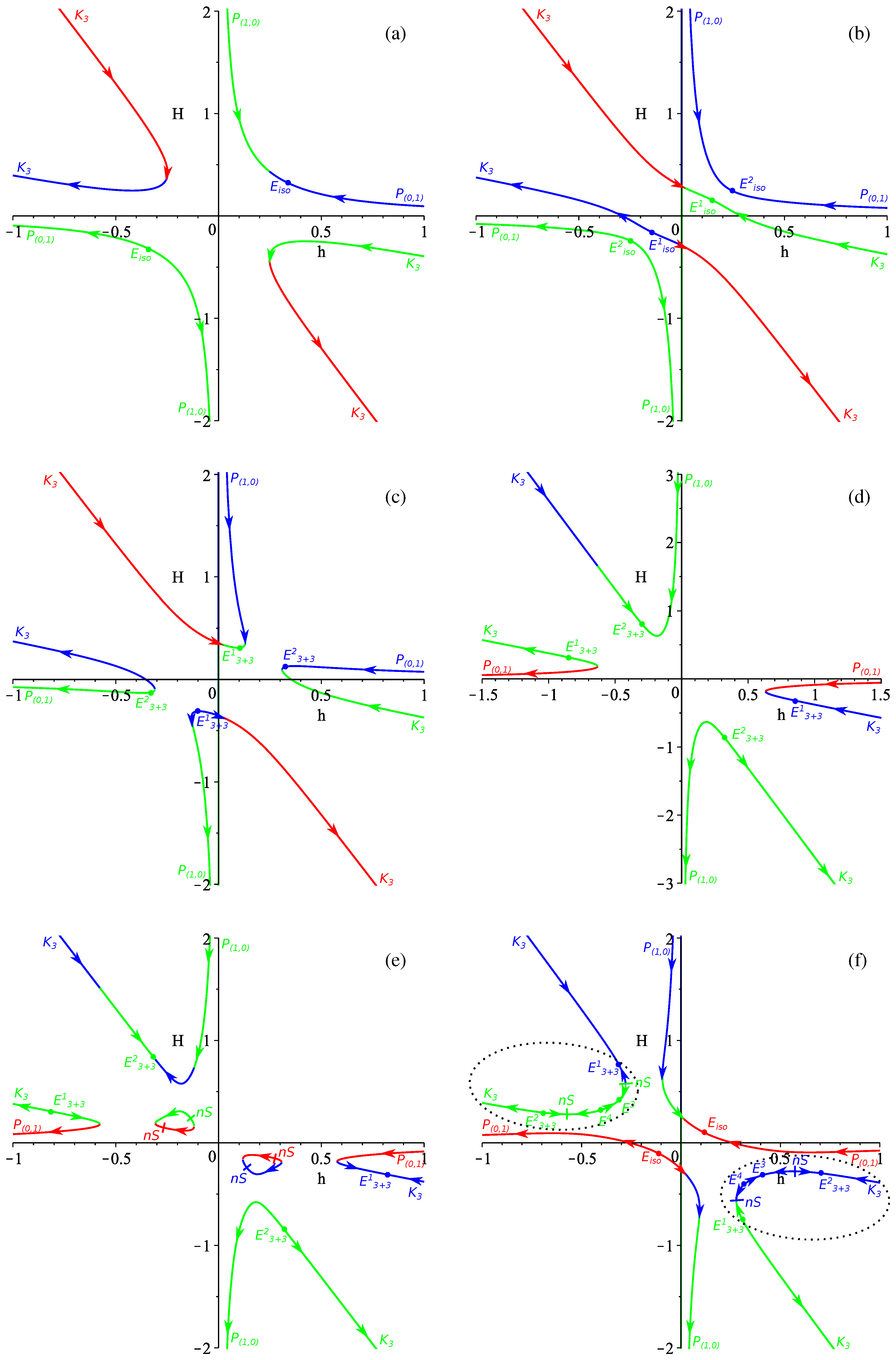
Similar to vacuum case, we have three branches now. Also, as in the vacuum case, both subspaces are three-dimensional, which simplifies the analysis. The results are presented in Figure 6 and the panel layout is as follows: in panel (a) we present the case; in panel (b) the , case is shown; in panel (c) we have the , case; in panel (d), , ; in panel (e) , ; and finally in panel (f) we have the case of . We have not placed here the exact , case, but one can restore it with good precision from Figure 6b by making two isotropic exponential solutions coincide. As in the case of , , the exact case does not have any realistic regimes.
We must comment on the case presented in Figure 6f. Similar to the -term case, described above, there is a fine structure of the anisotropic exponential solutions, which can be found in [33]. However, similar to the mentioned case, the fine structure is “internal” and so changes within do not alter realistic regimes. As in the -term case, there is also the boundary where the realistic regime exists.
Before looking for the remaining realistic regimes, let us note that at , similar to the vacuum case, we solve constraints with respect to H and so swap the axis on the figures; now the realistic regimes () lie in the second quadrant. However, this is also so that only for this case we also can consider ()—the fourth quadrant.
There we can find only a few of the regimes. The interesting regime for is presented in Figure 6a. This is discussed in the Discussion section. In Figure 6c—the , case—the situation is similar to what we described for Figure 5d. The location of is “moving” towards as decreases and at it hits zero (so at anisotropic exponential solution has ). A further decrease of “moves” into the second quadrant for the upper branch and to the fourth quadrant for the lower branch. This way for we have the two realistic regimes and .
The other realistic regimes can be found in Figure 6d (, )—in the second quadrant they are and while in the fourth they are and . Let us note that and are different exponential solutions, but and could be seen as the same. Considering further Figure 6e (, ) one can see that the realistic regimes are exactly the same.
Finally, in the case, presented in Figure 6f, similarly to the previous case we have fine structure of the “internal” anisotropic exponential solutions, which leaves the realistic regime unaffected. This regime exists for —the same value as for the case.
To conclude, there are three potentially realistic regimes in the -term case: for ; for and ; and for and (including the entire domain).
Compared with vacuum case, we have richer dynamics in the -term case.
4.4. General Case
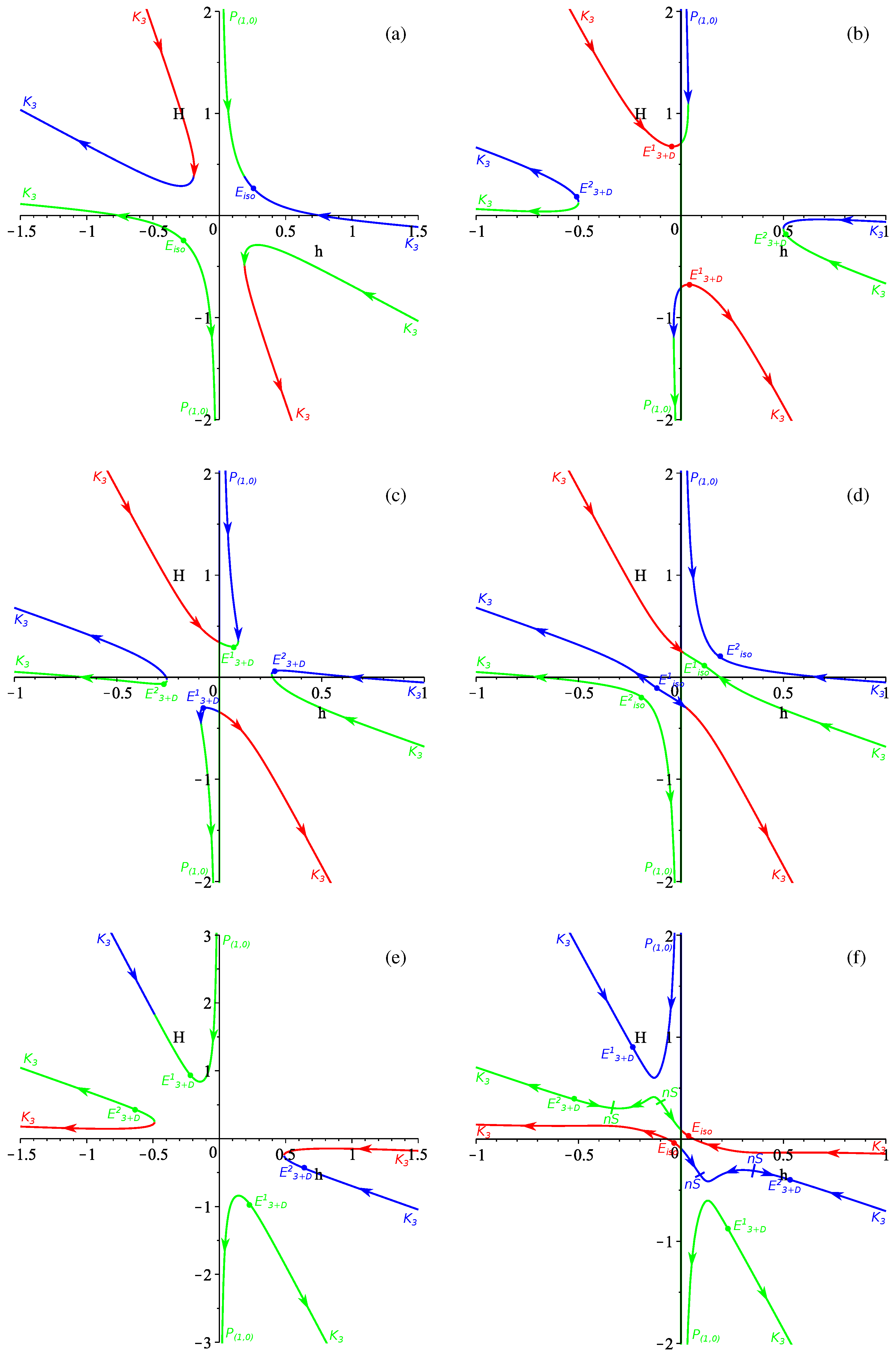
Finally we have the general case. The results are presented in Figure 7 and Figure 8. The panel layout for Figure 7 is as follows: panel (a) corresponds to , panel (b) to , panel (c) to , panel (d) to , panel (e) to and panel (f) to . The panels in Figure 8 are as follows: panel (a) is for while panel (b) is for .
The quoted are exact values found in [33] (where they are denoted as ):
Let us have a look at the resulting regimes and find realistic ones among them; remember that regimes lie in the second quadrant. We have from Figure 7a as a potentially realistic regime. Further, there is and from Figure 7b . This is the “replacement” of the discussed situation “moving” the exponential solution for , which “hits” zero at , but in the general case it hits at . The same realistic regimes— and —can be found in Figure 7e , Figure 7f and Figure 8a . From Figure 8b we can see that only can be called realistic in the case, but, similar to the previous cases, it has the fine structure of anisotropic exponential solutions (see [33] for details) and exists only for where is found in [33] (where it is denoted as ):
To conclude, the general case is quite similar to but the limits are different. We can call the following regimes realistic: for (); and and for and (including the entire domain). For alone the second region is extended to .
Overall, the general -term case demonstrates the richest dynamics of all cases considered so far. It also has the widest areas on the parameters space, which could lead to realistic compactification regimes.
4.5. Conclusions on the -Term Case
To conclude, the richness of the dynamics in different D cases increases with the growth of D, as in the vacuum case. Unlike the vacuum case, where we report almost no changes for all cases, the -term cases have steady growth of the regime abundance with increasing D. In we have only one would-be realistic regime—, which exists for . The situation with changes drastically. This regime is no more but there are two others, and . The former exists for (including the entire domain) while the latter exists for . In we have the additional regime which exists for and two regimes which are the same as in the case, and . They both exist for and ; for the area of existence is extended to . Finally for the general case we have all the regimes from but with partially different areas of existence: has the same area of existence while and exist for and (including the entire domain). For alone the second region is extended to .
5. Discussion
Let us start the discussion of the obtained results with the discussion of the asymptotes. For the past, there are two of them— and . Both of them are power law () regimes, and the difference lies in the expansion rates—for we have and so that and (here stands for the Kasner exponent associated with H while —for h). For it is the opposite situation—for this we have and . Let us note that formally for , and that is why we confused it with in the original papers [31,32,33]; in this paper we clearly separate them. The difference between them is in the expansion rates. For we usually have and , while for it is more “singular-like”— while . We also note that could be treated as a generalized Taub [35] solution. The same is true for , which differs in the swapping of “0” and “1” in the Kasner exponents—for we have (and so asymptotically ) and (and so ). A standard Kasner solution with finalizes the power law regimes presented in the course of study.
There is one important comment on the power law regimes as future asymptotes. In [31,32,33] we noted that , being the future asymptote, is singular and has finite-time future singularity. The same is true for as a future asymptote, at least in the -term case (see [32]). The reason behind it not clear and requires additional investigation, but the fact is stated, and so we remove the regimes with and as future asymptotes from the list of realistic regimes.
With little to comment on with respect to exponential regimes, we turn our attention to another regime which is alien to GR—nonstandard singularity. It can be described as follows: in GR, being linear in the highest derivative, if we solve the dynamical equations with respect to , the resulting expressions are polynomial. On the contrary, for GB and other non-linear theories, the resulting expression is rational function. There could be a situation when the denominator of this function hits zero at some regular H while the numerator is regular and nonzero. In this case the result diverges and so , making this point singular. However, it happens at regular nonzero H, making the situation nonstandard and providing the origin of the name for singularity of this type. Let us note that this kind of singularity is quite common in GB. For the totally anisotropic spatially flat vacuum -dimensional model it is the only future asymptote (see [14]). This kind of singularity is “weak” as per Tipler’s classification [36], and “type II” in classification as per Kitaura and Wheeler [37,38].
We have found domains on the (, ) plane where realistic regimes exist and it is interesting to compare the bounds we have found with those coming from other considerations. The results of this comparison are presented in Figure 9. In Figure 9a we presented the summary of the results from the current paper—, , from (16) in the second quadrant, and , from (18) on the half-plane. In Figure 9b we collected available constraints on from other considerations. Among them a significant number are based on the different aspects of Gauss–Bonnet gravity in AdS spaces—from the consideration of the shear viscosity to entropy ratio as well as causality violations and CFTs in the dual gravity description, limits were obtained on [39,40,41,42,43,44,45,46]:
The limits for dS () are less numerous and are based on different aspects (causality violations, perturbation propagation, and so on) of black hole physics in dS spaces. The most stringent constraint coming from these considerations is [47,48,49]
At this point, two clarifications are required. First, (20) is true for both and , so that in the , quadrant two limits are applied: from (19) and from (20). One can easily check that for so that the constraint from (19) is the most stringent in this quadrant. Secondly, one can see that the limit in (20) is not defined for . Indeed, in this case the limit is special (see [50]), but since for there are no viable cosmological regimes, we consider only.
Secondly, one can see that the bounds on () cover three quadrants and our analysis allows for constraint of the remaining sector: , . However, if we consider joint constraint from Figure 9a,b, the resulting area is presented in Figure 9c. In there, one can see that the regimes in the sector disappear due to the fact that always—the () values, which have viable cosmological dynamics in sector, disagree with (20). To conclude, if we consider our bounds on (, ) together with previously obtained (see (19)–(20)), the resulting bounds are
The result that the joint analysis suggests only , which is interesting and important— indeed, the constraints on () considered so far do not distinguish between , and there are several considerations which favor . The most important of them is the positivity of coming from heterotic string setup, where is associated with inverse string tension [50], but there are several others like ill-definition of the holographic entanglement entropy [51]. Hence, our joint analysis supports as well.
6. Conclusions
In this paper we provide a comprehensive review of the situation of realistic compactification in the spatially flat Einstein–Gauss–Bonnet cosmologies. It is not just a repetition of [31,32,33] but a brand new approach to the problem. The original papers contain a lot of technical details—they are necessary, as they provide proof of the solidness of the results. However, the abundance of the technical details sometimes hides the meaning, and in the present paper we unveil it. We introduce a new presentation of the resulting regimes—placing them all on or curves and indicating the direction of the evolution with arrows. Finally, we corrected ourselves with respect to the wrong treatment of the regime. Our analysis allows us to put constraints on the previously unconstrained sector on the () plane—, . Joint analysis of our bounds on the () with those obtained from other considerations allow us to tighten the constraints on (see Equation (21)) and drop from consideration. However, the field still has a lot of unresolved mysteries, like the mentioned singular behavior of and when they are future asymptotes. We will address this issue in due time.
Conflicts of Interest
The authors declare no conflict of interest.
References
- Nordström, G. Über die Möglichkeit, das Elektromagnetische Feld und das Gravitationsfeld zu vereiningen. Phys. Z. 1914, 15, 504–506. [Google Scholar]
- Nordström, G. Zur Theorie der Gravitation vom Standpunkt des Relativitätsprinzips. Ann. Phys. 1913, 347, 533–554. [Google Scholar] [CrossRef]
- Kaluza, T. Zum Unitätsproblem der Physik. Sit. Preuss. Akad. Wiss. 1921, K1, 966. [Google Scholar]
- Klein, O. Quantentheorie und fünfdimensionale Relativitätstheorie. Z. Phys. 1926, 37, 895–906. [Google Scholar] [CrossRef]
- Klein, O. The Atomicity of Electricity as a Quantum Theory Law. Nature 1926, 118, 516. [Google Scholar] [CrossRef]
- Zwiebach, B. Curvature squared terms and string theories. Phys. Lett. B 1985, 156, 315–317. [Google Scholar] [CrossRef]
- Zumino, B. Gravity theories in more than four dimensions. Phys. Rep. 1986, 137, 109–114. [Google Scholar] [CrossRef]
- Lovelock, D. The Einstein Tensor and Its Generalizations. J. Math. Phys. 1971, 12, 498–501. [Google Scholar] [CrossRef]
- Deruelle, N.; Fariña-Busto, L. Lovelock gravitational field equations in cosmology. Phys. Rev. D 1990, 41, 3696–3708. [Google Scholar] [CrossRef]
- Mu¨ller-Hoissen, F. Dimensionally continued Euler forms: Kaluza-Klein cosmology and dimensional reduction. Class. Quant. Grav. 1986, 3, 665–677. [Google Scholar] [CrossRef]
- Deruelle, N. On the approach to the cosmological singularity in quadratic theories of gravity: The Kasner regimes. Nucl. Phys. B 1989, 327, 253–266. [Google Scholar] [CrossRef]
- Pavluchenko, S.A. General features of Bianchi-I cosmological models in Lovelock gravity. Phys. Rev. D 2009, 80, 107501. [Google Scholar] [CrossRef]
- Pavluchenko, S.A.; Toporensky, A.V. A note on differences between (4 + 1)- and (5 + 1)-dimensional anisotropic cosmology in the presence of the Gauss-Bonnet term. Mod. Phys. Lett. A 2009, 24, 513–521. [Google Scholar] [CrossRef]
- Pavluchenko, S.A. The dynamics of the flat anisotropic models in the Lovelock gravity. I: The even-dimensional case. Phys. Rev. D 2010, 82, 104021. [Google Scholar] [CrossRef]
- Ivashchuk, V. On cosmological-type solutions in multi-dimensional model with Gauss-Bonnet term. Int. J. Geom. Meth. Mod. Phys. 2010, 07, 797–819. [Google Scholar] [CrossRef]
- Kirnos, I.V.; Makarenko, A.N.; Pavluchenko, S.A.; Toporensky, A.V. The nature of singularity in multidimensional anisotropic Gauss-Bonnet cosmology with a perfect fluid. Gen. Rel. Grav. 2010, 42, 2633–2641. [Google Scholar] [CrossRef]
- Pavluchenko, S.A.; Toporensky, A.V. Note on properties of exact cosmological solutions in Lovelock gravity. Gravit. Cosmol. 2014, 20, 127–131. [Google Scholar] [CrossRef]
- Kirnos, I.V.; Pavluchenko, S.A.; Toporensky, A.V. New features of flat (4+1)-dimensional cosmological model with a perfect fluid in Gauss-Bonnet gravity. Gravit. Cosmol. 2010, 16, 274–282. [Google Scholar] [CrossRef]
- Chirkov, D.; Pavluchenko, S.; Toporensky, A. Exact exponential solutions in Einstein-Gauss-Bonnet flat anisotropic cosmology. Mod. Phys. Lett. A 2014, 29, 1450093. [Google Scholar] [CrossRef]
- Chirkov, D.; Pavluchenko, S.; Toporensky, A. Constant volume exponential solutions in Einstein-Gauss-Bonnet flat anisotropic cosmology with a perfect fluid. Gen. Rel. Grav. 2014, 46, 1799. [Google Scholar] [CrossRef]
- Chirkov, D.; Pavluchenko, S.; Toporensky, A. Non-constant volume exponential solutions in higher-dimensional Lovelock cosmologies. Gen. Rel. Grav. 2015, 47, 137. [Google Scholar]
- Pavluchenko, S.A. Stability analysis of the exponential solutions in Lovelock cosmologies. Phys. Rev. D 2015, 92, 104017. [Google Scholar] [CrossRef]
- Ivashchuk, V.D. On stability of exponential cosmological solutions with nonstatic volume factor in the Einstein-Gauss-Bonnet model. Eur. Phys. J. C 2016, 76, 431. [Google Scholar] [CrossRef]
- Ivashchuk, V.D.; Kobtsev, A.A. Stable exponential cosmological solutions with 3- and l-dimensional factor spaces in the Einstein-Gauss-Bonnet model with a Λ-term. Eur. Phys. J. C 2018, 78, 100. [Google Scholar] [CrossRef]
- Canfora, F.; Giacomini, A.; Pavluchenko, S.A. Dynamical compactification in Einstein-Gauss-Bonnet gravity from geometric frustration. Phys. Rev. D 2013, 88, 064044. [Google Scholar] [CrossRef]
- Canfora, F.; Giacomini, A.; Pavluchenko, S.A. Cosmological dynamics in higher-dimensional Einstein-Gauss- Bonnet gravity. Gen. Rel. Grav. 2014, 46, 1805. [Google Scholar] [CrossRef]
- Canfora, F.; Giacomini, A.; Pavluchenko, S.A.; Toporensky, A. Friedmann dynamics recovered from compactified Einstein-Gauss-Bonnet cosmology. Gravit. Cosmol. 2018; arXiv:1605.00041. [Google Scholar]
- Pavluchenko, S.A. The generality of inflation in closed cosmological models with some quintessence potentials. Phys. Rev. D 2003, 67, 103518. [Google Scholar] [CrossRef]
- Pavluchenko, S.A. Constraints on inflation in closed universe. Phys. Rev. D 2004, 69, 021301. [Google Scholar] [CrossRef]
- Pavluchenko, S.; Toporensky, A. Effects of spatial curvature and anisotropy on the asymptotic regimes in Einstein-Gauss-Bonnet gravity. arXiv, 2017; arXiv:1709.04258. [Google Scholar]
- Pavluchenko, S.A. Cosmological dynamics of spatially flat Einstein-Gauss-Bonnet models in various dimensions. Vacuum case. Phys. Rev. D 2016, 94, 024046. [Google Scholar] [CrossRef]
- Pavluchenko, S.A. Cosmological dynamics of spatially flat Einstein-Gauss-Bonnet models in various dimensions: Low-dimensional Λ-term case. Phys. Rev. D 2016, 94, 084019. [Google Scholar] [CrossRef]
- Pavluchenko, S.A. Cosmological dynamics of spatially flat Einstein-Gauss-Bonnet models in various dimensions: High-dimensional Λ-term case. Eur. Phys. J. C 2017, 77, 503. [Google Scholar] [CrossRef]
- Ivashchuk, V.D. On anisotropic Gauss-Bonnet cosmologies in (n+1) dimensions, governed by an n-dimensional Finslerian 4-metric. Grav. Cosmol. 2010, 16, 118–125. [Google Scholar] [CrossRef]
- Taub, A.H. Empty Space-Times Admitting a Three Parameter Group of Motions. Ann. Math. 1951, 53, 472–490. [Google Scholar] [CrossRef]
- Tipler, F.J. Singularities in conformally flat spacetimes. Phys. Lett. A 1977, 64, 8–10. [Google Scholar] [CrossRef]
- Kitaura, T.; Wheeler, J.T. Anisotropic, time-dependent solutions in maximally Gauss-Bonnet extended gravity. Nucl. Phys. B 1991, 355, 250–277. [Google Scholar] [CrossRef]
- Kitaura, T.; Wheeler, J.T. New singularity in anisotropic, time-dependent, maximally Gauss-Bonnet extended gravity. Phys. Rev. D 1993, 48, 667–672. [Google Scholar] [CrossRef]
- Brigante, M.; Liu, H.; Myers, R.C.; Shenker, S.; Yaida, S. Viscosity Bound Violation in Higher Derivative Gravity. Phys. Rev. D 2008, 77, 126006. [Google Scholar]
- Brigante, M.; Liu, H.; Myers, R.C.; Shenker, S.; Yaida, S. Viscosity Bound and Causality Violation. Phys. Rev. Lett. 2008, 100, 191601. [Google Scholar]
- Buchel, A.; Myers, R.C. Causality of Holographic Hydrodynamics. JHEP 2008, 0908, 016. [Google Scholar] [CrossRef]
- Hofman, D.M. Higher Derivative Gravity, Causality and Positivity of Energy in a UV complete QFT. Nucl. Phys. B 2009, 823, 174–194. [Google Scholar] [CrossRef]
- De Boer, J.; Kulaxizi, M.; Parnachev, A. AdS_7/CFT_6, Gauss-Bonnet Gravity, and Viscosity Bound. JHEP 2010, 1003, 087. [Google Scholar] [CrossRef]
- Camanho, X.O.; Edelstein, J.D. Causality constraints in AdS/CFT from conformal collider physics and Gauss-Bonnet gravity. JHEP 2010, 1004, 007. [Google Scholar] [CrossRef]
- Buchel, A.; Escobedo, J.; Myers, R.C.; Paulos, M.F.; Sinha, A.; Smolkin, M. Holographic GB gravity in arbitrary dimensions. JHEP 2010, 1003, 111. [Google Scholar]
- Ge, X.-H.; Sin, S.-J. Shear viscosity, instability and the upper bound of the Gauss-Bonnet coupling constant. JHEP 2009, 0905, 051. [Google Scholar] [CrossRef]
- Cai, R.G.; Guo, Q. Gauss-Bonnet black holes in dS spaces. Phys. Rev. D 2004, 69, 104025. [Google Scholar] [CrossRef]
- Cai, R.G. Gauss-Bonnet black holes in AdS spaces. Phys. Rev. D 2002, 65, 084014. [Google Scholar] [CrossRef]
- Cai, R.G. A note on thermodynamics of black holes in Lovelock gravity. Phys. Lett. B 2004, 582, 237–242. [Google Scholar] [CrossRef]
- Boulware, D.G.; Deser, S. String-generated gravity models. Phys. Rev. Lett. 1985, 55, 2656–2660. [Google Scholar] [CrossRef] [PubMed]
- Ogawa, N.; Takayanagi, T. Higher Derivative Corrections to Holographic Entanglement Entropy for AdS Solitons. JHEP 2011, 1110, 147. [Google Scholar] [CrossRef]
Figure 1.
Graphs illustrating the dynamics of the vacuum cosmological model. In panel (a) we present the behavior for from (12). Black is used for and gray for . In panels (b) and (c) we present in black and in gray for (panel (b)) and (panel (c)). Finally, in panel (d) we present the Kasner exponents in black, in gray, and the expansion rate in dashed gray; irregularities are denoted as dashed black lines (see the text for more details).

Figure 2.
(a,b) The regimes shown in the resulting graph for the vacuum case (see the text for more details).
Figure 2.
(a,b) The regimes shown in the resulting graph for the vacuum case (see the text for more details).

Figure 3.
The regimes shown in the resulting graph for the vacuum case (panels (a,b)), the vacuum case (panels (c,d)), and the general case (panels (e,f)) (see the text for more details).
Figure 3.
The regimes shown in the resulting graph for the vacuum case (panels (a,b)), the vacuum case (panels (c,d)), and the general case (panels (e,f)) (see the text for more details).

Figure 4.
(a–f) The regimes shown in the resulting graph for the -term case (see the text for more details).
Figure 4.
(a–f) The regimes shown in the resulting graph for the -term case (see the text for more details).

Figure 5.
(a–f) The regimes shown in the resulting graph for the -term case (see the text for more details).
Figure 5.
(a–f) The regimes shown in the resulting graph for the -term case (see the text for more details).

Figure 6.
(a–f) The regimes shown in the resulting graph for the -term case (see the text for more details).
Figure 6.
(a–f) The regimes shown in the resulting graph for the -term case (see the text for more details).

Figure 7.
(a–f) The regimes shown in the resulting graph for the -term case (see the text for more details).
Figure 7.
(a–f) The regimes shown in the resulting graph for the -term case (see the text for more details).

Figure 8.
(a,b) Additional regimes shown in the resulting graph for the -term case (see the text for more details).
Figure 8.
(a,b) Additional regimes shown in the resulting graph for the -term case (see the text for more details).
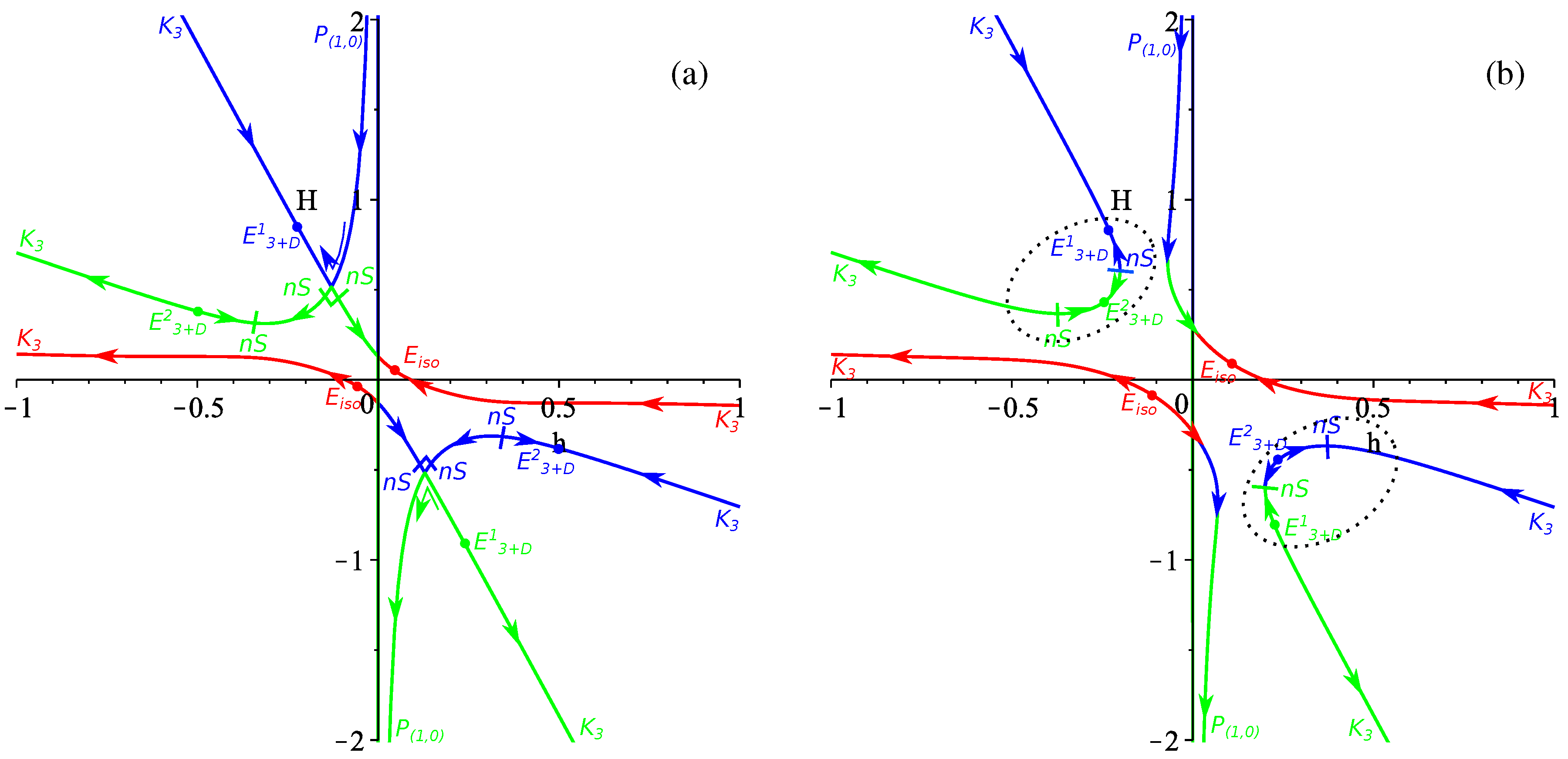
Figure 9.
Summary of the bounds on () from this paper alone in panel (a); from other considerations found in the literature in panel (b); and the intersection between them in panel (c) (see the text for more details).
Figure 9.
Summary of the bounds on () from this paper alone in panel (a); from other considerations found in the literature in panel (b); and the intersection between them in panel (c) (see the text for more details).

© 2018 by the author. Licensee MDPI, Basel, Switzerland. This article is an open access article distributed under the terms and conditions of the Creative Commons Attribution (CC BY) license (http://creativecommons.org/licenses/by/4.0/).
Share and Cite
MDPI and ACS Style
Pavluchenko, S. Realistic Compactification Models in Einstein–Gauss–Bonnet Gravity. Particles 2018, 1, 36-55. https://doi.org/10.3390/particles1010004
AMA Style
Pavluchenko S. Realistic Compactification Models in Einstein–Gauss–Bonnet Gravity. Particles. 2018; 1(1):36-55. https://doi.org/10.3390/particles1010004
Chicago/Turabian StylePavluchenko, Sergey. 2018. "Realistic Compactification Models in Einstein–Gauss–Bonnet Gravity" Particles 1, no. 1: 36-55. https://doi.org/10.3390/particles1010004