Stochastic Stability of a Class of MEMS-Based Vibratory Gyroscopes under Input Rate Fluctuations

Department of Mechanical and Materials Engineering, The University of Western Ontario, London, ON N6A 5B9, Canada
*
Author to whom correspondence should be addressed.
Vibration 2018, 1(1), 69-80; https://doi.org/10.3390/vibration1010006
Submission received: 18 May 2018
/
Revised: 14 June 2018
/
Accepted: 16 June 2018
/
Published: 19 June 2018
Abstract
:The influence of stochastic fluctuations in the input angular rate of a class of single axis mass-spring microelectromechanical (MEM) gyroscopes on the system stability is investigated. A white noise fluctuation is introduced in the coupled 2-DOF model that represents the system dynamics for the purposes of stability prediction. Numerical simulations are performed employing the resulting set of stochastic differential equations (SDEs) that govern the system dynamics. The SDEs are discretized using the higher-order Milstein scheme for numerical computations. Simulations via the Euler scheme, as well as the measure of the largest Lyapunov exponent are employed for validation purposes due to a lack of similar analytical solutions or experimental data. Responses have been predicted under different noise fluctuation magnitudes and different input angular rates for stability investigations. A parametric study is performed to estimate the noise intensity stability threshold for a range of quality factor values at different input angular rates. The predicted results show a nonlinear dependence of the threshold on the quality factors for different input rates. Under typical gyroscope operating conditions, a realistic frequency mismatch appears to have insignificant influence on system stability. It is envisaged that the present quantitative predictions will aid improvements in performance, reliability, and the design process for this class of devices.
1. Introduction
Numerous emerging applications use a micro-machined angular rate sensor or gyroscope as a stand-alone unit or as part of an inertial measurement unit (IMU). In particular, traction control systems, ride stabilization, and rollover detection in automotive applications currently use the micro-machined angular rate gyroscopes. Many other applications, such as digital video camera stabilization systems, missile guidance systems, and platform stabilization systems take advantage of using this class of device (see, e.g., [1]). The low manufacturing cost, moderate performance, and miniature nature of these gyroscopes are the reasons behind their acceptance in these applications [2]. The accuracy of this class of devices is likely to be influenced by a number of sources, including a combination of temperature, vibration, acoustic, shock, thermal cycling, and humidity [1]. For instance, microelectromechanical systems (MEMS) devices can be exposed to shock during fabrication, deployment and operation [3], as well as vibratory excitation resulting from the environment. The undesirable sources can change the dynamic behavior of MEMS devices and, hence, affect their performance. For example, vibratory gyroscopic systems in automotive applications are susceptible to environmental vibrations due to road unevenness and due to other sources. The excitation from road irregularity is modeled as a stationary random process with road roughness suggested in the ISO standard. Furthermore, white noise is often used to model the input of road displacement excitation (see, e.g., [4]). An approximate modeling of rail track unevenness and road irregularities using a white noise excitation is also reported in the prediction of the random vibration response of rail and land vehicles [5]. Aerospace, marine, and other applications are expected to benefit from developments in this class of MEMS gyroscopes. In such applications, the effects of noise and vibration, which stem from the aerodynamic/wave environment, as well as combustion process in propellers, need to be investigated in detail.
MEMS-based gyroscopes, at present, are considered as low-accuracy rate-grade sensors compared to the tactical and inertial-grade sensors which are known to have moderate to high accuracies. However, MEMS-based gyroscopes offer cost and size advantages compared to the tactical and inertial grade counterparts. Thus, to enhance the accuracy of MEMS-based gyroscopes to that of a tactical or inertial grade, further improvements in accuracy, as well as their drift performance, are warranted. To this end, several recent studies, as well as development efforts, are underway. Micro-machined gyroscopes have different design and sensing principles, but almost all the configurations utilize the transfer of energy between two vibration modes of a structure where the Coriolis’ effect is exploited for the precise sensing of angular rotation rates. These devices, in contrast to the conventional gyroscopes, do not contain rotating elements; thus, they are suitable for batch micro fabrication and miniaturization. An external vibratory excitation is used in this class of MEMS device for their operation, but few designs take advantage of parametric excitation (see, e.g., [6,7]).
In order to achieve further improvement and development of this class of sensors, dynamics and stability of this type of gyroscopes have been of interest in the recent past. Mechanical coupling between the drive and detection modes of a single mass-spring micro-machined vibratory gyroscope was studied by Mochida et al. [8] giving importance to the mechanical coupling, then reducing the coupling via the introduction of new designs and fabrication structures [8]. A precise mathematical model for a dual-axis gyroscope was developed by Davis [9], and linear and non-linear suspensions have been considered in this study. This gyroscope was fabricated in the laboratory, but required further investigation prior to commercialization. In the same study, a more accurate model for the single-mass spring gyroscope considering the coupling effect for both the driving and sensing axes has been developed. However, in all of the above studies, instability investigations were not performed. The effect of stochastic fluctuations in the input angular rate on the stability of a single-axis mass-spring vibratory gyroscope has been investigated by Asokanthan and Wang [10]. An approximate analytical method based on the stochastic averaging procedure has been employed to investigate the stability of a vibratory MEMS gyroscope system. Closed-form conditions for mean-square stability of the dynamic response are obtained for the case of exponentially correlated noise. It may be noted that this study focussed only on narrow band frequency ranges that correspond to certain multiples and combinations of system natural frequencies, and predictions for white-noise fluctuations were not presented. Recently, a simplified two degree-of-freedom dynamic model of a ring-based gyroscope is employed to identify the stability of the system when the input angular speed is exposed to random fluctuations [11]. The system response is numerically predicted when the input angular rate is subjected to a white noise fluctuation using the higher-order Milstein scheme that discretizes the governing stochastic differential equations (SDEs). The stability threshold values for noise intensity have been identified using largest Lyapunov exponents’ measure for various damping values. The current study focuses on the stability of the single axis mass-spring gyroscope subjected to stochastic angular speed fluctuation. It is known that use of white noise in the stability investigations presents a more practical representation of the speed fluctuation generated by the environment when compared to the consideration of harmonic vibration or narrow band noise. Thus, the introduction of white noise is expected to predict a more accurate dynamic response of these devices, as well as the physical systems they are mounted on. Hence, the effect of wide-band random fluctuation in the input angular rate on the dynamic stability of the single axis mass-spring structure gyroscope is the main interest of the present study.
Owing to the fact that obtaining a closed-form analytical solution for a multi-dimensional system of stochastic differential equations is cumbersome due to their highly non-differentiable character of the realization of the Wiener process [12], a number of iterative approaches to integrate SDE’s numerically have been developed in the recent past. The most widely used methods are Euler–Maruyama, Euler–Heun, Milstein, derivative-free Milstein (Runge–Kutta approach), and stochastic Runge–Kutta [13]. In the present study, the higher-order Milstein scheme is employed to simulate the time response so that the stochastic response of a single axis mass-spring rate gyroscopes can be quantified for certain parameters of interest. Based on the obtained responses, the behavior of the dynamical system is analyzed. To this end, the characteristic Lyapunov exponents of the stochastic response is evaluated to determine the stability thresholds. The effects of quality factors and the magnitude of the angular speed fluctuation, as well as the frequency mismatch on system stability have been quantified.
2. Governing Equations
The single axis mass-spring rate gyroscope model used in the present study is based on the model developed by Davis [9] and later presented in the work by Asokanthan and Wang [10]. The developed governing equations for the gyroscopic system is employed to investigate the stochastic fluctuation of the input angular rate. The gyroscope configuration consists of a lumped point mass (proof mass) at the center and four springs that support the mass as shown in Figure 1 with dissipating linear viscous damping. As a gyroscope, the mass is excited along the driving x-direction (also referred to as the driving direction), by an external periodic force where the excitation frequency is chosen close to the natural frequency of the system. The gyroscopic system is subjected to an input angular rate Ω about the z-axis where Ω represents the quantity to be measured. The mass is constrained to oscillate in the x–y plane. Thus, a rotation rate, Ω, about the z-axis induces an oscillatory Coriolis force in the y-axis direction (also referred to as the sensing axis). The y-axis oscillatory motion is sensed and used as a basis for the measurement of the angular rate.
The system of coupled second-order differential equations that governs the motion of the gyroscope derived by Davis [9] is presented as follows:
where represents the proof mass. The coefficients and denote the viscous damping constants in the x- and y-directions, respectively, while and are the spring constants in the x- and y-directions, respectively. Additionally, the gyroscope angular rate measurement about the z-direction is denoted by . The main interest of this work is on examining the effects of some important parameters on the system stability. Hence, the steady state part of the response does not play a role. To this end, consideration of the homogenous part of the equations of motion in the absence of the excitation force is adequate. Equation (1) can then be written in matrix form:
with , , , and . The vector represents the vector of the system generalized coordinates, i.e.,, while and , respectively, are the undamped natural frequencies associated with the x- and y-directions. The quality factors representing damping in the x and y directions are denoted by and , respectively. The quality factor is a dimensionless parameter that indicates the energy losses within a resonant element. In general, energy dissipation in vibratory MEMS is governed by several mechanisms, including viscous damping, dissipation through the substrate, thermo-elastic dissipation, and resonator surface effects [14]. The quality factor indicates energy loss relative to the amount of energy stored within the system. Thus, the higher the quality factor the lower the rate of energy loss and, hence, oscillations will decay more slowly. It may be noted that the stiffness matrix includes the centrifugal force term , which takes a negative value for the present system. Hence, overall system stiffness decreases with higher angular velocity that may lead to lower system stability. The damping matrix, apart from representing viscous dissipation, includes the gyroscopic coupling term , which is dependent on the input angular velocity. Moreover, for a constant angular rate, the term . This case is not practical in the presence of fluctuations in the angular rate. However, for the system under investigation, the contributions of the associated terms, and , are considered negligible when compared to the gyroscopic terms and at high angular rates where instability becomes an issue, it is sufficient to approximate for the purpose of stability analysis. Implications and limitations due to this assumption are highlighted in the Results and Discussion section.
The numerical schemes to be used in the present study require the system equations to be transformed to a set of first-order stochastic differential equation in incremental form. For this purpose, Equation (1) is first transformed into a system of four first-order differential equations to accommodate these methods. A set of four state variables is defined as , , , and , and the random fluctuation in the input angular rate is then incorporated in the system to form the governing equations of motion in the standard first-order SDE form. Equation (1) is written in state-space form as:
The random fluctuations in the input angular velocity are assumed to be represented by a white noise process. A Brownian motion function is employed for this purpose to simulate the random fluctuations taking advantage of its first-time derivatives as Gaussian white noise (see, e.g., [15]). Introducing white noise,, with a noise intensity magnitude, , to the nominal input angular velocity,, for representing the random fluctuations, the input angular velocity is written as:
The centrifugal component in the equations of motion which are governed by the terms in Equations (3) can be evaluated using Equation (4) as:
since the random fluctuation term,, is considered small relative to the nominal angular rate, , the last term in Equation (5), , is negligible due to its lower-order of smallness. In addition, for the purposes of simulations, a noise intensity ratio,, is introduced to characterize the noise intensity magnitude, , as:
Combining (Equations (3)–(5)), a system of standard SDEs that represents the gyroscope motion is obtained as:
where the vectors and , respectively, are known as the drift and the diffusion vectors (see, e.g., [12,15]). For the present system, the vector elements written in terms of the state vector are given by:
3. Numerical Simulation Scheme
It is known that obtaining analytical solutions of the standard first-order stochastic differential equations, which govern the gyroscope motion and were formulated in Section 2, is cumbersome, the present study attempts to employ numerical solutions of such systems. To this end, the discretization of SDE using Itô–Taylor expansion, which leads to the higher-order Milstein scheme [16], is employed. The Milstein scheme is a numerical scheme for solving stochastic deferential equations with a strong order of convergence. The method uses Itô’s lemma to increase the accuracy of the approximation by adding the second-order term to approximate numerical solution of a stochastic differential equation. In this technique, the sequence of values of the Milstein approximation at the instants of the time discretization can be computed in a similar way to those of the deterministic case. The main difference is that we now need to generate the random increments of the Wiener process. For a given time discretization, the Milstein scheme determines values of the approximating process at the discretization times only. In order to clarify the approach, the following first-order standard SDE for a scalar dependent variable is used:
along with an Itô–Taylor expansion, where and , respectively, denote the drift and the diffusion terms while represents the driving Wiener process. Use of Itô’s Lemma leads to:
where:
When Itô’s Lemma is iterated to obtain constant integrands for the higher order terms, and assuming that and are not direct functions of , the integrated form of Equation (9) becomes:
where represents terms that include , or terms of higher order, and denotes the derivative with respect to variable . This equation forms the theoretical basis for both Euler and Milstein schemes [16]. It may be noted that the Euler scheme is constructed using the first three terms of this expansion, while incorporation of the fourth term yields the Milstein scheme.
Considering the time interval by choosing , , the discretized form of the Milstein method is formulated as:
Equation (11), when extended to multi-dimensional systems, yields the component of the state vector employing the Milstein scheme for numerical computations and takes the general form:
where the drift and diffusion terms, the driving Wiener process and the variables, are written in vector form. In Equation (12):
where is the diffusion coefficient matrix, is the number of dimensions, and represents the number of independent Weiner processes [15]. In the special case when , the following integral is obtained:
The vector-based scheme presented in Equation (12), considering the system drift and diffusion coefficient matrices, is employed for the purposes of performing numerical computations to solve the system of equations that govern the gyroscope response. To this end, considering Equation (7) and setting to 4 and to 1 in Equation (12), the response takes the form:
The resulting four equations are employed in the prediction of the gyroscope response.
4. Results and Discussion
In the present numerical study, a smooth increase of the input angular rate from zero to different practical values is employed for the purposes of response predictions considering a noise intensity ratio as defined in Equation (6). For the purposes of numerical simulations, the parameters of the single-axis gyro parameters as shown in Table 1 have been used.
Conforming to the goal of the present study, namely the stability investigation, the time response of the gyroscope when subjected to appropriate initial disturbance is examined. In the simulations, an initial displacement of the driving coordinate, , is imposed with a value of and the displacement of sensing coordinate is then computed to evaluate the gyroscope response. However, for high quality factors, which are typical in this class of devices, the convergence of the Milstein scheme is very slow even for a deterministic system. In order to accelerate the convergence, the first two terms in Equation (13) which represent the deterministic part of the numerical solution are evaluated using a fourth-order Runge–Kutta scheme and the values at each time step are used in each iteration for obtaining the complete solution incorporating random terms.
The convergence of the simulation algorithm has been tested for many quality factors, and ranging from to for different relative noise intensity ratio values in the range of to in order to guarantee the accuracy, as well as the appropriateness, of the schemes. Very good convergence has been reached for a time step of ; however, is used for more accuracy and a simulation time of is chosen for the simulations, which are adequate for the remainder of the study. The higher-order Milstein scheme is known to achieve higher accuracy compared to the Euler method; therefore, the first approach is chosen in the present investigations for stability predictions. Time responses of the two methods for the purposes of verifying the response predictions are generated and depicted in Figure 2, Figure 3 and Figure 4. The figures show the responses of the gyroscope at different fluctuation magnitudes in input angular rate at demonstrating various stability behaviors. Maximum relative noise intensity, as defined in Equation (6) has been used as a magnitude measure for representing environment fluctuation. In Figure 2, the system response for quality factor of 500 and maximum relative noise intensity measure demonstrates a stable behavior for this sufficient level of damping. Increasing the noise intensity to a sufficiently high value to cause a noticeable disturbance in the system, along with high enough quality factors that do not suppress the oscillation, causes oscillatory motion as shown in Figure 3. It may be noted that a certain threshold intensity measure for each quality factor is associated with the transition to instability and this measure can be computed using the time responses. Thus, crossing this threshold with a high quality factor or, alternatively, with higher noise intensity, leads to system instability, as shown in Figure 4.
Further, it may be noted that the predicted responses from the Euler and Milstein schemes are similar with slightly larger amplitude values for Milstein than the values predicted by the Euler scheme, which does not take the higher-order terms into account. Thus, the Euler scheme produces an under-predicted response and exhibits increased system stability compared to the Milstein scheme predictions. Accordingly, under certain conditions of noise intensity values, which are close to the threshold, a stable system behavior is predicted via the Euler scheme while an unstable system behavior is predicted by the Milstein scheme, as depicted in Figure 5. Therefore, due to a lack of any exact analytical or experimental results to verify the acquired data against, the accuracy of the employed model should be assessed before performing the parameter sweep which includes varying the relevant system parameters to characterize the system behavior. For this purpose, a measure for stability via the largest Lyapunov exponent (LLE) method is employed to study the system dynamic stability of the two schemes. The concept of Lyapunov exponents is one of the most powerful tools for analyzing nonlinear and stochastic systems. Lyapunov exponents quantify the rate at which orbits on an attractor converge or diverge as the system evolves in time and provide a direct measure of the stability of those orbits. One exponent is defined for each dimension, representing the average rate of growth or decay along each of the principal axes in the -dimensional state space. The largest Lyapunov exponent specifies the maximum average rate of divergence, or convergence of the orbits. Any system with at least one positive Lyapunov exponent will inevitably become unstable, with the magnitude of the exponent reflecting on the time scale that the system dynamics will diverge. For complicated systems, determination of Lyapunov exponents analytically is, in general, impossible but calculating them numerically using a time series is extremely attractive/easier [17]. Therefore, it is sufficient to calculate the largest Lyapunov exponent for characterizing system stability. In the present study, a practical use of the LLE search algorithm, based on the method of time delay as described in [18], is utilized. Figure 6 shows the obtained threshold value of the noise intensity at which the onset of system instability commences at an input angular rate of .
The compatibility of the results from the Milstein and Euler schemes, as well as the error of omitting the higher-order terms in the Euler scheme, have been further investigated through a number of points utilizing the LLE. For this purpose, three points in a highly stable region with quality factor values of 104, 413, and 706, and the respective maximum relative noise intensity values of 0.06505, 0.02670, and 0.01845 are chosen and displayed in Figure 6. The used algorithms yield negative LLE values for these points indicating a stable system under these conditions. However, LLE values evaluated by Euler’s scheme have been found to be lower than those predicted by Milstein scheme by 1.7–5.4%. It may be noted that the percentage difference is larger when the conditions are closer to the threshold, while it is minimal when the system is highly stable or unstable. This character has also been demonstrated via the time responses in Figure 2, Figure 4 and Figure 5. As expected, the time response predicted by the Euler scheme tends to under-estimate the response when compared with that predicted via the Milstein scheme. This may be attributed to the higher-order term participation, which are included in the latter scheme. Further, the compatibility of the results of the two schemes in the marginal stability region has been examined to show that the two systems produce approximately consistent instability thresholds. Six marginal points as shown in Figure 6 have been chosen for this purpose, three points slightly above the threshold points within the unstable region and three points slightly below within the stable region. The LLE analysis for both schemes predict similar signs at each point, which indicates a correct prediction of the stability at this marginal region. At this low angular speed, a small noise intensity of value 2.5% of angular speed is seen to affect the system stability for high quality factors. Thus, values greater than this threshold are likely to destabilize the system.
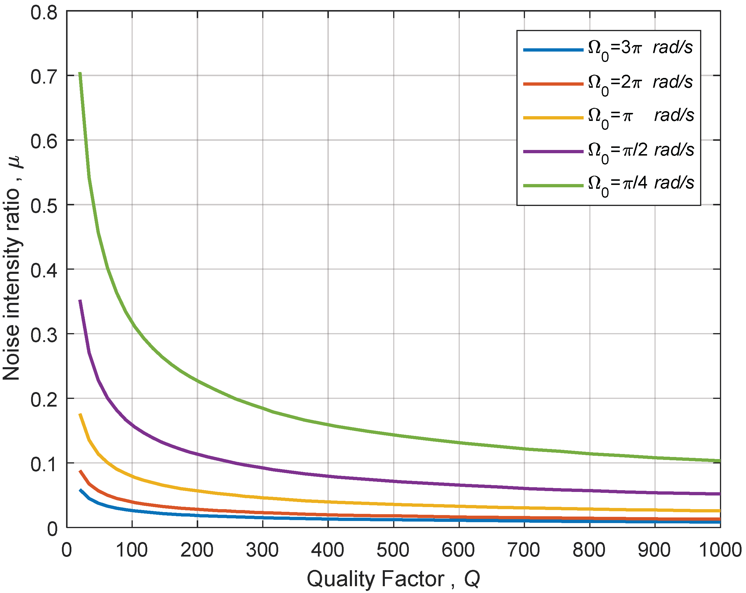
It is known that the gyroscopic systems are not immune to the external noise effects that can alter their dynamic behavior. Such noise usually stems from environmental and operational sources and can be exerted on the system at any frequency range depending on the source. Furthermore, the allowance of noise effects on the MEMS system is an important design factor, especially at low damping ratios (high quality factor) which is a characteristic feature of modern MEMS gyroscopic systems. Therefore, a parametric study is performed to assess the noise intensity stability threshold for a number of quality factor values at different input angular rates. To this end, an increment of the system quality factor of approximately 50 is employed and the system noise stability threshold is obtained via the bisection search method. Further refinement is employed in the low quality factor region for analyzing the predicted time response. Figure 7 shows that the noise intensity threshold is decreased at higher quality factors. Increasing the angular speed, for high quality factors, reduces the fluctuation noise intensity threshold value to a value less than 1% of the angular speed. In such cases, where the noise effects are of concern, use of an active disturbance rejection control has been shown to eliminate/reduce the noise effects (see, e.g., [19]). It may be noted that the present study is limited to the predictions of threshold values, while the actual applications, as well as the operating conditions may dictate the absolute levels of fluctuation required to cause system instability. It is worth noting that such predictions can only be achieved via laboratory or in situ measurements. The employed approach uses the assumption of noise in angular rate in the absence of angular acceleration. Owing to the non-differentiable nature of white noise, this term cannot be evaluated for the solution process followed for numerically solving the resulting SDE. This assumption limits the inclusion of the angular acceleration terms in the analysis; however, to overcome this difficulty, one can use the fluctuation in the angular acceleration, for low angular velocities, which is typical in the case of gyroscopes. Alternatively, a narrow band noise assumption for the angular velocity to simulate the velocity fluctuation is also feasible. These approaches are likely to increase the prediction accuracies, but are beyond the scope of the present study.
In addition, studies performed on varying input angular rates of practical significance for typical gyroscope applications revealed that the increase in angular velocity decreases noise thresholds. Further studies on the effect of the frequency mismatch, which originates form asymmetry in both of supporting springs stiffness and/or proof- mass are performed. A change of frequency mismatch for low and moderate values in the range up to 10% seems to have insignificant effects on the noise threshold. However, unrealistic frequency mismatch values close to 20% causes a reduction in the noise threshold. It is worth noting that such values for the frequency mismatch are not of practical significance under typical gyroscope operating conditions. It is expected that these results will lead to the identification of critical stability regions for this class of devices, which can then improve the device performance, reliability, and the design process.
5. Conclusions
The dynamic behavior of a mass-spring type MEMS-based single-axis vibratory gyroscope is investigated when subjected to stochastic fluctuations in the input angular rate. The effect of random fluctuations is introduced into the gyroscope governing equations to form stochastic differential equations that are discretized using the Milstien scheme to predict the response numerically. The Euler scheme, as well as the largest Lyapunov exponents, have also been used in this study as a validation tool due to the lack of analytical solutions and experimental data. A nonlinear decreasing trend of the obtained threshold values for the noise intensity at different quality factor values has been observed while a similar decreasing trend of noise thresholds with the angular rate increase is also predicted. Variations in the frequency mismatch have shown insignificant influence on system stability under typical gyroscope operating conditions. It is envisaged that the present quantitative predictions will lead to improvements in performance, reliability, and the design process for this class of devices via identification of critical stability regions.
Author Contributions
M.B. and S.F.A. formulated the system model; M.B. performed the numerical simulations; and M.B. and S.F.A. analyzed the results and wrote the manuscript.
Funding
This research was funded partially by Natural Science and Engineering Research Council (NSERC) of Canada discovery grant, grant# RGPIN/250432-2012 and scholarship awarded to the first author by Libyan-North American Scholarship program.
Acknowledgments
The support of the Natural Science and Engineering Research Council (NSERC) of Canada discovery grant and the Libyan-North American Scholarship program are acknowledged.
Conflicts of Interest
The authors declare no conflict of interest. The funding sponsors had no role in the design of the study; in the collection, analyses, or interpretation of data; in the writing of the manuscript; or in the decision to publish the results.
References
- Acar, C.; Schofield, A.; Trusov, A.; Costlow, L.; Shkel, A. Environmentally robust MEMS vibratory gyroscopes for automotive applications. IEEE Sens. J. 2009, 9, 1895–1906. [Google Scholar] [CrossRef]
- Xing, H.; Hou, B.; Lin, Z.; Guo, M. Modeling and compensation of random drift of MEMS gyroscopes based on least squares support vector machine optimized by chaotic particle swarm optimization. Sensors 2017, 17, 2335. [Google Scholar] [CrossRef] [PubMed]
- Younis, M.; Jordy, D.; Pitarresi, J. Computationally efficient approaches to characterize the dynamic response of microstructures under mechanical shock. J. Microelectromech. Syst. 2007, 16, 628–638. [Google Scholar] [CrossRef]
- Zuo, L.; Pei-Sheng, Z. Energy harvesting, ride comfort, and road handling of regenerative vehicle suspensions. J. Vib. Acoust. 2013, 135. [Google Scholar] [CrossRef]
- Schiehlen, W. White noise excitation of road vehicle structures. Sadhana 2006, 31, 487–503. [Google Scholar] [CrossRef] [Green Version]
- Passaro, V.M.N.; Cuccovillo, A.; Vaiani, L.; De Carlo, M.; Campanella, C.E. Gyroscope technology and applications: A review in the industrial perspective. Sensors 2017, 17. [Google Scholar] [CrossRef] [PubMed]
- Hosseini-Pishrobat, M.; Keighobadi, J. Robust vibration control and angular velocity estimation of a single-axis MEMS gyroscope using perturbation compensation. J. Intell. Robot. Syst. 2018, 90, 1–19. [Google Scholar] [CrossRef]
- Mochida, Y.; Tamura, M.; Ohwada, K. A micro machined vibrating rate gyroscope with independent beams for the drive and detection modes. Sens. Actuator A Phys. 2000, 80, 170–178. [Google Scholar] [CrossRef]
- Davis, W.O. Mechanical Analysis and Design of Vibratory Micro Machined Gyroscopes. Ph.D. Thesis, University of California, Berkeley, CA, USA, 2001. [Google Scholar]
- Asokanthan, S.F.; Wang, T. Dynamic instabilities in a single-axis gyroscope subjected to stochastic angular rate perturbations. Probab. Eng. Mech. 2009, 24, 600–607. [Google Scholar]
- Asokanthan, S.F.; Arghavan, S.; Bognash, M. Stability of ring-type MEMS gyroscopes subjected to stochastic angular speed fluctuation. ASME. J. Vib. Acoust. 2017, 139, 040904–040907. [Google Scholar] [CrossRef]
- Higham, D.J. An algorithmic introduction to numerical simulation of stochastic differential equations. SIAM Rev. 2001, 43, 525–546. [Google Scholar] [CrossRef]
- Schaffter, C.T. Numerical Integration of SDEs: A Short Tutorial; Swiss Federal Institute of Technology in Lausanne (EPFL): Lausanne, Switzerland, Unpublished work; 2010. [Google Scholar]
- Zotov, A.S.; Simon, B.R.; Prikhodko, I.P.; Trusov, A.A.; Shkel, A.M. Quality factor maximization through dynamic balancing of tuning fork resonator. IEEE Sens. J. 2014, 14, 2706–2714. [Google Scholar] [CrossRef]
- Kloeden, P.E.; Platen, E. Numerical Solution of Stochastic Differential Equations; Springer: Berlin, Germany, 1999. [Google Scholar]
- Higham, D.J.; Kloeden, P.E. MAPLE and MATLAB for Stochastic Differential Equations in Finance. Programming Languages and Systems in Computational Economics and Finance; Nielson, S.B., Ed.; Springer Science + Business Media: Dordrecht, The Netherlands, 2002. [Google Scholar]
- Yang, C.; Wu, Q. On stability analysis via Lyapunov exponents calculated from a time series using nonlinear mapping-a case study. Nonlinear Dyn. 2010, 59, 239–257. [Google Scholar] [CrossRef]
- Kliková, B.; Raidl, A. Reconstruction of phase space of dynamical systems using method of time delay. In WDS’11 Proceedings of the Contributed Papers: Part III—Physics; Matfyz Press: Prague, Czech Republic, 2011. [Google Scholar]
- Zheng, Q.; Dong, L.; Lee, D.H.; Gao, Z. Active disturbance rejection control for MEMS gyroscopes. IEEE Trans. Control Syst. Technol. 2009, 17, 1432–1438. [Google Scholar] [CrossRef]
Figure 1.
Single-axis mass-spring gyroscope.
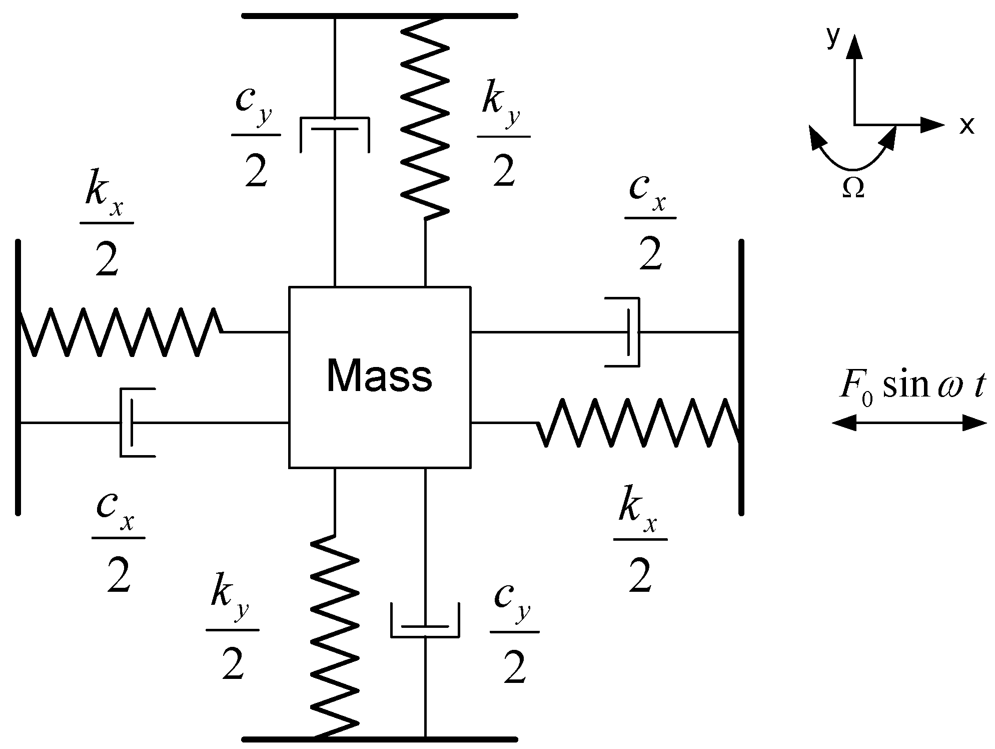
Figure 2.
Example of the stable time response.

Figure 3.
Example of the marginally stable time response.
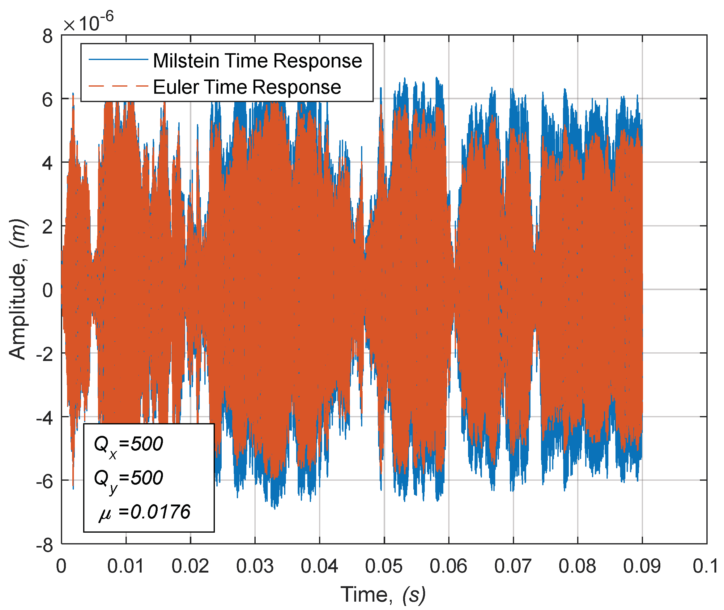
Figure 4.
Example of the unstable time response.

Figure 5.
Under-prediction of results by Euler scheme.
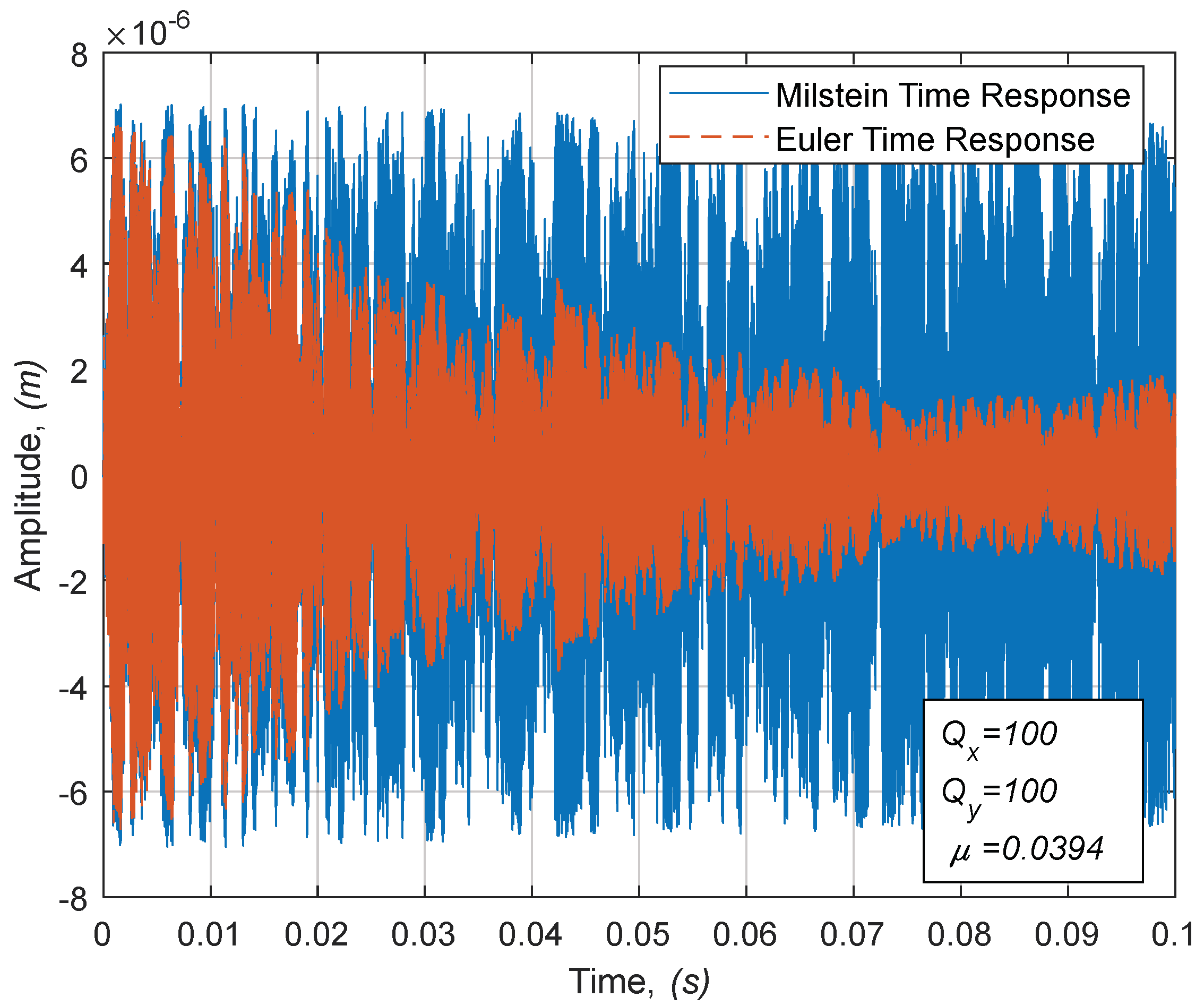
Figure 6.
Stability boundary in the space ().
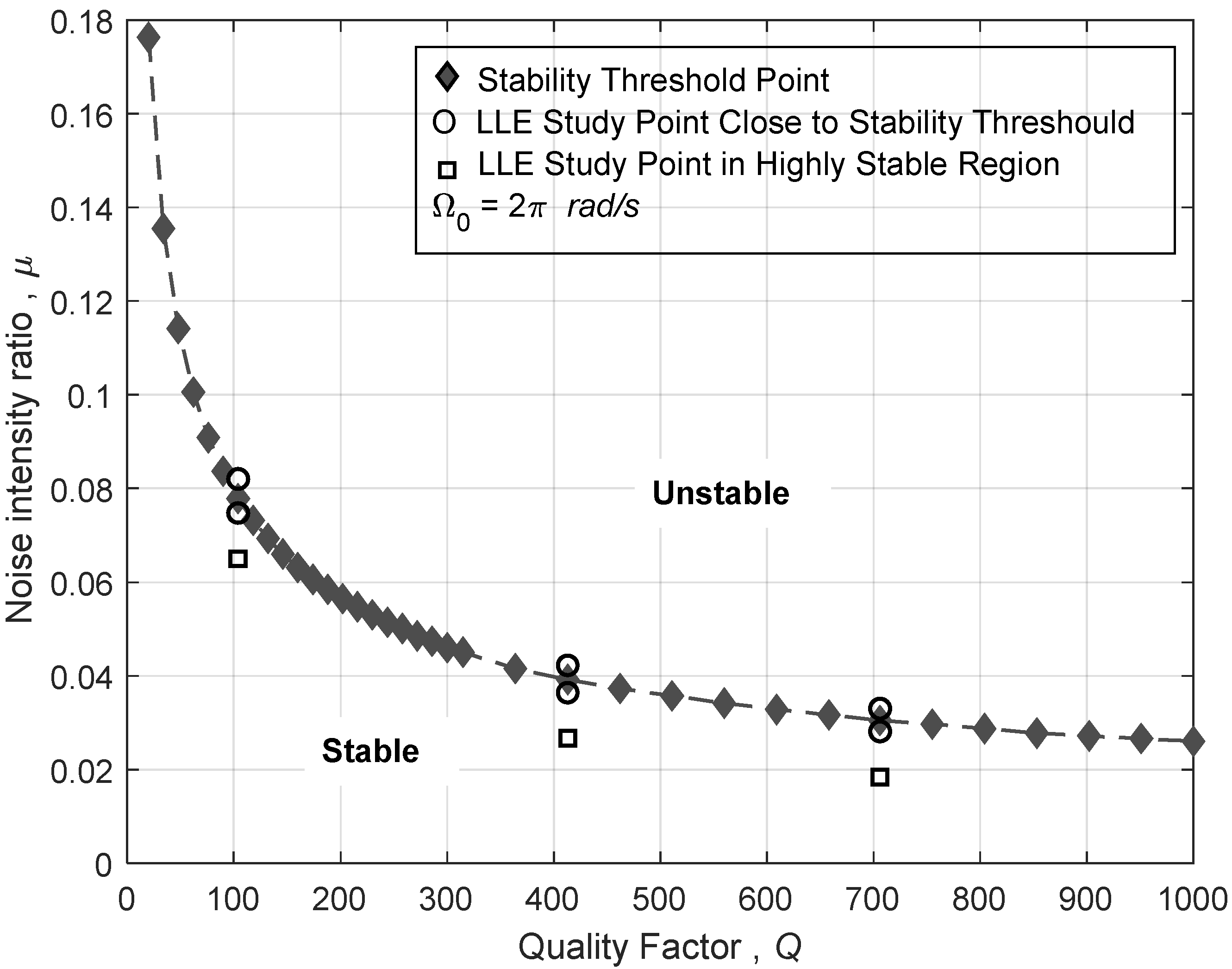
Figure 7.
Stability boundary in the space.

Table 1.
Single-axis gyroscope parameters [9].
Table 1.
Single-axis gyroscope parameters [9].
| Parameter | Notation | Value |
|---|---|---|
| Gyroscope mass | ||
| Nominal X-axis natural frequency | ||
| Nominal Y-axis natural frequency | ||
| X-axis quality factor | 20–1000 | |
| Y-axis quality factor | 20–1000 |
© 2018 by the authors. Licensee MDPI, Basel, Switzerland. This article is an open access article distributed under the terms and conditions of the Creative Commons Attribution (CC BY) license (http://creativecommons.org/licenses/by/4.0/).
Share and Cite
MDPI and ACS Style
Bognash, M.; Asokanthan, S.F. Stochastic Stability of a Class of MEMS-Based Vibratory Gyroscopes under Input Rate Fluctuations. Vibration 2018, 1, 69-80. https://doi.org/10.3390/vibration1010006
AMA Style
Bognash M, Asokanthan SF. Stochastic Stability of a Class of MEMS-Based Vibratory Gyroscopes under Input Rate Fluctuations. Vibration. 2018; 1(1):69-80. https://doi.org/10.3390/vibration1010006
Chicago/Turabian StyleBognash, Mohamed, and Samuel F. Asokanthan. 2018. "Stochastic Stability of a Class of MEMS-Based Vibratory Gyroscopes under Input Rate Fluctuations" Vibration 1, no. 1: 69-80. https://doi.org/10.3390/vibration1010006