Structure Damage Identification Based on Regularized ARMA Time Series Model under Environmental Excitation


1
State Key Laboratory of Coastal and Offshore Engineering, School of Civil Engineering, Dalian University of Technology, Dalian 116024, China
2
Department of Civil and Environmental Engineering, Shantou University, Shantou 515063, China
3
Smart Materials and Structures Laboratory, Department of Mechanical Engineering, University of Houston, Houston, TX 77004, USA
*
Author to whom correspondence should be addressed.
Vibration 2018, 1(1), 138-156; https://doi.org/10.3390/vibration1010011
Submission received: 6 August 2018
/
Revised: 28 August 2018
/
Accepted: 30 August 2018
/
Published: 3 September 2018
(This article belongs to the Special Issue Civil Engineering Applications of Structural Health Monitoring)
Abstract
:In this paper, a non-modal parametric method to identify structural damage using a regularized autoregressive moving average time series model under environmental excitation is proposed in combination with the virtual impulse response function. This method can use the structural vibration response to determine the damage caused to the structure during environmental excitation. Firstly, the virtual impulse response function is obtained by using the structural vibration response. Then, a regularized ARMA time series model is used to fit the virtual impulse response function. Based on the change of auto-regression coefficients in the regularization model under different damage cases, the structural damage is identified. The authors derive the regularization equation of an ARMA time series model to solve the problems in a time series model and obtain the regularization coefficient. Finally, this method is applied to a three-degrees-of-freedom chain structure and a three-floor shear structure of the Los Alamos National Laboratory (LANL). The experimental results show that the method based on the regularized ARMA time series model under environmental excitation can effectively identify the structural damage, which is a reliable method for damage identification. The regularized ARMA time series model can accurately extract signal features and has invaluable application prospects in the field of structural health monitoring.
1. Introduction
In recent years, along with the rapid development of sensor technology [1,2,3,4,5,6] and advanced algorithms [7,8,9], structural health monitoring [10] has gradually become an important part of the operation and management of basic civil facilities. Engineers perform damage detection [11,12,13,14,15] on the structure and repair it in time to avoid unnecessary loss of personal or public property. At present, the global damage detection based on the structural vibration characteristics [16] has become the core of the SHM field, including modal parametric methods and non-modal parametric methods [17]. The modal parametric methods are based on the fact that the modal parametric of the structure can reflect the structural damage, such as the natural frequency, mode shape [18], mode curvature, modal flexibility [19] and modal strain energy to identify the damage. However, the damage identification method based on a modal parametric cannot be applied successfully in practical engineering [20]. The main reason is that, although the accuracy of modal frequency measurement is high, it is not sensitive to structural damage, especially in the case of environmental changes. The actual measurement of mode shapes is inaccurate, and it is difficult to obtain high-order mode shapes. The non-modal parametric methods [21,22,23] use the structural vibration response data directly or extract information from the measured response data that can reflect structural damage through a certain transformation. Compared to the structural modal parametric methods, the non-modal parametric methods are convenient, accurate, and can meet the real-time requirements of structural health monitoring [24].
The damage identification method based on the regularized autoregressive moving average time series model under environmental excitation proposed in this paper is a kind of non-modal parametric method. This method combines the virtual impulse response function with the regularized ARMA time series for the first time, and uses the auto-regression coefficients of the regularized time series model to identify the structural damage. So-called environmental incentives generally include wind load excitation, earth pulsation excitation, and personnel vehicle load excitation. The experiments done in this paper are all based on the simulation of the earth’s pulsating environment. However, it can be seen from the theoretical deduction that this method is not limited to the environmental excitation of the earth pulsation.
The virtual impulse response function is a very effective non-modal parametric damage signal. It can not only effectively overcome the randomness of the environmental stimulus, but also reflects the inherent characteristics of the structure. Ding et al. [25] carried out wavelet packet transform on the virtual impulse response function and computed the wavelet packet energy spectrum of the virtual impulse response function. By applying this method to a benchmark model, the effective identification of structural damage and the robustness of environmental excitation were verified. Diao et al. [26] proposed the wavelet packet transform processing of the virtual impulse response function and computed the energy of the wavelet packet node. Using the wavelet packet node energy before and after damage as the damage feature vector, the location of structure damage was determined by combining the pattern classification function of BP neural network, and the results show the effectiveness of the method and the robustness of environmental excitation.
The damage detection method based on time series analysis is also an effective non-modal parametric method. Time series analysis was a method originally used to analyze time series data in order to define the statistical characteristics of data and predict its future trends. Its application was initially in the economic and electrical engineering field. In recent years, time series models have been increasingly valued by SHM researchers. Sohn et al. [27] combined an autoregressive model with an externally derived autoregressive model (ARX) to propose a damage detection method, and the residual error was used as a damage feature to identify structural damage. Mei et al. [23] used an autoregressive model with external inputs (ARX model) to quantify changes in mass, stiffness, and damping in numerical models using acceleration, velocity, and displacement data. Liu et al. [28] used monitoring data to establish an ARMA model and used the principal component analysis method to extract new structural damage characteristics from the model’s autoregressive coefficients. A t-test was used to examine whether there was a significant change in the index before and after damage. Then it was applied to the finite element model of a three-span continuous beam with one section. The experimental results show that this method can effectively extract the damage information from the monitoring data.
Although there are many investigations in the damage detection of the time series model, there is a big problem with the analysis of the time series model. That is, under certain conditions, the system of equations will produce ill-conditioned problems, causing the time series model to be ill-posed. This will make the model coefficient very unstable [29]. In response to this problem, many scholars have proposed a regularization method for the time series model; however, they only derived the regularization equation of the AR model [30]. Based on the regularization of the AR model, the authors further derive the regularization method of the ARMA model. The selection of a regularization coefficient is described in detail. The authors have found that the regularized time series model can not only simulate and predict the time series, but also accurately extract the characteristics of the signal, and it has good application prospects in the field of damage identification.
2. Virtual Impulse Response Function
The excitation and response have the following relationship in the frequency domain:
where is the Fourier transform for response, is the Fourier transform of the excitation, and is a frequency response function.
The cross-spectrum density of reference point response (virtual excitation) and measuring point response is . The auto-spectral density of reference point is , as shown in the following formula:
where and are the Fourier transform of measuring point response and reference point response . is the complex conjugate of .
It is known from Equation (1) that and can be expressed as follows:
Equation (3) can be substituted into Equation (2) and the frequency response function is computed by the following formula:
It can be seen from the above derivation that the frequency response function of a two-point response can effectively eliminate the influence of excitation. In other words, the virtual impulse response function obtained by inverse Fourier transform to the spectrum response function can effectively restrain the randomness and uncertainty of the environment excitation, and thus has strong robustness to environmental excitation [31].
3. Regularized ARMA Time Series Model
3.1. Introduction of ARMA Time Series Model
The ARMA time series model can be expressed as in Equation (5), where is an autoregressive coefficient, is a moving average coefficient, represents the value of the time series at time t and represents the disturbance entering the system at time t:
If , the model becomes a centralized ARMA model:
Adding the genetic operators, the centralized time sequence model can be abbreviated as . It is obvious that the problem is two-fold. The first and probably the most important task is the successful determination of the predictor’s order p and q. The second task is the estimation of the predictor’s matrix coefficients and . Determining the order of the ARMA process is usually the most important part of the problem. Over the past years, substantial literature has been produced on this problem and various different criteria, such as Akaike’s, Rissanen’s, Schwarz’s, and Wax’s [32,33,34,35,36], have been proposed to implement the order selection process. The ARMA model order identification and parametric estimation were accomplished by minimizing the Akaike’s Corrected Information Criterion (AIC):
where n is the sample size and p, q is the model order and is a maximum likelihood estimate of R under the assumption that ARMA is the correct model order [37].
3.2. Regularization of ARMA Time Series
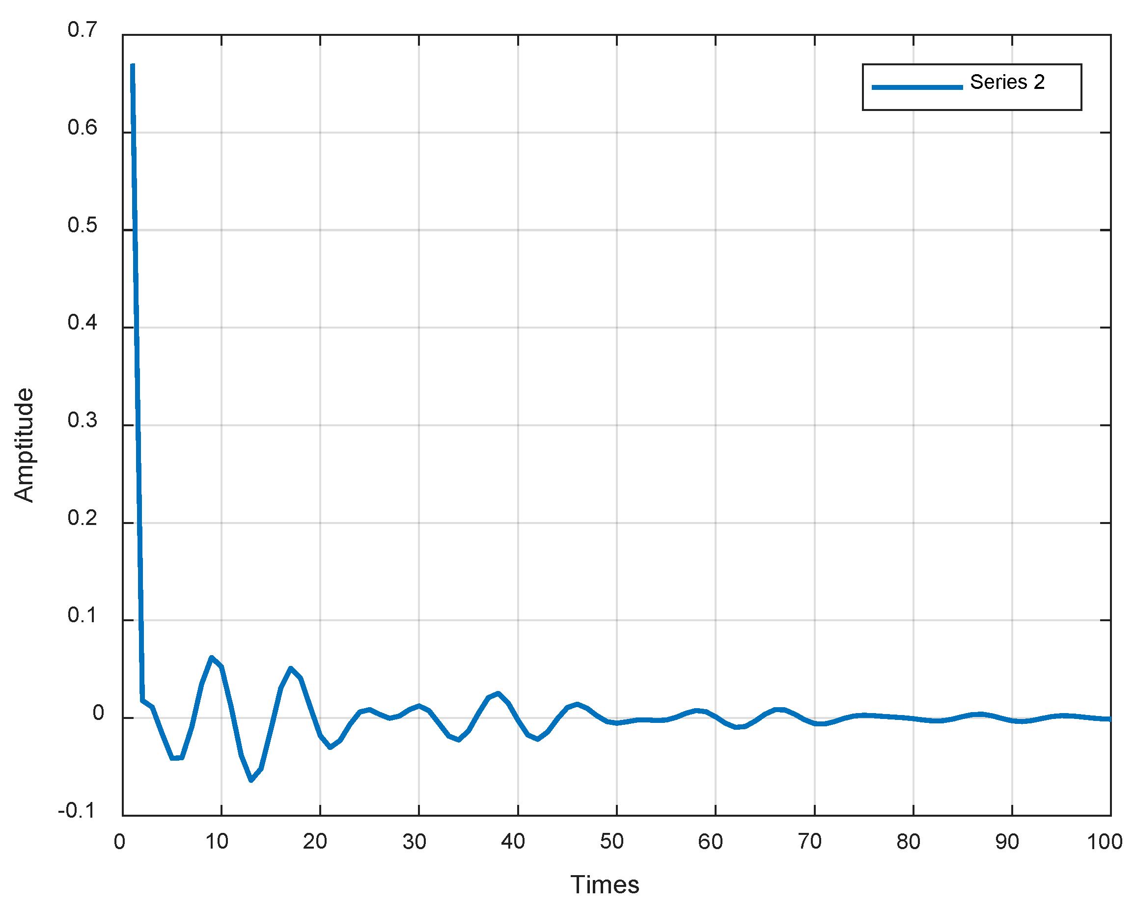
The time series model has strong feature extraction capabilities. However, in the practical application process, it shows some uncertainty. This uncertainty can be illustrated by the following example: there are two slightly different signals, as shown in Figure 1 and Figure 2, where the abscissa is the time and the ordinate is the amplitude of the signal.
Obviously, the difference between them cannot be identified with the naked eye. We used the same time series model to fit them and extracted their AR coefficients as shown in Figure 3. The abscissa indicates the sequence of AR coefficients, and the ordinate indicates the value of the AR coefficients.
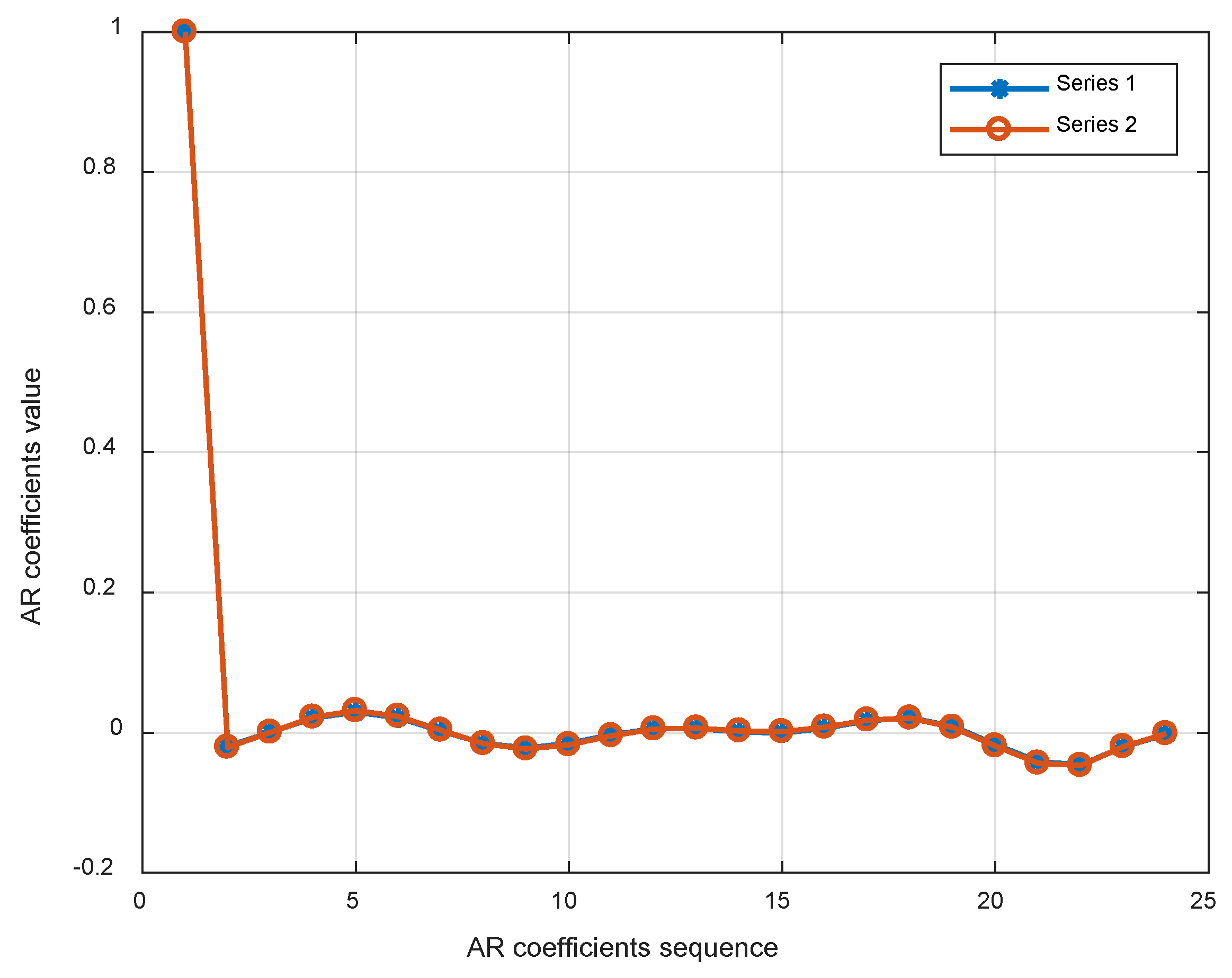
From Figure 1, Figure 2 and Figure 3, it can be seen that although the signal has only a few differences, the AR coefficients are extremely unstable. This shows that the AR coefficients of the non-regularized ARMA model cannot reflect the characteristics of the signal. As mentioned earlier, under certain conditions, the system of equations will produce problems; however, using regularization methods, such problems can be eliminated. If a regularized ARMA model is used and the regularization coefficient is chosen to be 0.1, then the AR coefficient of the two signals is calculated as shown in Figure 4. As can be seen from Figure 4, the regularized AR coefficients tend to be stable and can accurately reflect the characteristics of the signal. Regularization is a technique for specifying the constraints on the flexibility of a model, thereby reducing uncertainty in the estimated parametric values.
Ideally, the parametric of a good model should minimize the mean square error (MSE), given by a sum of systematic error (bias) and random error (variance):
The minimization is thus a tradeoff in constraining the model. A flexible (high-order) model gives small bias and large variance, whereas a simpler (low-order) model results in larger bias and smaller variance errors. Regularization allows for better control over the bias versus variance tradeoff by introducing an additional term in the minimization criterion that penalizes the model flexibility.
3.3. Derivation of Regularized ARMA Time Series
In order to explain how the regularization method eliminates the ill-posed problems of ill-conditioned equations, the authors derive the regularization formula of the ARMA time series model using the least-squares method. This also paves the way for the selection of regularization coefficients.
Equation (6) can be transformed into the least-squares format. First, formulate the equation as follows:
After making the above decomposition, we can obtain the least-squares format of the ARMA model, as follows:
If there are N sample data, and , we can combine the data into Equation (10), which can be expressed as follows:
In Equation (11):
Then the least square estimate of coefficient b is:
If the elements of the matrix are accumulatively summed up by data with very close values and the columns in have a complex collinearity, the numerical solution of the ill-conditioned equation group b will be unstable. Therefore, when using the general ARMA time series model to fit the same signal, the obtained AR coefficient is unstable.
The inversion operation in Equation (12) is the cause of the ill-posed problems of the ARMA model. The regularization method is usually used to eliminate the ill-posed phenomenon of the matrix. This study eliminates the ill-posed problems of the ARMA model by adding a regularization factor to the matrix.
Add a regularization factor to so that it becomes , then Equation (12) will become the following equation:
Equation (13) is the regularized time series ARMA model. The model can improve the ill-posed problems of the matrix. Obviously, when the regularization factor , the above two equations are equal.
3.4. The Selection of Regularization Coefficient α
Solving Equation (13) is the focus of this study, and Equation (13) is also called ridge regression [38]. The trajectory of b with the change of is known as the ridge trace. The difficulty of applying the regularization lies in how to efficiently find the optimal regularization coefficient. A number of choices are available in the literature, including the L-curved method, the S-curve method and the generalized cross-validation (GCV) method [39]. These methods operate on the basis of the singular value decomposition of the coefficient matrix and are computationally effective when the matrix has a small size. However, when the matrix size increases, the computational efficiency decreases dramatically. In the actual calculation, we fit the two almost identical signals and extract the AR coefficients using a regularized time series model. When the regularization coefficient is small, the differences in the AR coefficients are large. As the regularization coefficient gradually increases, the AR coefficients of the two similar signals gradually become the same. Therefore, when the regularization coefficient is gradually increased, the norm of the AR coefficient is taken as an index for judging the stability of the AR coefficient. A curve in which a norm of the AR coefficient changes with the regularization coefficient is plotted, and the value of the regularization coefficient is determined when the image tends to be stable. In addition, as can be seen from Equation (13), with the increase of , the absolute values of each element in b tend to become smaller, and the deviation from the correct value of the coefficient becomes larger. When approaches infinity, the values of the b-matrix approach zero. Therefore, we should choose a value of that is as small as possible. This is because the smaller the value of is, the smaller the deviation between the regularized model and the actual data, which makes the model data more responsive to the characteristics of the original data [40]. The selection of the regularization coefficient will be described in detail in the damage identification process below.
3.5. Regularized ARMA Time Series Modeling
The data that we usually process are a non-stationary time series with linear trends or periodic changes. In this regard, we should perform data processing first, that is, data smoothing. Generally, data are processed by first-order or two-order difference treatment. If a sequence can be determined as a smooth non-white noise sequence by sequence preprocessing, the sequence can be modeled directly using an ARMA model [41]. The modeling process is as follows:
- Determine the sample Auto Correlation Function (ACF) and Partial Auto Correlation Function (PACF) of the signal to be simulated.
- Choose the appropriate model based on the sample autocorrelation coefficient and partial autocorrelation coefficient properties.
- Determine the model order using AIC or other criteria.
- Validate the model. If the geometric model does not pass the test, go to Step 2, reselect the model, and fit again.
- Optimize the model. If the fitted model passes the test, then it still moves to Step 3, taking full consideration of the possibilities, creating a number of quasi-models, and selecting the optimal model from all the tested fitted models.
- Calculate regularization coefficients and regularization time series models based on optimal model parametric.
- Extract the AR coefficients as feature vectors from the regularized time-series fitting optimal model.
4. Damage Identification Procedure
The virtual impulse response function can effectively restrain the randomness and uncertainty of the environmental excitation, and characterize the intrinsic characteristics of structural dynamical systems under environmental excitation. What is more noteworthy is that the virtual impulse response function obtained from the reference point for virtual excitation and other measurement points is a stationary non-white noise sequence. Therefore, it is possible to use the ARMA model to fit and extract signal damage features. Specific steps are as follows:
- For a structured health monitoring system in which the sensors have been placed, the virtual impulse response function is obtained by comparing a large vibration response with another response where the damage may occur.
- Use the regularized ARMA time series model to fit the obtained virtual impulse response and extract the AR coefficient of the best-fit model as the damage feature vector.
- Compare the AR coefficient extracted from the undamaged working condition and damage condition and calculate the damage index.
The damage index (DI), as a 1 norm of AR coefficient for damage case and healthy case, can be calculated by
where n is the number of repeated trials of different samples, and i is the different damage cases.
5. Numerical Simulation
5.1. Three-Degrees-of-Freedom Chain Structure
To illustrate the effectiveness of the method, a three-degrees-of-freedom chain structure is numerically simulated. The structure is shown in Figure 5. The mass matrix and stiffness matrix of the structure are shown in Equation (15). A random Gaussian noise is applied to the bottom of the three-degrees-of-freedom chain structure to simulate environmental excitations.
After knowing the stiffness and mass matrix of the structure, it is easy to find its natural frequency: . The corresponding damping ratio of each mode is 0.05. The initial speed and displacement are set to 0. The inertia force vector , the sampling frequency is 100 Hz, and the vibration response of each particle of the structure is recorded for 50 s. The structure was stimulated with random Gaussian noise under different operating conditions, and each operating case was independently operated 10 times.
The damage to the structure is shown in Table 1, which gives the gradual reduction of the stiffness . The reason why stiffness decreases is that the reduction in the top stiffness has the least influence on the damage of the overall structure and the resulting damage is the most difficult to identify.
5.2. Damage Identification Process
The virtual impulse response function is obtained by using the response at the point and the response at the point . The response at point is used as a virtual stimulus, and the response of point is taken as the reference point. Based on the previously described time series modeling method, the ARMA time series is modeled for the first 100 data points of the virtual impulse response.
Taking Case 1 as an example, the ACF and PACF of the virtual impulse response are shown in Figure 6. From the figure, the abscissa is lag and the ordinate is the value of ACF and PACF respectively, we can see that the autocorrelation coefficients show tailing and the partial autocorrelation coefficients show truncations. In theory, the AR model should be used for simulation. However, we choose the ARMA model here since the regularized ARMA model can also reflect the nature of the AR model. In this way, the method can be unified without having to tangle with the choice of the model.
Since only 100 data points are selected, the ARMA model order has a maximum value of 25. Based on the AIC criterion, we calculate the AIC coefficients of different combinations of model orders p and q. When the AIC coefficient is the lowest, the orders p and q are 25 and 21, respectively. The model coefficients are repeatedly optimized according to the modeling method of the time series model. When the model fits optimally, the orders p and q are 25 and 24, respectively. This model will be used to fit the virtual impulse response of all working cases. Then, we need to find the regularization coefficient.
As mentioned earlier, only the regularized ARMA time series can be used to correctly reflect the characteristics of the signal. Taking Case 1 as an example, the regularization coefficient was selected from 0.00002 to 0.001, gradually rising by 0.00002. When the regularization coefficient is small, the AR coefficients of two identical signals are very different, which is shown in Figure 3. As the regularization coefficient increases, their AR coefficients will tend to be equal, as shown in Figure 4. In order to decide whether the AR coefficient is stable, the 1 norm of the AR coefficients of the two very similar signals under the same regularization coefficient is used as an indicator of the stability of the discriminant coefficient. The result of the calculation is shown in Figure 7. The ordinate is the 1 norm of the AR coefficients of the two very similar signals under the same regularization coefficient; the abscissa is 50 sets of data corresponding to different regularization coefficients.
From Figure 7, it can be seen that the AR coefficient tends to be stable at the 40th data. Therefore, the regularization coefficient should be greater than 0.008 , so the regularization coefficient is chosen to be 0.05. After determining the order and regularization coefficients of the ARMA time series model, we use the same regularization model to fit the virtual impulse response under different working cases and calculate the damage index. When the ARMA time series model fits above 90% in all working cases, good results can be obtained.
Taking Case 1 (no damage), Case 4 (15% damage), and Case 7 (30% damage) as examples, the distribution of regularized AR coefficient values after 10 independent operations is plotted in Figure 8. It can be clearly seen from Figure 8 that the AR coefficient of each operation is almost unchanged under the same working case, while the AR coefficients under different working cases are different. As the damage gradually increases, the difference in AR coefficients gradually increases, so the corresponding damage index also gradually increases. The degree of simulation has reached 93% at this time.
Figure 9a shows the results of the damage indicators of the three-degrees-of-freedom chain structure after 10 independent operations under different operating cases. Each 10 sets of data on the abscissa indicate one damage case. There are a total of 70 sets of data on the abscissa because there are seven different sets of damage conditions. From Figure 9a we can see that as the damage increases, the damage index gradually increases. This result demonstrates the effectiveness of this method. It can be found that the damage index effectively identifies the occurrence of damage when the structure is damaged slightly (5–10%).
Figure 9b illustrates the damage identification from another perspective. The abscissa indicates the damage cases, and the ordinate indicates the damage index DI. As can be seen from Figure 9b, the damage index is stable under each operating condition. Under different working cases, the damage index DI increases with the increase of damage. The reliability of the damage index is also verified.
6. Verification Using the Data of the Alamos Three-Floor Shear Structure
6.1. Test Structure Description
The three-story frame structure shown in Figure 10 is used as a damage detection test bed. The structure consists of aluminum columns and plates assembled using bolted joints. The structure slides on rails that allow movement in the x-direction only. At each floor, four aluminum columns are connected to the top and bottom aluminum plates forming a (essentially) four-degree-of-freedom system. Additionally, a center column is suspended from the top floor. This column is used as a source of damage that induces nonlinear behavior when it comes into contact with a bumper mounted on the next floor. The position of the bumper can be adjusted to vary the extent of impact that occurs at a particular excitation level. A schematic representation of the structure is shown in Figure 11.
An electrodynamic shaker provides a lateral excitation to the base floor along the centerline of the structure. We used the vibration of the bottom electric shaker to simulate the environmental excitation of the earth’s pulsation. The structure and shaker are mounted together on an aluminum baseplate and the entire system rests on rigid foam. The foam is intended to minimize extraneous sources of unmeasured excitation from being introduced through the base of the system. A load cell (Channel 1) with a nominal sensitivity of 2.2 mV/N was attached at the end of a stinger to measure the input force from the shaker to the structure. Four accelerometers (Channels 2–5) with nominal sensitivities of 1000 mV/g were attached at the centerline of each floor on the opposite side from the excitation source to measure the system response. Because the accelerometers are mounted at the centerline of each floor, they are insensitive to torsional modes of the structure.
The analog sensor signals were discretized into 8192 data points sampled at 3.125 ms intervals, corresponding to a sampling frequency of 320 Hz. These sampling parametric yield time series were 25.6 s in duration. A band-limited random excitation in the range of 20–150 Hz was used to excite the structure. This excitation signal was chosen in order to avoid the rigid body modes of the structure that are present below 20 Hz. Structural damage occurs in the form of stiffness reduction. The stiffness changes were introduced by reducing the stiffness of one or more of the columns by 87.5%. This process was executed by replacing the corresponded column with one that had half the cross-sectional thickness in the direction of shaking. Alamos three-floor shear structure damage is divided into five kinds of working states, as shown in Table 2. For example, 1BD in State #2 refers to the column of the structure where the planes B and D intersect at the first layer in Figure 11. In State #3, the stiffness of both columns is reduced by 87.5%. As above, States #4 and #5 represent the damage state of the second layer.
6.2. Damage Identification Process
In the original data for the Alamos three-layer shear structure, there are 50 different sets of data, which were collected by sensors under different environmental excitations. The environmental excitation refers to the earth pulsation excitation, which is simulated by applying an exciter at the bottom of the structure. In this paper, 10 different sets of data are used to identify the Alamos three-layer shear structure under different damage states.
First of all, there is still a need to find the virtual impulse response function, in which the selection of the reference point is particularly important. Generally, a sensor position with a larger vibration amplitude is used as a virtual pulse reference point. In this example, the sensor response of the top-level Channel 5 is selected as the reference point. Under different damage conditions, the virtual impulse response function between Channel 5 and Channel 3 is calculated. The first 100 data points of virtual pulses are selected, and then a regularized time series model is used to fit the virtual impulse response function. Before using the time series model, it is necessary to obtain the ACF and PACF of the virtual impulse response function. Taking State #1 as an example, the ACF and PACF of the virtual impulse response function are shown in Figure 12.
Then we used AIC criteria to determine the orders of the model. When the AIC coefficient is the smallest, the orders p and q are 25 and 24, respectively. Next, the regularization coefficient is determined through the method proposed above. After adding the regularization coefficient, the regularized ARMA (25, 24) model is used to fit two similar virtual pulse response signals under the same damage states. The regularization coefficient increases gradually from 0.002 to 0.1, with each increase set to 0.002, for a total of 50 groups of data. With the increase in the regularization coefficient, two AR fitting coefficients tend to be stable. Under the same regularization coefficient, the 1 norm of the AR coefficients obtained by two simulations is taken as an indicator of the stability of the discriminant coefficient. The result is shown in Figure 13, where the ordinate is the 1 norm of the AR coefficients of two very similar signals under the same regularization coefficient, and the abscissa is 50 sets of data corresponding to different regularization coefficients.
As can be seen from Figure 13, the AR coefficients of the two sets of similar signals tend to stabilize after the 50th set of data. Therefore, the regularization coefficient should be greater than 0.1 (0.002 50). The regularization coefficient is chosen to be 1 here. In the existing 50 groups of data, 10 groups of data are randomly selected to identify the damage of five working states using the above method.
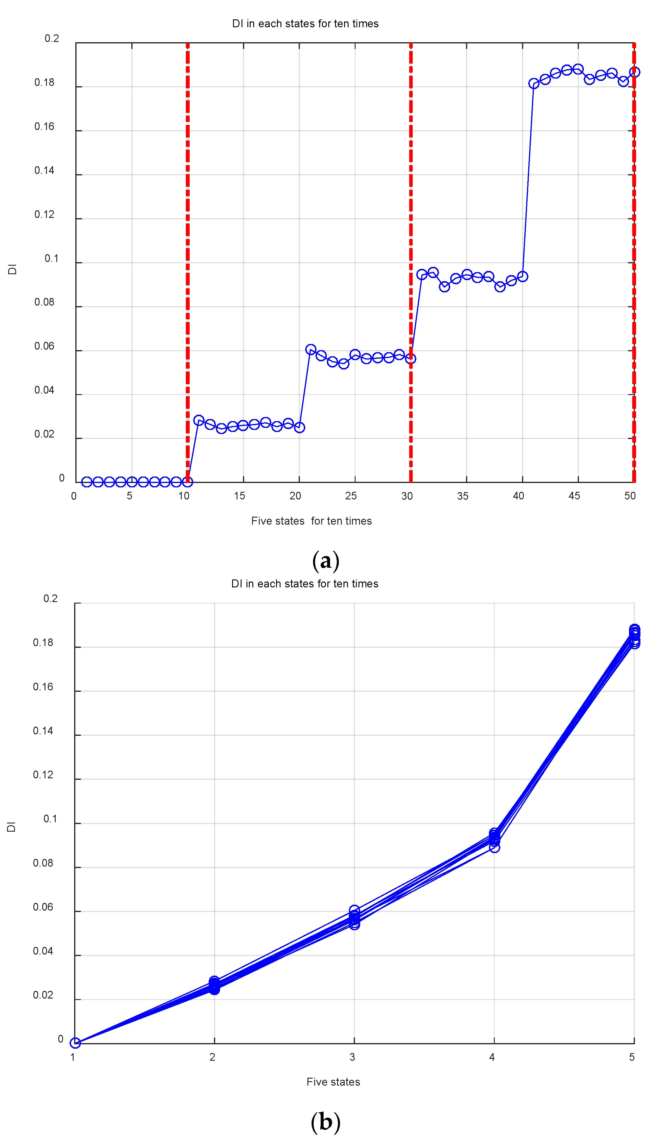
The damage identification results are shown in Figure 14a. The five intervals of abscissa represent five different working states. In each state, 10 groups of data are expanded in sequence, and the ordinate is the damage index DI. It can be clearly seen from the figure that the damage index of each working state tends to be stable, and the damage index also becomes larger when the degree of damage becomes larger. The red dashed line in the figure is to separate the state of each layers. As the damage of the first and second layers occurs alone, it is hard to compare the extent of the overall damage. However, it can be concluded from the damage index that the damage of the first and second floors are gradually increasing. Figure 14b is another representation of the result. The abscissa indicates the damage states and the ordinate represents the damage index. The same results can be seen.
7. Discussion
In order to make the method closer to reality, it is applied to the laboratory structure of Alamos. The current limitation of this study is that the location of the damage needs to be found. Moreover, we did not apply this method to a real structure. We will extend this method in future research and apply it to an actual structure. As for the determination of the damage degree, it can be seen from the damage identification result that the damage index will become larger as the damage degree increases, which is a gradual change. In practice, we can give a threshold. When the damage index is greater than this threshold, the structure will cease to be used.
8. Conclusions
In this paper, the regularization equation of the ARMA time series model is derived and the structural damage is identified by combining a regularized time series model with a virtual impulse response function. The results of numerical experiments and a test of the Alamos three-layer shear structure show that the method is effective for nonparametric damage identification. The regularized time series model can accurately extract the characteristics of the signal. The advantages of the proposed damage identification method can be summarized as follows:
- It has strong robustness to environmental excitation and can effectively identify damage based on environmental excitation.
- The direct use of structural vibration response for non-parametric damage identification has strong practicality and allows for real-time damage monitoring.
- The results of numerical simulations show that the method is sensitive to slight damage to the structure. Even a 5% reduction in stiffness can be identified.
The method proposed in this paper makes full use of the characteristics of the virtual impulse response function and the regularized time series model. The experimental results reflect the signal feature extraction ability of the regularized time series model. It can be seen that the regularized time series model has inestimable application prospects in the field of structural health monitoring.
Author Contributions
X.Z. and D.L. conceived this method and operated the software to implement it. G.S. and D.L. manage the data and verify the results. X.Z. wrote the paper and all authors read and approved the final manuscript.
Funding
This research was funded by the support of the National Natural Science Foundation of China (Nos. 51121005, 51578107 and 51778103), the National 973 Project of China (No. 2015CB057704), and Research Fund (DUT18LAB07 and NTF18012).
Conflicts of Interest
The authors declare no conflict of interest.
References
- Li, D.S.; Zhang, Y.; Ren, L. Sensor deployment for structural health monitoring and their evaluation. Adv. Mech. 2011, 41, 39–50. [Google Scholar]
- Wang, J.; Qin, L.; Song, W.; Shi, Z.; Song, G. Electromechanical Characteristics of Radially Layered Piezoceramic/Epoxy Cylindrical Composite Transducers: Theoretical Solution, Numerical Simulation and Experimental Verification. IEEE Trans. Ultrason. Ferroelectr. Freq. Control 2018. [Google Scholar] [CrossRef] [PubMed]
- Kong, Q.; Fan, S.; Bai, X.; Mo, Y.L.; Song, G. A novel embeddable spherical smart aggregate for structural health monitoring: Part I. Fabrication and electrical characterization. Smart Mater. Struct. 2017, 26, 095050. [Google Scholar] [CrossRef]
- Kong, Q.; Fan, S.; Mo, Y.L.; Song, G. A novel embeddable spherical smart aggregate for structural health monitoring: Part II. Numerical and experimental verifications. Smart Mater. Struct. 2017, 26, 095051. [Google Scholar] [CrossRef]
- Yin, H.; Wang, T.; Yang, D.; Liu, S.; Shao, J.; Li, Y. A smart washer for bolt looseness monitoring based on piezoelectric active sensing method. Appl. Sci. 2016, 6, 320. [Google Scholar] [CrossRef]
- Feng, D.M.; Feng, M.Q. Computer vision for SHM of civil infrastructure: From dynamic response measurement to damage detection—A review. Eng. Struct. 2018, 156, 105–117. [Google Scholar] [CrossRef]
- Xu, Y.; Luo, M.; Li, T.; Song, G. ECG Signal de-noising and baseline wander correction based on CEEMDAN and wavelet threshold. Sensors 2017, 17, 2754. [Google Scholar] [CrossRef] [PubMed]
- Shao, J.; Wang, T.; Yin, H.; Yang, D.; Li, Y. Bolt looseness detection based on piezoelectric impedance frequency shift. Appl. Sci. 2016, 6, 298. [Google Scholar] [CrossRef]
- Xu, B.; Zhang, T.; Song, G.; Gu, H. Active interface debonding detection of a concrete-filled steel tube with piezoelectric technologies using wavelet packet analysis. Mech. Syst. Signal Process. 2013, 36, 7–17. [Google Scholar] [CrossRef]
- Kong, Q.; Zhu, J.; Ho, M.; Song, G. Tapping and Listening: A New Approach to Bolt Looseness Monitoring. Smart Mater. Struct. 2018. [Google Scholar] [CrossRef]
- Lu, G.; Feng, Q.; Li, Y.; Wang, H.; Song, G. Characterization of ultrasound energy diffusion due to small-size damage on an aluminum plate using piezoceramic transducers. Sensors 2017, 17, 2796. [Google Scholar] [CrossRef] [PubMed]
- Kong, Q.; Robert, R.H.; Silva, P.; Mo, Y.L. Cyclic crack monitoring of a reinforced concrete column under simulated pseudo-dynamic loading using piezoceramic-based smart aggregates. Appl. Sci. 2016, 6, 341. [Google Scholar] [CrossRef]
- Du, G.; Kong, Q.; Zhou, H.; Gu, H. Multiple cracks detection in pipeline using damage index matrix based on piezoceramic transducer-enabled stress wave propagation. Sensors 2017, 17, 1812. [Google Scholar] [CrossRef] [PubMed]
- Xu, B.; Song, G.; Masri, S.F. Damage detection for a frame structure model using vibration displacement measurement. Struct. Health Monit. 2012, 11, 281–292. [Google Scholar] [CrossRef]
- Li, H.N.; Li, D.S. Safety assessment, health monitoring and damage diagnosis for structures in civil engineering. Earthq. Eng. Eng. Vib. 2002, 22, 82–90. [Google Scholar]
- Fan, W.; Qiao, P.Z. Vibration based Damage Identification Methods: A Review and Comparative Study. Struct. Health Monit. 2010, 9, 83–111. [Google Scholar]
- Alamdari, M.M.; Samali, B.; Li, J. Damage localization based on symbolic time series analysis. Struct. Control Health Monit. 2015, 22, 374–393. [Google Scholar] [CrossRef]
- Siebel, T.; Friedmann, A.; Koch, M.; Mayer, D. Assessment of Mode Shape-Based Damage Detection Methods under Real Operational Conditions. In Proceedings of the 6th European Workshop on Structural Health Monitoring, Dresden, Germany, 3–6 July 2012. [Google Scholar]
- Tomaszewska, A. Influence of statistical errors on damage detection based on structural flexibility and mode shape curvature. Comput. Struct. 2010, 88, 154–164. [Google Scholar] [CrossRef]
- Wu, S.; Wei, Z.; Wang, S.; Wang, B.; Li, Y. Damage Identification Based on AR Model and PCA. J. Vib. Meas. Diagn. 2012, 32, 841–845. [Google Scholar]
- Gul, M.; Catbas, F.N. Statistical pattern recognition for Structural Health Monitoring using time series modeling: Theory and experimental verifications. Mech. Syst. Signal Process. 2009, 23, 2192–2204. [Google Scholar] [CrossRef]
- Lakshmi, K.; Rama Mohan Rao, A. A robust damage-detection technique with environmental variability combining time-series models with principal components. Nondestruct. Test. Eval. 2014, 29, 357–376. [Google Scholar] [CrossRef]
- Mei, Q.; Gul, M. An Improved Methodology for Anomaly Detection Based on Time Series Modeling; Springer: New York, NY, USA, 2013; pp. 277–281. [Google Scholar]
- Tributsch, A.; Adam, C. An enhanced energy vibration-based approach for damage detection and localization. Struct. Control Health Monit. 2018. [Google Scholar] [CrossRef]
- Ding, Y.L.; Li, A.Q.; Miao, C.Q. Structural damage alarming method based on wavelet packet analysis by ambient vibration test. Chin. J. Appl. Mech. 2008, 25, 366–370. [Google Scholar]
- Diao, Y.S.; Zhang, Q.L.; Meng, D.M. Damage Localization of Offshore Platform Based on the Virtual Impulse Response Function. Adv. Mater. Res. 2012, 368–373, 1676–1680. [Google Scholar] [CrossRef]
- Sohn, H.; Farrar, C.R.; Hunter, N.F.; Worden, K. Structural Health Monitoring Using Statistical Pattern Recognition Techniques. J. Dyn. Syst. Meas. Control 2001, 123, 706–711. [Google Scholar] [CrossRef] [Green Version]
- Liu, Y.; Li, A.Q.; Ding, Y.L.; Fei, Q.G. Time Series Analysis with Structural Damage Feature Extraction and Alarming Method. Chin. J. Appl. Mech. 2008, 25, 253–257. [Google Scholar]
- Aswolinskiy, W.; Reinhart, F.; Steil, J. Impact of Regularization on the Model Space for Time Series Classification. In Proceedings of the New Challenges in Neural Computation, Bruges, Belgium, 27–29 April 2015; pp. 49–56. [Google Scholar]
- LI, T.; Tang, L.M.; Shi, S.Y. Regularized time series AR model and its application. J. Transp. Sci. Eng. 2009, 25, 24–28. [Google Scholar]
- Li, A.Q.; Miu, C.Q. Health Monitoring of Bridge Structures; China Communications Press: Beijing, China, 2009. [Google Scholar]
- Akaike, H. Fitting autoregressive models for prediction. Ann. Inst. Stat. Math. 1969, 21, 243–247. [Google Scholar] [CrossRef]
- Rissanen, J. Modeling by shortest data description. Automatica 1978, 14, 465–471. [Google Scholar] [CrossRef]
- Rissanen, J. A predictive least squares principle. J. Math. Control Inf. 1986, 3, 211–222. [Google Scholar] [CrossRef]
- Schwarz, G. Estimation of the dimension of the model. Ann. Stat. 1978, 6, 461–464. [Google Scholar] [CrossRef]
- Wax, M. Order selection for AR models by predictive least squares. IEEE Trans. Acoust. Speech Signal Process. 1988, 36, 581–588. [Google Scholar] [CrossRef]
- Pappas, S.S.; Ekonomou, L.; Karamousantas, D.C.; Chatzarakis, G.E.; Katsikas, S.K. Electricity demand loads modeling using Auto Regressive Moving Average (ARMA) models. Energy 2008, 33, 1353–1360. [Google Scholar] [CrossRef]
- Hoerl, A.; Kennard, R. Ridge Regression: Biased Estimation for Nonorthogonal Problems. Technometrics 2000, 42, 80–86. [Google Scholar] [CrossRef]
- Feng, D.M.; Sun, H.; Feng, M.Q. Simultaneous identification of bridge structural parameters and vehicle loads. Comput. Struct. 2015, 157, 76–88. [Google Scholar] [CrossRef]
- Chen, L. What can regularization offer for estimation of dynamical systems? In Proceedings of the 11th IFAC International Workshop on Adaptation and Learning in Control and Signal Processing (ALCOSP13), Caen, France, 3–5 July 2013. [Google Scholar]
- Fang, R.H. Modeling and Application of Theory Based on Time Series ARMA. Sci. Technol. Inf. 2012, 19, 197–199. [Google Scholar]
Figure 1.
Time series 1.

Figure 2.
Time series 2.

Figure 3.
AR coefficient of the two time series.

Figure 4.
Regularized AR coefficient of the two signals.

Figure 5.
Three-degrees-of-freedom chain structure.
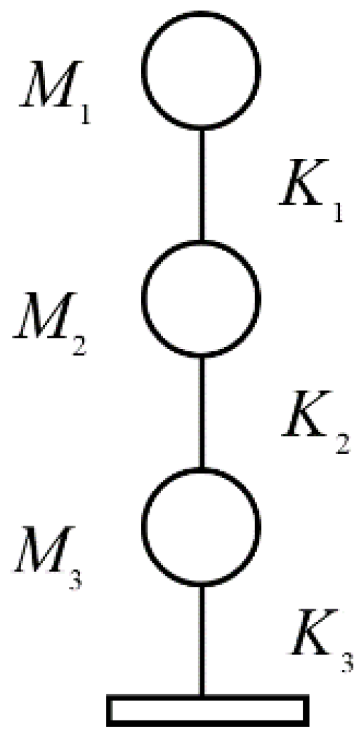
Figure 6.
ACF and PACF of virtual impulse response.
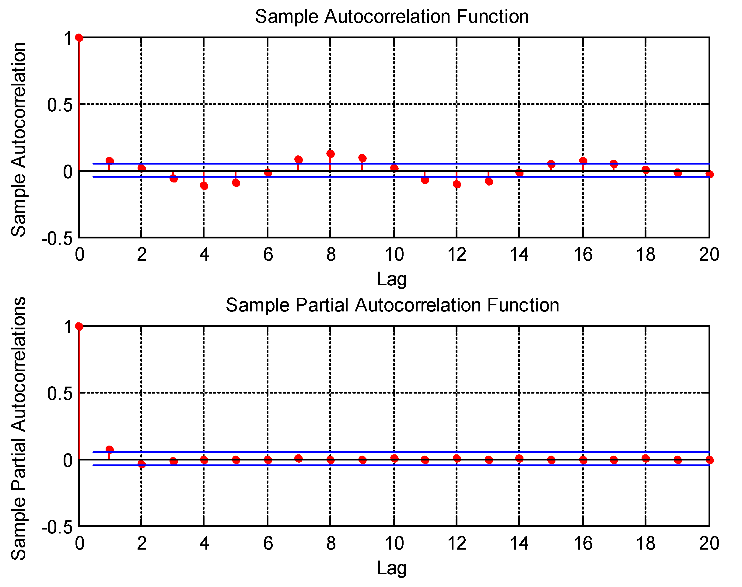
Figure 7.
Ridge regression of coefficient .

Figure 8.
Comparison of AR coefficients in 10 repeated tests under three cases.

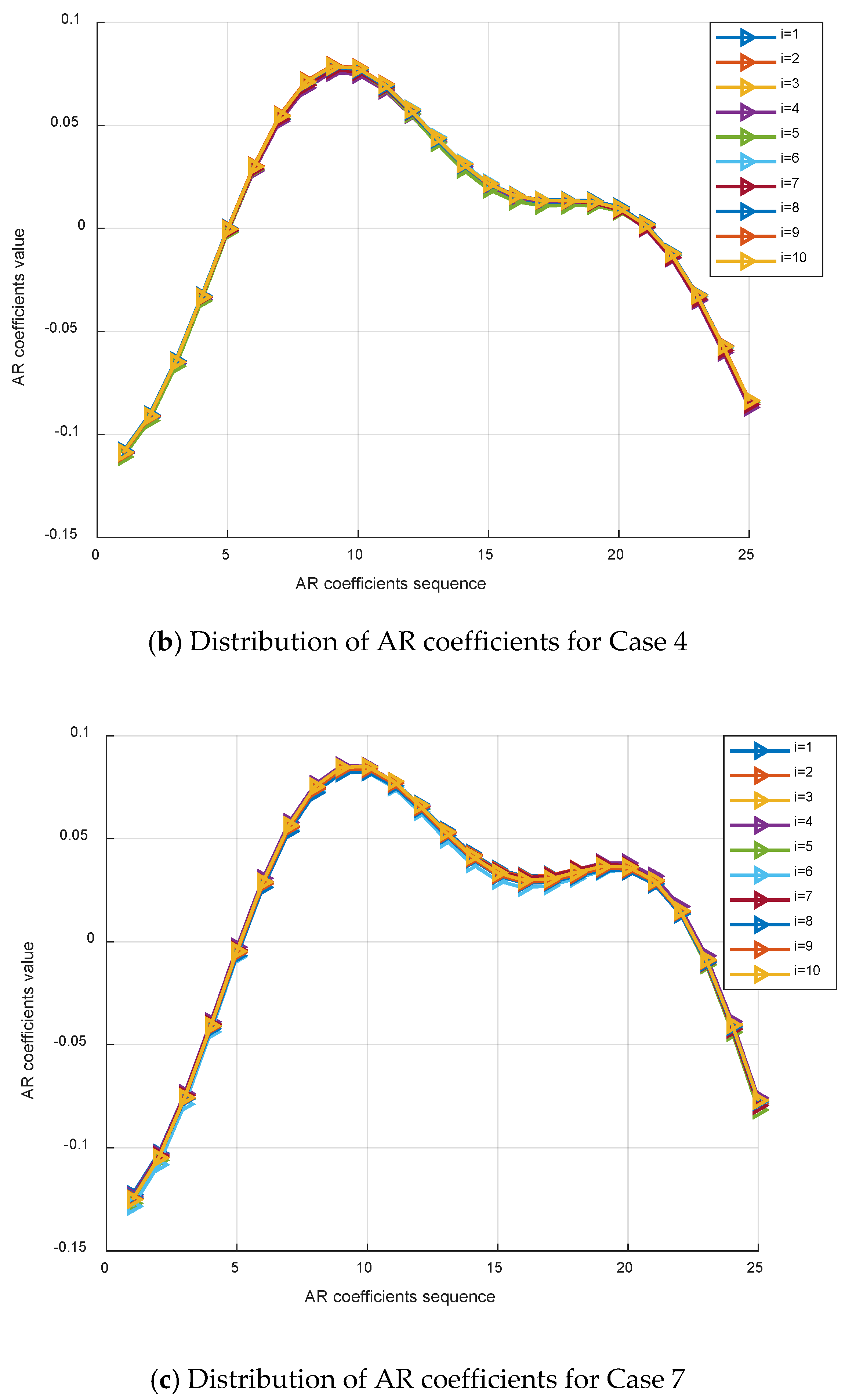
Figure 9.
Damage index DI of seven working cases.
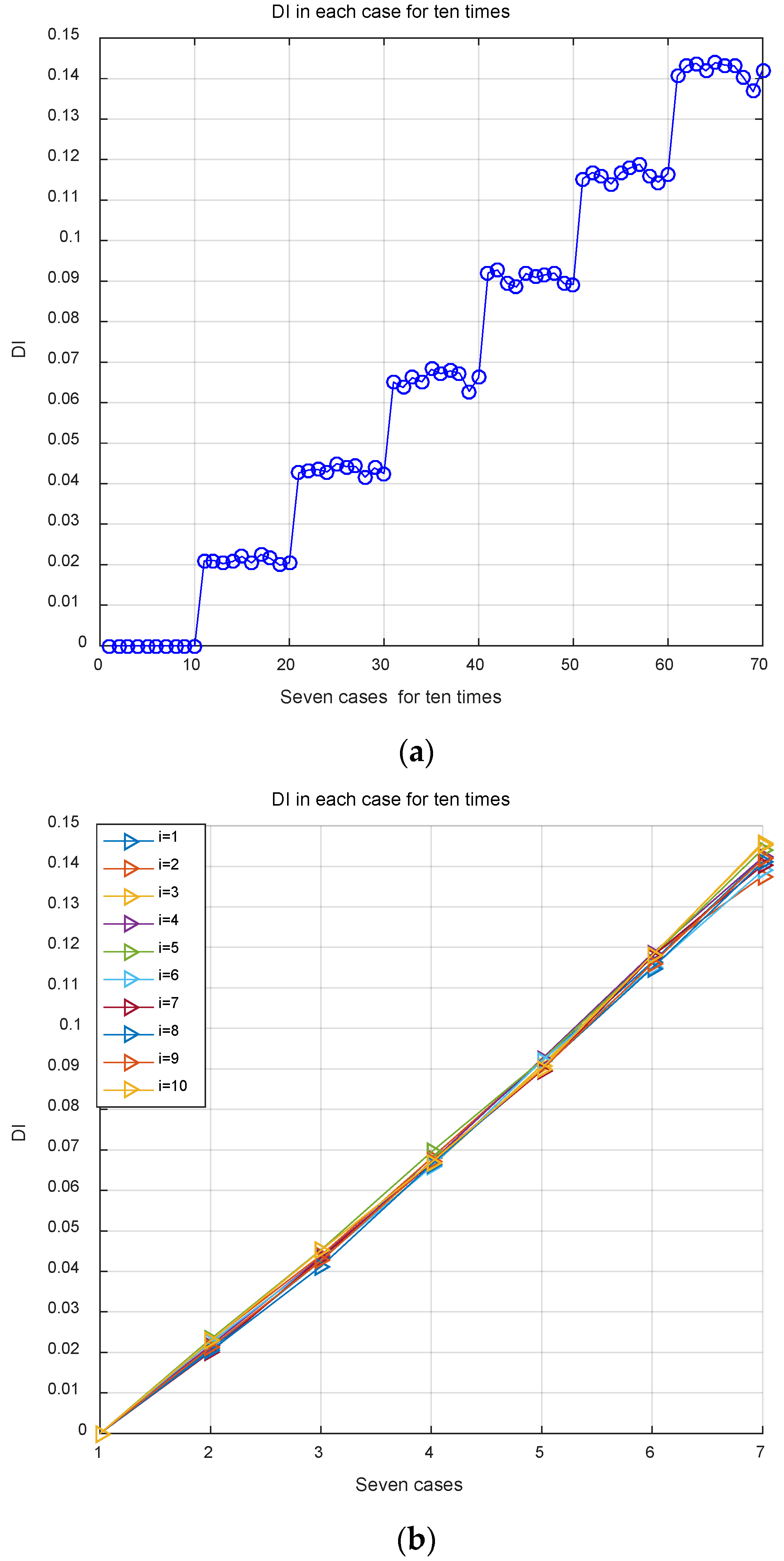
Figure 10.
Test structure setup.
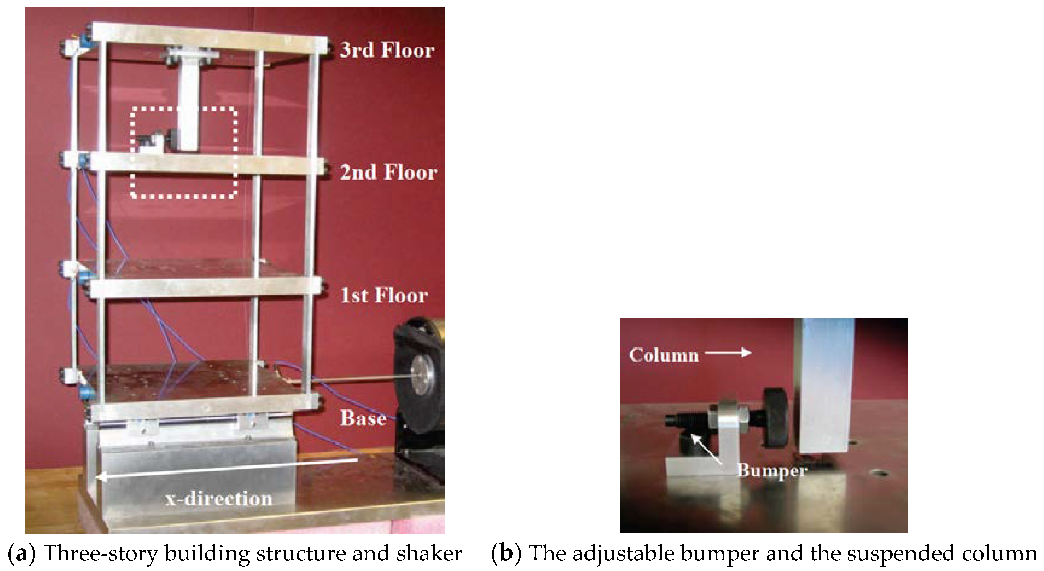
Figure 11.
Basic dimensions of the three-story test bed structure.

Figure 12.
ACF and PACF of virtual impulse response.

Figure 13.
Ridge regression of coefficient .
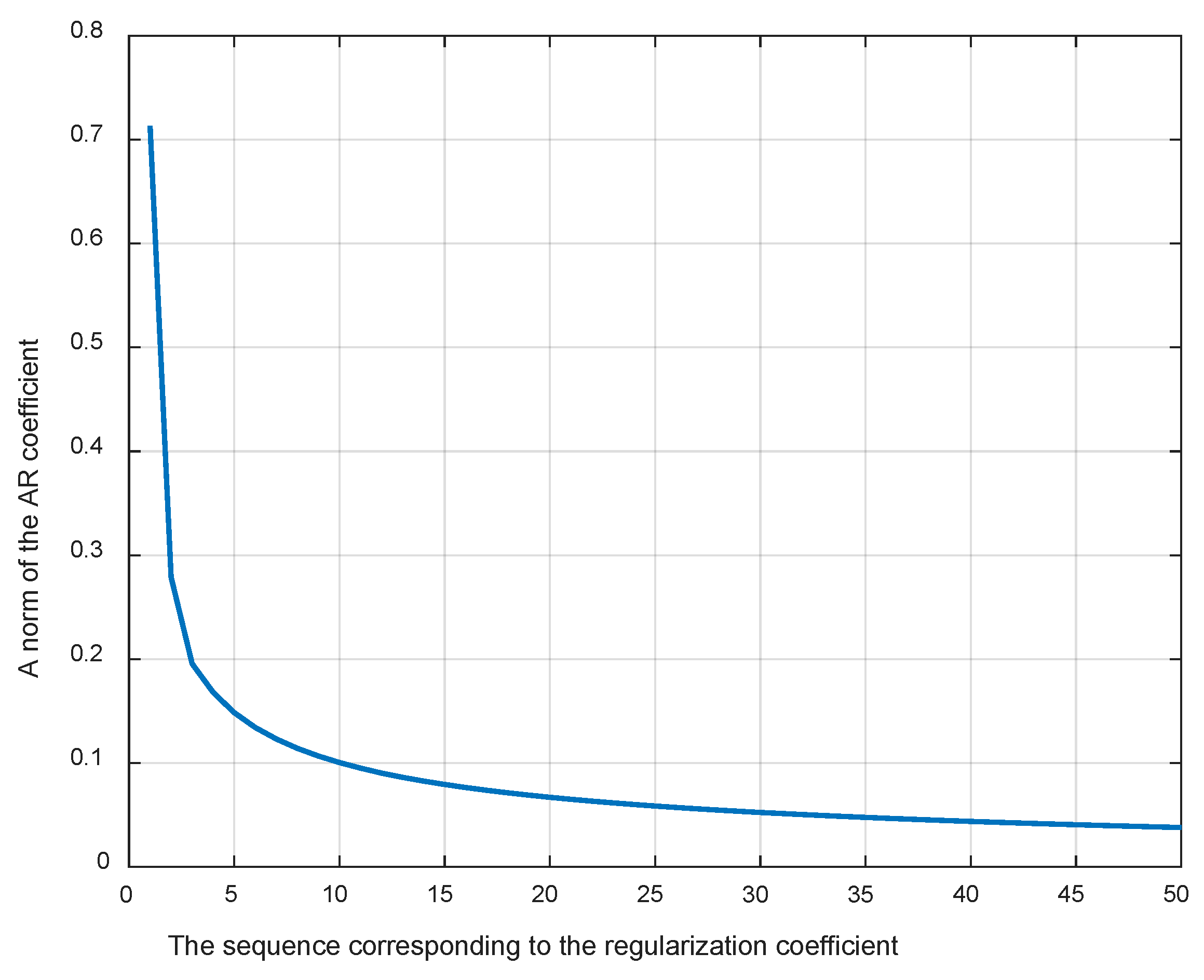
Figure 14.
Damage index DI of five working states.

Table 1.
Damage cases of chain structure with a three-degrees-of-freedom structure.
| Cases | Top Floor Stiffness Reduction Percentage |
|---|---|
| Case 1 | 0% |
| Case 2 | 5% |
| Case 3 | 10% |
| Case 4 | 15% |
| Case 5 | 20% |
| Case 6 | 25% |
| Case 7 | 30% |
Table 2.
Data labels of the structural state conditions.
| Label | State Condition | Description |
|---|---|---|
| State #1 | Undamaged | Baseline condition |
| State #2 | Damaged | 87.5% Stiffness reduction in column 1BD |
| State #3 | Damaged | 87.5% Stiffness reduction in columns 1AD and 1BD |
| State #4 | Damaged | 87.5% Stiffness reduction in column 2BD |
| State #5 | Damaged | 87.5% Stiffness reduction in columns 2AD and 2BD |
© 2018 by the authors. Licensee MDPI, Basel, Switzerland. This article is an open access article distributed under the terms and conditions of the Creative Commons Attribution (CC BY) license (http://creativecommons.org/licenses/by/4.0/).
Share and Cite
MDPI and ACS Style
Zhang, X.; Li, D.; Song, G. Structure Damage Identification Based on Regularized ARMA Time Series Model under Environmental Excitation. Vibration 2018, 1, 138-156. https://doi.org/10.3390/vibration1010011
AMA Style
Zhang X, Li D, Song G. Structure Damage Identification Based on Regularized ARMA Time Series Model under Environmental Excitation. Vibration. 2018; 1(1):138-156. https://doi.org/10.3390/vibration1010011
Chicago/Turabian StyleZhang, Xuan, Dongsheng Li, and Gangbing Song. 2018. "Structure Damage Identification Based on Regularized ARMA Time Series Model under Environmental Excitation" Vibration 1, no. 1: 138-156. https://doi.org/10.3390/vibration1010011