

Convective Density Current Circulations That Modulated Meso-γ Surface Winds near the Yarnell Hill Fire
by
Michael L. Kaplan
1,*,
S. M. Shajedul Karim
2,
Jackson T. Wiles
2,
Curtis N. James
1,
Yuh-Lang Lin
2 and
Justin Riley
2 1
Applied Aviation Sciences, Embry-Riddle Aeronautical University, Prescott, AZ 86301, USA
2
Department of Physics, North Carolina A & T State University, Greensboro, NC 27411, USA
*
Author to whom correspondence should be addressed.
Fire 2023, 6(4), 130; https://doi.org/10.3390/fire6040130
Submission received: 14 February 2023
/
Revised: 21 March 2023
/
Accepted: 22 March 2023
/
Published: 23 March 2023
(This article belongs to the Special Issue Dynamics of Wind-Fire Interaction: Fundamentals and Applications)
Abstract
:On 30 June 2013, 19 Granite Mountain Hotshots firefighters were killed fighting a wildfire near Yarnell in the mountains of Central Arizona. They succumbed when the wildfire, driven by erratic winds, blocked their escape route and overran their location. A previous study is extended to simulate and analyze the downscale organization of convective circulations that redirected the wildfire, which started from the scale of the Rossby Wave Breaking over North America to a convective gust front that redirected the wildfire, trapping the firefighters. Five stages are found: Stage I, the initial deep prolonged gust front; Stage II, a front-to-rear jet and its ascending motions that organized high-based convection; Stage III, high-based dry microburst-induced downdrafts organized initially by ascending flow in Stage II that transported mass and entropy to the surface; Stage IV; multiple meso-γ-scale high centers and confluence zones formed that encompassed the firefighters’ location, which established a favorable environment leading to Stage V, canyon-scale circulations formed surrounding the fire. The atmosphere thus transitioned from supporting a deep and long-lived convective density current to elevated dry microbursts with mass and wind outflow into a canyon, redirecting the ongoing wildfire.
1. Introduction
Entrapments resulting from wildfires typically represent the deadly consequence of local rapidly shifting meso-γ scale winds in complex terrain. Recent well-known wildfire entrapments during the past four years that resulted in firefighter fatalities include the Harris Fire in Joliet, Montana, [1], Devils Creek Fire in Miles City, Montana, [2], and the Carr Fire in Redding, California, [3]. These tragic fires represent the consequence of rapidly evolving atmospheric circulations that are often poorly anticipated or underestimated in operational forecasts. In a recent manuscript by Page et al. (2018) [4], forecasts of wind speed in the gridded National Forecast Digital Database for 2015 were evaluated in fire-prone locations across the conterminous United States during periods with the potential for active fire spread using the model performance statistics of root-mean-square error (RMSE), mean fractional bias (MFB), and mean bias error (MBE). Wind speed was increasingly underpredicted when observed wind speeds exceeded 4 ms−1, with MFB and MBE values of approximately −15% and −0.5 ms−1, respectively. These errors associated with underestimating wind speeds can be deadly in anticipating how local wind can change wildfire behavior. Therefore, the operational firefighting community can benefit from studies of the causes of fine-scale wind bursts and wind shifts that can play havoc with wildfire spread in complex terrain. Such erratic winds and their effects on wildfires are the focal point of this study, which examines a classic example and the complex cause of such phenomena.
The Yarnell Hill wildfire represented one of the most tragic events in the history of firefighting in the United States: more firefighters perished in it than in any fire since the 1930s. In a report released shortly after the tragedy, Karels and Dudley (2013) [5] provided the most comprehensive analysis of conditions associated with this event from the perspective of the USDA firefighting community. Coen and Schroeder (2017) [6], Kaplan et al. (2021) [7], and Ising et al. (2022) [8] have all generated numerical simulations of the Yarnell Hill wind environment leading up to and during the tragedy. The authors of [7] focused on the downscale organization of the environment favorable for the most dominant and long-lived line of convection that developed early in the day over the Mogollon Rim and propagated southwestwards over the Black Hills and Bradshaw Mountains towards Yarnell. Synoptic meso-β-scale circulations, including multiple Rossby Wave Breaks (RWB), terrain-induced frontogenesis, and a mesoscale mid-tropospheric jetlet organized the convective environment sustaining this squall line for >120 km between the Mogollon Rim and Yarnell. This squall line and its leading gust front reached the firefighters approximately 55 min prior to their demise. The authors of [8] performed numerical sensitivity experiments which clarified the relative importance of evaporative cooling, surface heating, and complex terrain structures in the organization of this initial and most persistent convective squall line. More than any other forcing function, evaporative cooling played a key role in gust front maintenance and motion, although the funneling of the outflow and the initial convective triggering clearly were controlled by complex terrain, including multiple successive mountain-plains solenoidal circulations over the Mogollon Rim, Black Hills, and Bradshaw Mountains, and flow blocking by the Weaver Mountains, respectively. These simulations focused primarily on the organization and maintenance of a propagating squall line and its gust front, which approached the firefighters’ ultimate location prior to them being overrun by the wildfire. It should be noted that the National Weather Service Flagstaff Forecast Office utilized a real-time operational model simulation to warn of the likelihood of strong convective outflows creating gusty winds that could affect the safety of the firefighters. The full physics and sensitivity experiment simulations in the studies by [7,8], were however, as was the case of the operational real-time simulation, too coarse to resolve higher-order convective features that subsequently were organized by the primary squall line and its gust front in the immediate hour or less prior to the shift of the wildfire directly into the path of the firefighters. This study employed higher-resolution large eddy simulation (LES) physics to diagnose the cause and significance of convective features organized by that initial squall line minutes before and near the location of the firefighters’ demise. It serves as a precursor simulation study to the actual canyon and fire scale (Δx = Δy < 100 m) simulations with very high-resolution terrain.
Figure 1a depicts the key topographic features in Central Arizona’s high plateau region where the Yarnell Hill wildfire occurred. The four main topographic subfeatures include the Mogollon Rim/Colorado Plateau to the northeast, Black Hills, Bradshaw Mountains, and Weaver Mountains extending to the southwest. The major axis of each of these terrain features is oriented roughly northwest to southeast. The terrain within the meso-γ scale region, including the fire location and Yarnell (Figure 1b,c) is highlighted by a gradually upward-sloping plateau extending southwestwards from Peeples Valley (under the red arrow) towards the Weaver Mountains that wrap around Yarnell from the west to south to east. South and west of the western flank of the Weaver Mountains is a sharp escarpment that descends more than 1 km into the Arizona desert. The eastern flank of the Weaver Mountains bounds Yarnell, as does Peeples Valley to the northeast and north-northwest, respectively, which is bounded by the Bradshaws to the north and east. Thus, Yarnell is surrounded by mountains, and any outflow approaching Yarnell from the Bradshaw Mountains will encounter an ascending valley followed by the Weaver Mountains with numerous fine-scale canyon features <500 m in width and length. Figure 1b highlights the detailed topography and points of interest affecting the firefighters just west of Yarnell. Most significant is the escape route in yellow that the firefighters used in an unsuccessful attempt to reach the safety of the Boulder Springs Ranch. Their final deployment site was in a canyon <500 m in width within the sharply ascending northeastern face of the Weaver Mountains at ~1550 m MSL and ~2 km west of Yarnell. Therefore, they would be exposed to airflow redirecting the fire from the northeast, north, and northwest exiting Peeples Valley in proximity to these mountains. This general northeast–northwest flow direction was observed at ~0000 UTC 1 July at the Peeples Valley and Stanton RAWS surface wind observations shown in [7,8] and tabulated in the validation section below, which represent the only official local surface observation stations.
Figure 2 depicts the evolving perimeter of the fire from 29 June through 1 July from [5] as well as from YHFR (2022) [9]. The fire was triggered by lightning in the hills west of Yarnell on 28 June. One could describe the motion of the fire on 29 June–1 July as having differing stages resulting in large part from the evolving low-level wind fields. For this study, we will describe five different stages of motion. During stage I (29 June into early 30 June), the fire motion was slow and consistent towards the north–northeast moving between 1.5 and 2 km in total. During stage II (1000–1500 MST 30 June), there was a substantial expansion of the fire primarily along its west–east axis as it propagated slightly faster over ~3 km towards the northeast. Dramatic shifts in motion began with stage III (1600–1640 MST 30 June) as the arrival of the primary gust front outflow rotated the fire motion first towards the east–northeast, then sequentially to the southeast, south–southeast, south, and then south–southwest, increasing its speed as it rotated. Stage IV from 1640–1700 MST represents the key period for the danger to the firefighters in which the most dramatic shift is represented by the southwestern perimeter shifting first towards the southeast and then second towards the southwest at a rate of more than several km in 20 min, with a narrow indentation into the canyon depicted as the deployment site for the firefighters in Figure 1b. Finally, Stage V after 1700 MST brought a broad and rapid expansion, primarily towards the southwest in the post-tragedy period. From these motion shifts, one could surmise that an initial southwesterly surface flow was supplanted by a northwesterly flow, then a shift back towards more of a prolonged northeasterly flow as the scale of motion was more focused on the firefighters’ deployment location during Stage IV. This represents three key wind shifts during the period when the firefighters were approaching or within their deployment site, with the most dangerous period ~5–10 minutes before 1700 MST.
Density currents accompanying low-level cold pools are not only ubiquitous convectively generated phenomena but extraordinarily complex in structure. Density or gravity currents launched by moist convective downdrafts and their associated cold pools have been analyzed extensively with far too many studies to reference. However, seminal studies by Charba (1974) [10], Wakimoto (1982) [11], Droegemeier and Wilhelmson (1987) [12], and Liu and Moncrieff (1996a) [13] are important examples that have laid the fundamental groundwork for more recent studies. Most interestingly, analyses in [10] of the boundary layer structure of a density current from tower observations provided insights into just how extraordinarily complex these systems are with staggered arrival of pressure, wind, and temperature discontinuities as well as the complex vertical structure of the hydraulic head, hydrostatic versus non-hydrostatic pressure perturbations, and wind structure accompanying the front-to-rear jet (FRJ). The author of [11] employed Doppler radar to define the four stages of a density current, including what he defined as a precipitation roll phenomenon. Numerical sensitivity studies by [13], Moncrief and So (1989) [14], Liu and Moncrieff (1996b) [15], Xu (1992) [16], and Moncrief and Liu (1999) [17] highlight the sensitivity of density current propagation to environmental conditions, most notably vertical wind shear and stratification. In a very recent study, Luchetti et al. (2020 a, b) [18,19] performed in-depth analyses and idealized simulations of how complex southwestern terrain modifies the motion and intensity of density currents and microbursts. Most notably, their idealized simulations of the interaction of a microburst outflow and canyon highlight the importance of microburst proximity to eventual complex canyon circulations.
For this Yarnell case study, studies by Weckworth and Wakimoto (1992) [20], Jin et al. (1996) [21], Wilson and Megenhardt (1997) [22], Weismann and Rotunno (2004) [23], Siegel and Van Den Heever (2012) [24], Bryan and Rotunno (2014) [25], Reif et al. (2020) [26], and [18,19] are particularly prescient; however, our concern is how the density current triggered secondary and tertiary circulations such as the FRJ and microbursts in complex terrain that impacted the surrounding environment. The authors of [20] diagnosed the importance of Kelvin-Helmholtz instability in the convective initiation process above the density current head. This instability and its associated internal gravity waves played a key role in subsequent convection above a gust front, all of which were diagnosed from Doppler radar observations. The authors of [21] employed multi-scale observations and idealized numerical simulations to analyze the gravity waves generated by a density current in an atmosphere with complex vertical stratification. Lee wave and Kelvin-Helmholtz waves with varying wavelengths were launched in the neutral layer with a substantially curved environmental vertical wind profile above a propagating density current. The waves above the FRJ were primarily evanescent and wavelength depended upon their elevation. The authors of [22] demonstrated the importance of density current propagation relative to the airflow vector 2–4 km above the current. When this direction was in the same direction as the density current motion, longer-lived convergence and convection could be sustained during a Florida sea breeze. The authors of [23,24] performed idealized simulations indicating that the longevity of the current and its optimal maintenance of convection was facilitated by a balance between baroclinically generated vorticity and vertical wind shear as well as the slope of the leading edge of the current. The authors of [25] performed idealized numerical sensitivity studies to diagnose the relationship between the speed of density current motion and the height of the inversion layer above the current. This sensitivity was strongly dependent on the inversion depth in so much as whether it acted as a gravity wave duct or not. Thinner stable layers that could not support ducted gravity waves acted to accelerate the speed of the gravity current. Finally, [26] employed observations from PECAN to diagnose the conditions that led to an optimal vertical velocity at the density current head. They formulated an equation in which the optimal angle of the density current relative to the ground was directly related to the vertical velocity, thus better facilitating convective initiation. Angles ~40–50° were far more effective at generating large vertical velocities than smaller angles. Thus, extensive observational and numerical simulation evidence confirms that a density current is fully capable of organizing additional convective circulations and complex wave/jet phenomena.
This study tested the hypothesis that the forcing by an extraordinary fast-moving, deep, and long-lived density current, its leading ascent, FRJ, and its initiation of high-based convection and subsequent microbursts were critical to the wind fluctuations at Yarnell minutes before the death of the Prescott Mountain Hotshots. The density current’s convective initiation resulted in a sequence of microbursts or shafts of rain-cooled air that mostly evaporated before reaching the surface. It will be shown that this was an extraordinarily deep and fast-moving density current with a very strong leading ascent zone and well-organized FRJ that interacted with subsequent rain-cooled plumes of descending air. The environment favored this type of current as it was quite representative of the Southwestern United States during hot weather above elevated terrain. A deep, dry, neutral well-mixed planetary boundary layer (PBL) exceeding 3 km above the elevated plateau of ~1.5 km MSL was capped by a stable layer extending several km above the tropopause. The primary moist layer was elevated between 600 and 300 hPa above a dry PBL. This structure is quite different from that of most of the published case studies as the downdraft convective available potential energy (DCAPE) was very large, consistent with favorable environments for relatively dry microburst phenomena, and the neutral PBL was capped by a very deep stable layer that was deep enough to duct internal gravity waves.
Microbursts of the wet and dry variety are well-studied phenomena: numerous observational and numerical studies have been published, including those by Wilson et al. (1984) [27], Wakimoto (1985) [28], Fujita (1985, 1990) [29,30], Proctor (1988) [31], Hjelmfeldt (1987, 1988, 2010) [32,33,34], Elmore et al. (1986) [35], and Roberts and Wilson (1989) [36], as well as many more. Clearly, the Yarnell Hill wildfire environment, with very large DCAPE consistent with a deep dry neutral and hot PBL under a moist mid-upper troposphere and with elevated most unstable convective available potential energy (MUCAPE), favored relatively dry microburst phenomena. As will be shown later, the classic dry microburst inverted V-shaped sounding, including a deep neutral layer and extreme DCAPE, existed minutes before the Yarnell Hill Fire was redirected towards the Hotshots’ location in Figure 1c; i.e., the deployment site.
Thus, in this study, we will describe how the wind fluctuations near the canyon where the Hotshots were camped were directly relatable to the interaction among the primary density current, its lifting, its FRJ, microbursts, and complex resulting circulations that affected their canyon encampment. In the remainder of this study, Section 2 will describe the assumptions employed in the multiply nested grids in the very high-resolution numerical simulations that were used for the analyses. Section 3 will briefly describe what radar and surface observations exist in the region of interest to validate the very high-resolution simulations and the strengths and weaknesses of the high-resolution simulations based on these validation datasets. In Section 4, the following components of the key simulated circulations, as they arrived in the region of the fire that influenced the local wind flow, will be analyzed in depth: (1) the primary density current structure and circulation, (2) the elevated convection and its attendant microbursts’ structure, and (3) the deposition of mass in the PBL by the microbursts and FRJ and how they combined to create complex and remarkably sustained low-level flow consistently directed towards the Hotshots’ deployment site, where they perished. We speculate that the exceptionally prolonged nature of the low-level northeasterly flow, and possibly also its very strong low-level shear, were the key contributors to the firefighters’ demise. Section 5 will involve a detailed summary and conclusion as well as a description of future work.
2. Methodology
The Weather Research and Forecasting model ARW version 3.6.1 was utilized for the numerical simulations for the first 3 grids (d01–d03) as in [7,8], while the WRF-LES version 4.4 was utilized for grid d04 (Skamarock et al. 2004, 2008, 2021) [37,38,39]. The initial and largest domain lateral boundary conditions employed the European Centre for Medium-Range Weather Forecasts Reanalysis 5 dataset (ERA5) (Hemri et al. 2022) [40]. ERA5 is available every hour for most variables and has global coverage with a spatial resolution of approximately 30 km and 137 vertical levels from the surface up to a height of 80 km. The simulation domain was set up with a 3:1 ratio on a Lambert conformal map projection starting at a horizontal resolution of 7 × 7 km as the outermost domain (d01), then 2.33 × 2.33 km as domain 2 (d02), and 0.777 × 0.777 km as domain 3 (d03), as shown in Figure 3a. D01 extends from California to Arkansas and from Wyoming to Texas. D02 extends from approximately Baja California to Central Texas and Utah to Central Texas. D03 covers most of the state of Arizona and is approximately centered over the Yarnell Hill Fire. D01 and d02 were extended toward the north and east of Arizona to capture the synoptic setup to allow for spin-up time and to capture the convection passing through the lateral boundaries. D01 started on 29 June 2013, 1700 MST (30 June 2013, at 0000Z), and ended on 30 June 1700 MST (1 July 2013, at 0000Z), since that was just after when the Yarnell Hill Fire incident occurred. Each subsequent domain started and ended on the same days but at later start times (0500 MST/1200Z for d02 and 0800 MST/1500Z for d03) and the same end time. One-way grid nesting was utilized for d02–d03 with time-dependent boundary conditions from the coarser grid. For the vertical resolution, 50 stretched levels were used on all domains. Land use data were taken at 5 arcminutes (d01), 2 arcminutes (d02), and 30 arcseconds (d03) from the MODIS IGBP 21-category dataset. In meters, 5 arcminutes are about 7600 m, 2 arcminutes are about 3000 m, and 30 arcseconds are about 760 m, for a latitude of 34.22° N (Yarnell, AZ). Output was written every 4 h (d01), 1 h (d02), and 15 min (d03).
For the grids in the WRF-ARW simulation (d01–d03), the Purdue–Lin scheme (Chen and Sun 2002) [41] was used to represent microphysical processes. For the surface, land surface, and boundary layer physics schemes, the Eta similarity scheme (Monin and Obukhov 1954 [42]; Janjic 1994, 1996, 2002 [43,44,45]), unified Noah land-surface model (Tewari et al. 2004) [46], and Mellor–Yamada–Janjic (Eta) TKE (Mesinger 1993 [47]; [43]) were used. The cumulus parameterization was set to the Grell–Freitas ensemble scheme (Grell and Freitas 2014) [48] only for the outermost domain (D01), since this scheme is scale-sensitive at a horizontal domain resolution of 7 km. For all other domains, no cumulus parameterization scheme was used. These physics, in general, were chosen to include parameterizations that are not too computationally expensive but still representative of the convection and the wind event. The Purdue–Lin scheme was chosen because it is a five-class microphysics scheme that includes graupel and because of its ability to handle high-resolution domains. The Eta similarity scheme was chosen because of choice for the boundary layer physics scheme (paired), the unified Noah land-surface model because of its sophisticated vegetation modeling, and the Mellor–Yamada–Janjic (Eta) TKE scheme for its ability to handle thin layers. Figure 3b depicts the 900 m topography for d01–d03 as well as soundings, horizontal zoomed-in region, and vertical cross-sections.
WRF-LES version 4.4 was employed for the d04 259 m nested grid initialized from d03 at 2200 UTC (1500 MST) and run until 0000 UTC with time-dependent boundary conditions from the d03 grid with the same number of vertical levels, microphysics scheme, and land-surface formulations as d03, and the same carried down through d04. A horizontal grid spacing of 250 m has been shown to be adequate to resolve the inertial subrange and for LES subgrid-scale closures to sufficiently perform as designed (Bryan et al. 2003 [49]; Lebo and Morrison 2015 [50]). Terrain data employed for the d04 simulation is depicted over the enlarged region near Yarnell in Figure 3b. This 259 m simulation employed relatively smooth 900 m resolution terrain. Future simulations at the canyon scale (<100 m resolution) employed terrain derived from the Shuttle Radar Topography Mission 1 arcseconds (30 m) dataset (SRTM1; details can be found at http://www2.jpl.nasa.gov/srtm/, accessed on 15 October 2022). The d04 simulation was designed to diagnose the convective density current and its secondary circulations, which will subsequently be employed to provide initial data for higher-resolution WRF-LES and WRF-FIRE simulations in the future. The domain configuration of the WRF model, physics parameterization schemes, and dynamics employed for this study are summarized in Table 1.
Radar analysis for model validation was performed using software called GR2Analyst v3.0.2.3, created by Gibson Ridge Software, LLC, Suwanee, GA, USA. It enables the visualization of full-volume WSR-88D radar data. The TFSX radar data were exclusively employed due to the non-availability of the TPHX and TYSX radars.
3. Validation
Validation of the 259 m simulation was derived from subjective radar inter-comparisons and direct RAWS observations at Stanton and Peeples Valley (see Figure 3b for locations). Table 2 depicts a comparison among the observations at the Peeples Valley and Stanton RAWS versus the 259 m simulation. Figure 4 depicts key TFSX Doppler radar reflectivity features from 2247–2348 UTC, while Figure 5 depicts the 259 m simulated radar reflectivity and 10 m wind barbs from 2315 UTC–2355 UTC. From Table 2, it is clear that while the 259 m simulation compares favorably to the Stanton RAWS, it does very poorly when compared to the Peeples Valley RAWS.
The location of the microburst-induced convective outflow likely represents the primary source of error in terms of surface wind and temperature fields at the Peeples Valley location. This error is apparent when we compare the model-simulated radar reflectivity in Figure 5 to the observed reflectivity from the TFSX Doppler radar in Figure 4. The model misplaced the microburst convective cells slightly (~2 km) too far to the west and likely aliased too large a scale, creating a convective outflow signature in the surface winds that turns the observed northeasterly flow to the southeast and accelerates it dramatically at the Peeples Valley location. This appears to overwhelm the observed flow at Peeples Valley. However, at Stanton, somewhat more displaced from the microburst convective outflow, the winds and temperatures are very similar between the model and observations, albeit representing poor resolution in time due to the limited number of observations. At Stanton, we also see confirmation of the primary density current passage with a strong northeasterly wind shift and temperature drop at 0001 UTC. This can also be compared to Figure 6, where the density current windshift, pressure rise, and temperature gradient features viewed in two-dimensional space can be seen and will be described in greater detail in the next section. The model does simulate the three most important meso-γ-scale convective features, including (1) the sharp, rapidly propagating primary density current validated at Stanton and through observations from numerous observers (e.g., [5]), (2) newly developing cells over the northeastern part of the grid accompanying the density current and subsequent microbursts and their secondary outflow regions, and (3) another (parallel) zone of convection along the eastern Weaver Mountains with some degree of similarity to the observations. Most notably, the windshifts and cooling at the RAWS close to the observed time, and new convection propagating from the northeast to the southwest into the deployment location of the Hotshots are simulated, albeit with some anticipated error, given model imperfections and the omnipresent imperfection in the d01 initial conditions. This model-generated convection closely approached Yarnell and the Hotshots’ location in the simulation and rapidly weakened, not unlike the observed convection. This weakening of convection is not surprising due to the deep dry environment over and southwest of the western flank of the Weaver Mountains.
A closer comparison of the model simulated reflectivity in Figure 5 with (1) the horizontal plan position indicator (PPI) display over Central Arizona, (2) zoomed-in displays of the reflectivity centered just northeast of Yarnell, as well as (3) vertical cross-sections of reflectivity from Spruce Mountain within the Bradshaw Mountains to the location of the Hotshots (YHFT) in Figure 4 is important to show subjective model validation. Like the observations, the model indicates developing 25–30 dBz cells spreading southwestwards but just slightly northwest of the observed 25–30 dBZ reflectivities in Figure 4c–g roughly parallelling Arizona state route 89 (orange line in Figure 4g) between Yarnell and the Bradshaw Mountains starting shortly after 2310 UTC. The model-focused grid region displays secondary convection accompanying the density current, which is not the original squall line. That original line propagated all the way from the Mogollon Rim to the western slopes of the Bradshaw Range is denoted as the dying >50 dBz hail core in Figure 4a,b. This original convection can be seen to be weakening in the subsequent Figure 4 displays as well. Within the observations are clear signals of the elevated nature of the convection with cloud bases ~3 km MSL above the elevation sweep of the TFSX radar of ~2500 m. Also shown is a likely indication from the vertical reflectivity cross-section of the cells building down from nearly 10 km MSL to lower elevations (Figure 4a,b) during the incipient period of the primary density current spreading southwestwards through Yarnell. This period is very interesting because, consistent with the primary density current moving through Yarnell and the filling in of echoes, the smoke plume just northwest of Yarnell makes a rapid shift to the south–southwest in Figure 4f consistent with Figure 2 from [5] and Figure 21 in [7]. The filling-in of echoes in the radar roughly above Peeples Valley is closely aligned in time with the model being slightly west of the observed convection and as will be shown in the next section, this filling-in is consistent with the density current lifting above its hydraulic head and the strengthening of the FRJ upstream of Yarnell. Of particular interest from the TFSX Doppler in Figure 4g in the 1.3° elevation scan are the zoomed-in base reflectivity fields at 2335 UTC showing an enhanced cell just NNW of Yarnell and line of developing convection at 2339 UTC extending west–northwestward from Yarnell in the broader scale PPI. As the model generates stronger embedded echoes just west–northwest of the observed in Peeples Valley by 2330 UTC, it also spreads the higher-elevation lower-dBZ echoes southwestwards consistent with the TFSX radar. The TFSX radar in Figure 4f,g is also proof of a companion area of convection just to the east over the eastern flank of the Weaver Mountains and Yarnell, which is captured in the model. The simulated convection evolves into a weakly bowing echo ahead of the microbursts, not unlike the observed radar signal. The TFSX radar vertical cross-sections in Figure 4h–j indicate that while the convection was not very intense, cell tops rapidly increased in elevation and reached above 14 km MSL after 2338 UTC near the Hotshots’ location at the southwestern end of the vertical cross-section from Spruce Mountain in the Bradshaw Range to YHFT. Therefore, vertical motions were likely very significant in the mid-upper troposphere, which we will see later is consistent with the elevated MUCAPE-generated convection above the primary density current’s hydraulic head and deep FRJ.
4. Simulated Meso-γ-Scale Convective Circulations in Peeples Valley
4.1. Primary Density Current Acceleration and FRJ Formation
Figure 6 depicts staggered 5 and 10 min wind, mean sea level pressure, and temperature fields that denote the arrival of the primary density current within the 259 m simulation’s grid and its expanded southwestern grid region (Figure 3b) from 2250–2355 UTC. Figure 7 depicts the vertical cross-section C-D’s (Figure 3b) 3D wind vectors and potential temperature of the density current and multiple convective cells and their downdrafts during the same time period. These latter two figures show the broad area of the two-dimensional primary density current propagation followed by the isolated cross-section region from ~10 km northeast to ~5 km southwest of the Hotshots’ location, focusing on Peeples Valley and the western flank of the Weaver Mountains. The period 2245–2315 UTC is the time during which the density current travelled very rapidly ~15 km from roughly the northeastern part of Peeples Valley to the foothills of both flanks of the Weaver Mountains. At 2315 UTC, the density current was just southwest, south, and southeast of the Hotshots’ final deployment location. This density current (note black cold frontal symbols in Figure 6a–c) far outraced its parent convective line, which slowly dissipated as it propagated southwestward down the Peeples Valley from the Bradshaw Mountains (Figure 4a–d). In the horizontal depiction in Figure 6a–c, as the wind shift approached the Hotshots’ location, note that the wind shift/convergence zone was roughly in phase with the hydraulic head, HH in Figure 7a–e, as inferred from the rising mean sea level pressure and then its closely trailing temperature-fall field in a manner not unlike that described in [10]. In other words, like Charba’s observations, the wind shift and non-hydrostatic pressure rise were closely coupled with the larger-scale temperature fall, while the broader hydrostatic pressure rise zone accompanying a meso-high was located directly under the dry microbursts’ mid-upper tropospheric raincooled air, which was trailing upstream.
Figure 7a–f’s cross-sections clearly depict the strength of the density current’s (DC) hydraulic head (HH) and wind shift displayed in the horizontal cross-sections in Figure 6a–c. Figure 7a–f also depicts multiple very high-based convective cells and a robust northeastward-directed mid-tropospheric FRJ centered early on above the density current cold pool at ~650 hPa that descended through the simulation. The simulated velocity of the leading edge of the wind shift accompanying the density current varied substantially at 5 min intervals, as derived from the location of the hydraulic head in Figure 7a–f. The maximum simulated horizontal velocity of the moving head was ~17 ms−1 between 2250 and 2255 UTC, ~14 ms−1 between 2250 and 2300 UTC, ~10 ms−1 between 2300 and 2305 UTC, ~7 ms−1 between 2305 and 230 UTC, and ~7 ms−1 between 2310 and 2315 UTC. The extraordinary variability and generally high rate of speed reflect the changing depth of the density current head and the streamwise temperature gradient across the head in its forward direction of motion. During its maximum velocity period, the depth of the head approached 1 km as it extended above 750 hPa into the deep well-mixed PBL, as can be seen in Figure 7, while the streamwise potential temperature gradient exceeded a remarkable 5 Kkm−1 along its leading edge at times in Figure 7. Given the maximum velocity, this represents a sharp local temperature fall in a few minutes. The hydraulic head and temperature gradient represent very strong features which, to a large extent, reflect the extreme heat in Peeples Valley at the surface. This heat, more than 40 °C, as can be seen in Figure 6a–c, was located relative to the cold pool propagating down the Bradshaw Range’s southwestern slopes into Peeples Valley as forced by the >50 dBZ hail core downdraft, and its evaporational cooling inferred accompanying the dying squall line from Figure 4a–d. To verify that such high velocities of motion were consistent with density current theory during its maximum velocity, we employed the early period density variation across the head, height of the head, and potential temperature variability across the head to calculate the theoretical velocity from two different formulas depicted below in Equations (1) and (2) from [10] and [18], respectively. Here, K = Froude number in our data ~0.7, D is the depth of density current, g is gravity, ρ2 and ρ1 of the ambient and density current air, respectively, θ and θ′ are the potential temperatures of the ambient and density current, respectively. K was calculated from the simulated data. Both equations confirm maximum theoretical propagational velocities ranging from ~20–22 ms−1, which is ~10–20% faster than the simulated maximum velocity between 2250 and 2255 UTC and subsequent slower values when the temperature gradient along the stream weakened thereafter. Perhaps simulated surface friction is responsible for the difference? This deep, rapidly moving, and long-lived density current will produce very large ascending motions consistent with a large angle >45° between the sloping head and the ground and thus transfer substantial mass vertically as well as in the upstream direction (e.g., [24]).
The northeastwards-directed FRJ was embedded in a neutral layer that contained lee wave-like structures that have a wavelength generally ranging between 5 and 10 km. The wavelength is consistent with a vertically decreasing Scorer parameter profile in the mid-tropospheric, neutrally stratified layer that contained the FRJ analogous to the study of [20,21]. The Scorer parameter variation reflects the curvature of the FRJ wind profile in the vertical as well as the low values of Brunt-Vaisalla frequency within the deep neutral layer that contained the FRJ. Horizontal wind velocities directed upstream towards the northeast in the plane of the vertical cross-section in Figure 7 and Figure 8 exceeded 16 ms−1 in the neutral shear layer, roughly between 500 and 700 hPa for much of this time period. The total distance encompassed by the FRJ exceeded 10 km; therefore, affecting the horizontal extent of most of Peeples Valley up to the foothills southwest of the Bradshaw Mountains, as can be seen in the later panels in Figure 7. Numerous vortices (rotors) developed in conjunction with the waves in viscous surface flow, as described in [20] and Doyle and Durran (2002) [51]. This FRJ represents an extremely strong countercurrent to the motion of the density current and will be shown to represent another source of mass and enhanced vertical wind shear to be transported surfacewards after the mostly dry microbursts formed and slowly descended at a later time northeastwards along the vertical cross-section.
4.2. Microbursts and Thermodynamic Structure above the FRJ
During the period between 2305 and 2320 UTC, noted earlier, a northeast–southwest line of high-based convective cells can be seen in Figure 4 and Figure 5 rapidly developing above the observed propagating density current, which is similar to the one in the 259 m simulation depicted in Figure 6. It should be emphasized that the cells only developed once the density current propagated across most of this region just after 2311 UTC, as can be seen in Figure 4e–f. We say high-based in that the TFSX radar is located at nearly 2500 m MSL and thus only sees a relatively upper-level/elevated hydrometeor signal well above 750 hPa. The primary elevated cells can be inferred from the 259 m simulation in Figure 7b,d, in which >20 ms−1 ascending flow develops within the plume of maximum vertically varying mass flux convergence, above mid-level mas flux divergence, with the maximum ascent centered within the 250–350 hPa layer at 2315 UTC. This first cell (C1) only develops about 10 min after a vertically propagating gravity wave penetrates through this layer with nearly the same vertical motion values near the 10 km location. This strong ascent moistens the upper troposphere above the MUCAPE within the mid-tropospheric neutral layer over Peeples Valley along cross-section C-D. A second cell (C2) follows to the southwest near the 8 km location a few minutes later in Figure 7. The early vertically propagating gravity wave was directly above and coupled to the rapid lift above the density current’s hydraulic head and explosively developing FRJ. Later descending mass flux maxima developed to the northeast near the surface along cross section C-D in Figure 8d–f.
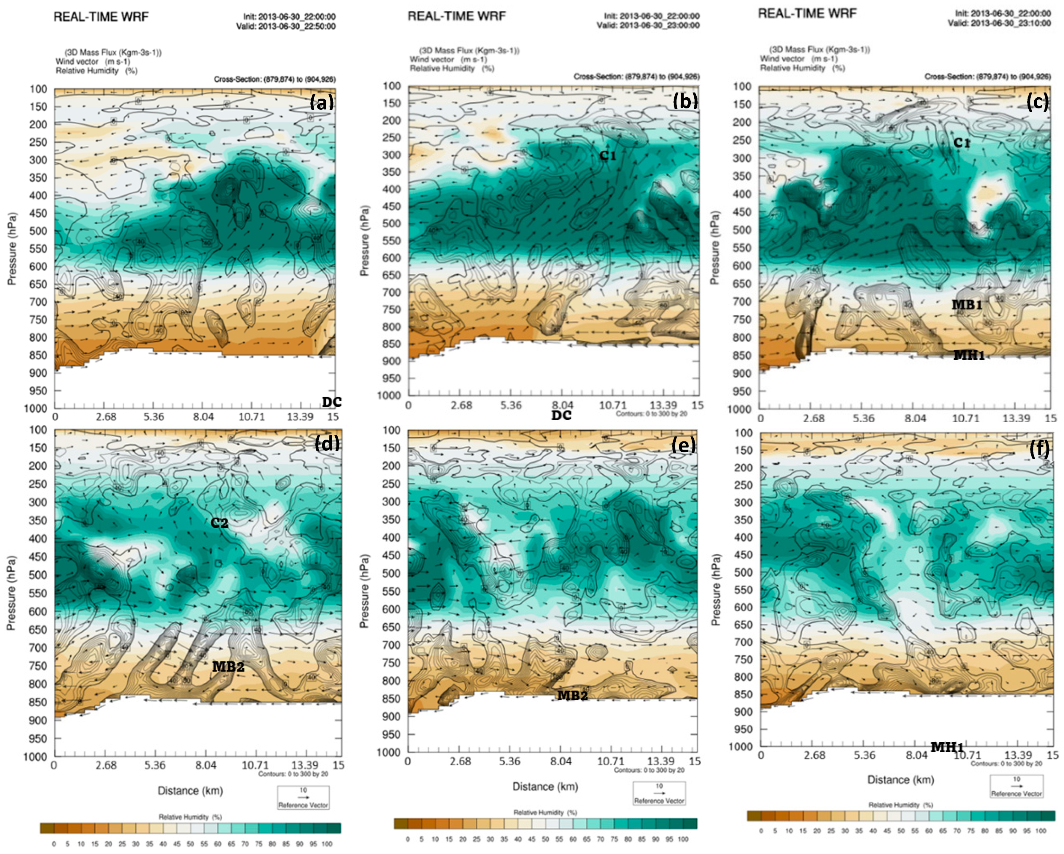
Figure 8 depicts the 3D mass flux convergence, 3D winds, and relative humidity along cross-section C-D during this important time period for the region just upstream from (northeast of) the Hotshot’s deployment location extending beyond 2250 UTC, i.e., out to 2340 UTC. Above the hydraulic head is an exceptional plume of mass flux convergence in Figure 8a–c near locations 13, 8, and 2 km along the cross-section. These maxima were being transferred vertically, forming and maintaining the incipient FRJ within the plane of the cross-section from 2250–2310 UTC. These mass perturbations propagated above the stably stratified layer, capping the well-mixed PBL upstream away from the head over the period from 2250 to 2340 UTC near 650 hPa. They contributed to the vertical mass flux in the updraft for the first and second elevated convective cells. In Figure 8, one can see the following: (1) mass flux convergence near the surface coupled to the hydraulic head, (2) trailing mass flux convergence upstream under dual cells that produced subsequent dry microbursts, (3) remarkably varying mid-tropospheric mass flux convergence in the upper troposphere indicative of the effect of multiple high-based convective cells (C1–C2) in the wake of the head, and (4) a strong FRJ transporting mass upstream for most of the period centered near 650 hPa and descending later in time. This latter plume of mass and momentum within the neutrally stratified mid-tropospheric layer above the cold density current air is apparent in Figure 7 and Figure 8, as is the increased northeastward-directed flow in the FRJ centered near 650 hPa that was forced to descend multiple times under the influence of the high-based convective cells and underlying dry microbursts. C1 was near location 10 km and C2 near location 8 km between 2300 and 2315 UTC in Figure 7 and Figure 8. Dry microbursts followed these cells, as can be inferred from Figure 5, Figure 6, Figure 7 and Figure 8. In Figure 5b–d and Figure 6e,f, the MD and H symbols denote the surface diffluence and meso-high formations in horizontal space accompanying relatively cool surface air in proximity to the upper region of cross-section C-D in Figure 7e–g,k,l. Expanded isentropes and downward directed 3D wind vectors in these figures signal low-level cooling and descending rain-cooled air parcels, generally between 700 and 800 hPa, that comprised the dry microbursts. In Figure 8c,f, local mass flux convergence near the surface reflects the cooling and sinking motion that expanded in scale upstream and towards the end of the simulation.
Nine soundings from the 259 m simulation at 10 min intervals between 2300 and 2320 UTC were generated and are displayed in Figure 9. They indicated a maximum MUCAPE > 400 jkg−1 early during this period and also exhibit a maximum DCAPE > 1000 jkg−1 within the moist mid-tropospheric upper part of that neutral layer capping a dry lower troposphere. Elevated MUCAPE generally existed between 700 and 500 hPa as the lifted condensation levels (LCL) were generally just below 600 hPa. The sounding locations (#1, #2, and #12) are depicted in Figure 3b. These are classic v-shaped high-elevation soundings that are often associated with high-base moist convection in complex terrain, as can be supported by much of the aforementioned dry microburst literature [31]. Typically they contain high-level LCLs and levels of free convection (LFCs) within a very deep adiabatic layer. Figure 9 depicts soundings 1, 2, and 12 located in Figure 3b at about the time convection was triggered and propagated southwestwards in Figure 4 and Figure 5 in response to the density current lifting discussed earlier, i.e., during 2310–2330 UTC. What is very interesting about this sounding intercomparison is that sounding 12 had relatively large MUCAPE for this type of dry elevated convective environment, moderate CIN, and moderate precipitable water, yet full saturation in the 400–550 hPa layer occurred primarily in soundings 1 and 2 for several 5 min sequential periods but at no time in sounding 12. The difference being soundings 1 and 2 were associated with somewhat larger vertical wind shear and vertical mass fluxes at mid-levels as a result of the density current-driven FRJ. The FRJ influence in which an opposing mid-tropospheric west–southwesterly flow sharply undercut the background upper-tropospheric east–northeasterly flow accompanying a mesoscale jetlet, described in [7], did not occur to a similar magnitude at sounding 12’s location to the east–southeast of the density current lifting. The contrast with soundings 1 and 2 is also interesting, where much weaker MUCAPE and larger CIN existed relative to sounding 12 but saturation still occurred in response to density current-induced shears and the vertical mass fluxes accompanying a favorable non-hydrostatic ascending environment deep into the upper troposphere. These two soundings (#1–2) were the closest to the simulated high-based convective cells that organized descending plumes of air in concert with the FRJ northeastward along vertical cross-section C-D. These soundings are typical of dry microbursts [28,29,30,31,32,33,34,35,36].
A strong ascent accompanying a vertically propagating gravity wave in Figure 7b at 2255 UTC occurred immediately prior to moist convection. This ascent enhanced the background moist environment for the high-based primary dry microburst and subsequent dry microbursts, which can be seen above the hydraulic head in the upper troposphere. The ascent moistened the mid-upper tropospheric layer, thus allowing high-based parcels to reach their elevated LFCs of ~550 hPa in Figure 9. The dominant cell near sounding #2 and along cross-section C-D east–northeast of Peeples Valley quickly dissipated after 2320 UTC with 3D vectors indicating upper tropospheric sinking that continued for nearly 25 more minutes through 2345–2350 UTC into the air that was substantially subsaturated. Figure 8 depicts cross-section relative humidity during this time period indicating the change from moist adiabatic and initially saturated to dry adiabatic and terminally unsaturated descent as air parcels reached and diverged outward within the PBL as cold pools in association with dry microbursts. Shifting along a cross-section northeasterly flow signals this surface divergence in Figure 7. Parcels descended at >5ms−1 towards the surface, thus penetrating the neutral layer, FRJ, and cool residual air within the density current along cross-section C-D ~5–10 km northeast of the Hotshots’ deployment location during this critical time period between 2325 and 2345 UTC.
4.3. Subsequent Meso-High-Induced Wind Surges toward the Deployment Canyon
Figure 10 depicts 259 m simulated backward trajectory parcels starting ~0, 4.5, and 10 km northeast of the Hotshots’ location along cross-section C-D at the surface, 850 hPa, 800 hPa, and 750 hP and at 2350 UTC through the end of that simulation. The purpose of these trajectories was to aid in relating the movement of air from Peeples Valley into the Hotshots’ location with the aforementioned convective scale circulations; in other words, the mass and momentum fields that surrounded their canyon location. The trajectories confirmed that the airflow of parcels lifted above the primary density current’s hydraulic head just before the YHFT had at least three key streams. One stream descended into the lower PBL from the east–northeast between the upstream meso-highs and the downstream density current hydraulic head (Figure 10a), a second stream ascended from the west–southwest accompanying the remains of the FRJ well behind yet still downstream from the hydraulic head (Figure 10b), and a third stream descended relatively more rapidly over the northeastern (upstream) part of the cross-section in an equatorward direction in veering vertical wind shear above the FRJ (Figure 10c,d). The juxtapositioning of the later descending plume from stream #1 and FRJ rising plume from stream #2 is close to the increasing mean sea level pressure over Peeples Valley northeast of the Hotshots’ location, where multiple meso-high pressure centers in proximity to surface cold pools developed in sequence. These meso-highs are depicted in Figure 6d–i and also inferred from the near-surface winds (Figure 7) and low-level mass flux convergence (Figure 8), respectively, along most of the cross-sections in Figure 7e,f and Figure 8d–f, both after 2330 UTC. One can surmise from Figure 4, Figure 5 and Figure 6, that the upstream region, northeast of cross-section C-D’s location near the Hotshots in Figure 10a, represents another breeding ground for subsequent meso-highs fueled by dry microbursts/surface cold pools/surface diffluence zones that lasted to the end of the d04 simulation. This occurred most notably under C2 and subsequent convection, as can be inferred from Figure 7j–l southwest of C-D location 8 km. At least two other meso-highs can be seen in Figure 6e,f developing in the northeast part of Peeples Valley through the end of the simulation, bringing the total post-density current number to at least three. Low-level descending air parcels accelerating southwestwards and southwards towards the Hotshots in Figure 10a are the result of the pressure gradient forced by these resulting meso-highs. These meso-highs sequentially “processed” mass from the prolonged plume of air above the density current in the FRJ’s residual flow and the mass from the descending dry microbursts (Figure 8d–f). This southwestward low-level directed mass flux in the form of surface outflow then approached the canyon where the Hotshots were deployed by ~2350–2355 UTC, likely creating the momentum for the subsequent explosive motion of the fire towards their sequestered location (Figure 1c). Additionally, as can be inferred from Figure 10a–d, lower tropospheric vertical wind shear was substantially close to the canyon as the easterly, westerly, and northerly streams converged towards the Hotshots’ location. This could have added even more complexity to fire motion if horizontal vortices were organized by fire/vertical wind shear interactions within the narrow canyon where the Hotshots were sequestered.
As can be seen in Figure 4 and Figure 5, multiple high-based cells were observed on radar and simulated before 2350 UTC northeast of the Hotshots’ location. These cells produced rain shafts, which in concert with evaporative cooling, produced two subsequent mesoscale high-pressure areas (H), as can be seen in Figure 6 northeast of the Hotshots’ location. These additional meso-highs then accelerated the low-level flow, creating two additional northeast surges of air toward them that converged into canyons. Observational inferential confirmation of these surges can also be found in [7], Figure 21, which depicts the KFSX dual polarimetric correlation coefficient from the .5° elevation scan zoomed into Yarnell. Here one can see the motion and late period acceleration of the fire smoke plume’s large particles towards the town of Congress on the windward side of the Weaver Mountains between 2334 and 2352 UTC, therefore confirming the northeast low-level flow into the canyon of interest (Figure 1c) as the time of the tragedy approached in the canyon ~500 m wide and long. This is also consistent with the depiction of the fire’s motion in Figure 2 above, after 2350 UTC toward that canyon. Therefore, at least two and possibly more additional surges of mass and momentum likely enveloped this canyon after the initial density current northeasterly wind surge nearly one hour earlier (Figure 6d). This extends the period during which there was an increasing mean sea level pressure and northeasterly airflow at the mouth of the canyon to at least 2355 UTC and likely much later, as can be seen in Figure 6i. The result of this was a surge of high pressure and northeasterly flow directed into the entrance of the canyon where the Hotshots were encamped long after the YHFT.
5. Summary and Conclusions
The 259 m LES simulated fields add substantial detail to the 777 m parameterized PBL simulations of the long-lived primary density current discussed in [7] and [8] during the immediate minutes that preceded the Yarnell Hill Fire Tragedy. The increased horizontal resolution and LES physics replicated a sequence of convective scale circulations with considerably increased detail than could be solely anticipated from all of the radar and other observed data just before the tragedy. We describe in this study the complexity of the circulations triggered accompanying that deep and fast-moving density current in an environment becoming progressively more negatively buoyant with diminishing hydrostatic vertical wind shears. Once this very fast-moving and deep primary density current, which had its origins in the convective downdrafts nearly 30 km to the northeast of Yarnell on the leeside of the Bradshaw Mountains, arrived with a strong windshift and temperature drop, subsequent meso-γ-scale upstream circulations were triggered, prolonging the northeasterly flow which supported the fire spread towards the Hotshots’ canyon encampment. These circulations, including multiple meso-highs and their accelerating surface flow, encompassed much of Peeples Valley for more than one hour subsequent to the initial arrival of that primary density current. By doing so, they likely enabled the fire to overrun the sheltered Hotshots’ encampment along the canyon and trail to the Boulder Springs Ranch (Figure 1c). The longevity of this northeasterly flow supported by these meso-γ-scale circulations may have been much greater than anticipated by the firefighters and therefore intensified the risk they faced beyond their expectations. Additionally, shallow PBL vertical wind shears resulted from the density current’s FRJ, thus enhancing the potential for vortical circulations at the canyon scale that could potentially interact with the fire, producing erratic fire motions. Key features in this sequence include the following:
- (1)
- The hydraulic head accompanying the density current lifted a substantial volume of air to in excess of 4500 m MSL, creating a high-based FRJ extending far upstream and back into Peeples Valley.
- (2)
- The ascending air parcels in (1) reached their level of free convection behind the hydraulic head, creating multiple very high-based convective cells above a dry lower-tropospheric airmass.
- (3)
- The subsequent primary convective cell created a precipitation shaft into the undersaturated air and produced evaporative cooling, causing a dry microburst, which resulted in a trailing meso-high and surface cold pool several km upstream that supported additional surface outflow and airflow towards the southwest. In essence, this created a trailing weaker-density current circulation.
- (4)
- At least one, if not more, additional upstream convective cells replicated the sequence in (3) resulted in the reinforcement and thus dangerous prolongment upstream of meso-high formation and southwesterly-directed outflow towards the Hotshots’ canyon location up to and beyond the period leading to the arrival of the fire from that same direction.
- (5)
- The mass and momentum fields aligned with the canyon entrance produced a surface high pressure and momentum “plume” or “tongue” in sync with the arrival of the fire just before the demise of the firefighters. This feature represented a surge of mass directed toward the canyon location from the same direction the fire was propagating as well as a locally intensified vertical wind shear profile.
This study epitomizes the complexity of predicting winds that can cause erratic shifts in wildfires in complex terrain. The operational wildfire community can benefit from such studies that describe the airflow complexity that firefighters may encounter in the field in confined terrain. The Yarnell Hill Fire Tragedy represents perhaps the most extreme example of that airflow complexity and dramatizes the need for improved operational wind forecasts in proximity to wildfires.
A following (fourth) study on this incident will analyze the canyon-scale circulation response minutes before the demise of the firefighters by employing a nested ~86 m horizontal resolution LES model simulation with a much higher resolution, ~90 m accurate terrain dataset. This simulation will then be utilized to initialize multiple ~29 m WRF-FIRE simulations designed to test the fire motion and impact on the canyon-scale atmospheric circulations and then the subsequent nonlinear modifications to the fire by those circulations, which will be described in another future publication.
Author Contributions
Conceptualization, M.L.K., C.N.J., S.M.S.K. and J.T.W.; methodology, M.L.K., C.N.J., S.M.S.K. and J.T.W.; software: S.M.S.K., J.T.W., C.N.J. and J.R.; validation, M.L.K. and C.N.J.; formal analysis, M.L.K., C.N.J. and S.M.S.K.; investigation, M.L.K. and C.N.J.; resources, C.N.J. and Y.-L.L.; data curation, M.L.K., J.R., S.M.S.K. and J.T.W.; writing—original draft presentation, M.L.K.; writing—review and editing, M.L.K., C.N.J., S.M.S.K., Y.-L.L. and J.T.W.; visualization, C.N.J., S.M.S.K., J.T.W. and J.R.; supervision, M.L.K., C.N.J. and Y.-L.L.; project administration, M.L.K., C.N.J. and Y.-L.L.; and funding acquisition, M.L.K. and Y.-L.L. All authors have read and agreed to the published version of the manuscript.
Funding
This research was supported under NSF Grant Subaward #260349A to NSF Awards #1900621 and # 2022961.
Institutional Review Board Statement
Not relevant.
Informed Consent Statement
Not relevant.
Data Availability Statement
No new data is publicly available.
Acknowledgments
The authors would like to acknowledge NCAR and the Computational and Information Systems Laboratory (CISL) for their support of computing times on the Cheyenne supercomputer (Project No. UNCT0001 and UNCT0005). Ronny Schroeder of Embry-Riddle Aeronautical University is acknowledged for assisting us with plotting the fire perimeter map in Figure 2a and Mark Sinclair of Embry-Riddle Aeronautical University is acknowledged for assisting us with the plotting of the terrain map in Figure 1b. Greta Graeler of Embry-Riddle Aeronautical University is acknowledged for assisting us with plotting icons on numerous figures.
Conflicts of Interest
The authors declare no conflict of interest. The funders had no role in the design of the study; in the collection, analyses, or interpretation of the data; in the writing of the manuscript; or in the decision to publish the results.
Abbreviations
m = meter, dam = decameter, km = kilometer, s = second, kt = knot, d = day, j = joule, g = gram, kg = kilogram, K = degrees Kelvin temperature, C = degrees Celsius temperature, F = degrees Fahrenheit temperature, hPa = hectopascal, mb = millibar, µb = microbar, CAPE = convective available potential energy, MUCAPE = most unstable convective available potential energy, DCAPE = downdraft convective available potential energy, CIN = convective inhibition, SBCIN = surface-based convective inhibition, dBZ =decibel, ZDR = differential reflectivity, CC = correlation coefficient, AGL = above ground level, MSL = mean sea level, RWB = Rossby wave breaking, MPS = mountain-plains solenoid, FRJ = front-to-rear jet, MD = microburst outflow/surface diffluence, DD = downdraft, DZ = diffluence zone, C = cell, HH = hydraulic head, H and MH = mesoscale high, MB = microburst, MR = Mogollon rim, IW = Intermountain West, CP = Colorado Plateau, N = north latitude, W = west latitude, WRF = Weather Research and Forecasting Model, UTC = universal coordinated time, AZ = Arizona, WRF-ARW = Weather Research and Forecasting-Advanced Research Weather Model, WRF-Fire = Weather Research and Forecasting-Coupled Wildland Fire Modeling, WRF-LES = Weather Research and Forecasting Large Eddy Simulation Model.
References
- Wildland Fire Lessons Learned Center. HARRIS FIRE: Harris Fire Entrapment and Burn Injury—16 July 2021. 2021. Available online: https://www.wildfirelessons.net/orphans/viewincident?DocumentKey=39ea6957-0b59-4a26-bd81-91eb5ee93099 (accessed on 20 March 2023).
- Wildland Fire Lessons Learned Center. DEVILS CREEK FIRE: Devils Creek Fire Entrapment—22 July 2021. 2021. Available online: https://www.wildfirelessons.net/orphans/viewincident?DocumentKey=f698debc-4bbb-484c-bb75-949dd3d8928e (accessed on 20 March 2023).
- Scientific American. CARR FIRE: The Carr Fire Tornado—July 2018. 2019. Available online: https://www.scientificamerican.com/article/can-scientists-predict-fire-tornadoes/ (accessed on 20 March 2023).
- Page, W.G.; Wagenbrenner, N.S.; Butler, B.W.; Forthofer, J.M.; Gibson, C. An evaluation of NDFD weather forecasts for wildland fire behavior prediction. Weather Forecast. 2018, 33, 301–315. [Google Scholar] [CrossRef]
- Karels, J.; Dudley, M. Yarnell Hill Fire Serious Accident Investigation Report; Arizona State Forestry Division: Phoenix, AZ, USA, 2013.
- Coen, J.L.; Schroeder, W. Coupled Weather–Fire Modeling: From Research to Operational Forecasting. Fire Manag. Today 2017, 75, 39–45. [Google Scholar]
- Kaplan, M.L.; James, C.N.; Ising, J.; Sinclair, M.R.; Lin, Y.-L.; Taylor, A.; Riley, J.; Karim, S.M.S.; Wiles, J. The Multi-Scale Dynamics Organizing a Favorable Environment for Convective Density Currents that Redirected the Yarnell Hill Fire. Climate 2021, 9, 170. [Google Scholar] [CrossRef]
- Ising, J.; Kaplan, M.L.; Lin, Y.-L. Effects of Density Current, Diurnal Heating, and Local Terrain on the Mesoscale Environment Conducive to the Yarnell Hill Fire. Atmosphere 2022, 13, 215. [Google Scholar] [CrossRef]
- YHFR (Yarnell Hill Fire Revelations): Yarnell Hill Fire—30 June 2013, Eyewitness Research Data. Available online: https://www.yarnellhillfirerevelations.com/ (accessed on 15 December 2022).
- Charba, J. Application of gravity current model to analysis of squall-line gust front. Mon. Weather Rev. 1974, 102, 140–156. [Google Scholar] [CrossRef]
- Wakimoto, R.M. The Life Cycle of Thunderstorm Gust Fronts as Viewed with Doppler Radar and Rawinsonde Data. Mon. Weather Rev. 1982, 110, 1060–1082. [Google Scholar] [CrossRef]
- Droegemeier, K.K.; Wilhelmson, R.B. Numerical Simulation of Thunderstorm Outflow Dynamics. Part I: Outflow Sensitivity Experiments and Turbulence Dynamics. J. Atmos. Sci. 1987, 44, 1180–1210. [Google Scholar] [CrossRef]
- Liu, C.-H.; Moncrieff, M.W. A numerical study of the effects of ambient flow and shear on density currents. Mon. Weather Rev. 1996, 124, 2282–2303. [Google Scholar] [CrossRef]
- Moncrieff, M.W.; So, D.W.K. A hydrodynamical theory of conservative bounded density currents. J. Fluid Mech. 1989, 198, 177–197. [Google Scholar] [CrossRef]
- Liu, C.-H.; Moncrieff, M.W. An analytical study of density currents in sheared, stratified fluids including the effects of latent heating. J. Atmos. Sci. 1996, 53, 3303–3312. [Google Scholar] [CrossRef]
- Xu, Q. Density currents in shear flows—A two-fluid model. J. Atmos. Sci. 1992, 49, 511–524. [Google Scholar] [CrossRef]
- Moncrieff, M.W.; Liu, C.-H. Convection initiation by density currents: Role of convergence, shear, and dynamical organization. Mon. Weather Rev. 1999, 127, 2455–2464. [Google Scholar] [CrossRef]
- Luchetti, N.T.; Friedrich, K.; Rodell, C.E.; Lundquist, J.K. Characterizing thunderstorm gust fronts near complex terrain. Mon. Weather Rev. 2020, 148, 3267–3286. [Google Scholar] [CrossRef]
- Luchetti, N.T.; Friedrich, K.; Rodell, C.E. Evaluating thunderstorm gust fronts in New Mexico and Arizona. Mon. Weather Rev. 2020, 148, 4943–4956. [Google Scholar] [CrossRef]
- Weckworth, T.M.; Wakimoto, R.M. The Initiation and Organization of Convective Cells atop a Cold-Air Outflow Boundary. Mon. Weather Rev. 1992, 120, 2169–2187. [Google Scholar] [CrossRef]
- Jin, Y.; Koch, S.E.; Lin, Y.-L.; Ralph, F.M.; Chen, C. Numerical simulation of an observed gravity current and gravity waves in an environment characterized by complex stratification and shear. J. Atmos. Sci. 1996, 53, 3570–3588. [Google Scholar] [CrossRef]
- Wilson, J.W.; Megenhardt, D.L. Thunderstorm initiation, organization, and lifetime associated with Florida boundary layer convergence lines. Mon. Weather Rev. 1997, 125, 1507–1525. [Google Scholar] [CrossRef]
- Weisman, M.L.; Rotunno, R. “A Theory for Strong Long-Lived Squall Lines” Revisited. J. Atmos. Sci. 2004, 61, 361–382. [Google Scholar] [CrossRef]
- Seigel, R.B.; Van den Heever, S.C. Dust Lofting and Ingestion by Supercell Storms. J. Atmos. Sci. 2012, 69, 1453–1473. [Google Scholar] [CrossRef] [Green Version]
- Bryan, G.H.; Rotunno, R. The optimal state for gravity currents in shear. J. Atmos. Sci. 2014, 71, 448–468. [Google Scholar] [CrossRef]
- Reif, D.K.; Blustein, H.B.; Weckworth, T.B.; Wirnhoff, Z.B.; Chasteen, M.B. Estimating the Maximum Vertical Velocity at the Leading Edge of a Density Current. J. Atmos. Sci. 2020, 77, 3683–3700. [Google Scholar] [CrossRef]
- Wilson, J.W.; Roberts, R.D.; Kessinger, C.; McCarthy, J. Microburst wind structure and evaluation of Doppler radar for airport wind shear detection. J. Clim. Appl. Meteorol. Climatol. 1984, 23, 898–915. [Google Scholar] [CrossRef]
- Wakimoto, R.M. Forecasting Dry Microburst Activity over the High Plains. Mon. Weather Rev. 1985, 113, 1131–1143. [Google Scholar] [CrossRef]
- Fujita, T.T. The Downburst: Microburst and Macroburst; SMRP Research Paper 210; [NTIS PB85-148880]; University of Chicago: Chicago, IL, USA, 1985; 122p. [Google Scholar]
- Fujita, T.T. Downbursts: Meteorological features and wind field characteristics. J. Wind Eng. Ind. Aerodyn. 1990, 36, 75–86. [Google Scholar] [CrossRef]
- Proctor, F.H. Numerical simulations of an isolated microburst. Part I: Dynamics and structure. J. Atmos. Sci. 1988, 45, 3137–3160. [Google Scholar] [CrossRef]
- Hjelmfelt, M.R. The microbursts of 22 June 1982 in JAWS. J. Atmos. Sci. 1987, 44, 1646–1665. [Google Scholar] [CrossRef]
- Hjelmfelt, M.R. Structure and life cycle of microburst outflows observed in Colorado. J. Appl. Meteorol. Climatol. 1988, 27, 900–927. [Google Scholar] [CrossRef]
- Hjelmfelt, M.R. Microbursts and macrobursts: Windstorms and blowdowns. In Plant Disturbance Ecology: The Process and the Response; Johnson, E., Miyanishi, K., Eds.; Academic Press: Cambridge, MA, USA, 2010; pp. 59–101. [Google Scholar]
- Elmore, K.L. Evolution of a microburst and bow-shaped echo during JAWS. Preprints. In Proceedings of the 23rd Conference on Radar Meteorology and Conference on Cloud Physics: Joint Sessions, Snowmass, Colorado, 22–26 September 1986; American Meteorological Society: Boston, MA, USA, 1986; pp. 101–104. [Google Scholar]
- Roberts, R.D.; Wilson, J.W. A proposed microburst nowcasting procedure using single-Doppler radar. J. Appl. Meteorol. Climatol. 1989, 28, 285–303. [Google Scholar] [CrossRef]
- Skamarock, W.C. Evaluating mesoscale NWP models using kinetic energy spectra. Mon. Weather Rev. 2004, 132, 3019–3032. [Google Scholar] [CrossRef]
- Skamarock, W.C.; Klemp, J.B.; Dudhia, J.; Gill, D.O.; Barker, D.M.; Wang, W.; Powers, J.G. A Description of the Advanced Research WRF Version 3. NCAR Tech. Note NCAR/TN-4751STR; National Center for Atmospheric Research: Boulder, CO, USA, 2008. [Google Scholar]
- Skamarock, W.C.; Klemp, J.B.; Dudhia, J.; Gill, D.O.; Liu, Z.; Berner, J.; Wang, W.; Powers, J.G.; Duda, M.G.; Barker, D.; et al. A Description of the Advanced Research WRF Model Version 4.3; (No. NCAR/TN-556+STR); National Center for Atmospheric Research: Boulder, CO, USA, 2021; p. 145. [Google Scholar]
- Hemri, S.; Hewson, T.; Gascon, E.; Rajczak, J.; Bhend, J.; Spririg, C.; Moret, L.; Liniger, M. How Do ecPoint Precipitation Forecasts Compare with Postprocessed Multi-Model Ensemble Predictions over Switzerland? Technical Memorandum #901; European Center for Medium Range Weather Forecasting: Reading, UK, 2022. [Google Scholar]
- Chen, S.-H.; Sun, W.-Y. A one-dimensional time dependent cloud model. J. Meteorol. Soc. Jpn. 2002, 80, 99–118. [Google Scholar] [CrossRef] [Green Version]
- Monin, A.S.; Obukhov, A.M. Basic laws of turbulent mixing in the surface layer of the atmosphere. Tr. Akad. Nauk SSSR Geofiz. Inst. 1954, 24, 163–187, English translation by John Miller, 1959. [Google Scholar]
- Janjic, Z. The Step–Mountain Eta Coordinate Model: Further developments of the convection, viscous sublayer, and turbulence closure schemes. Mon. Weather Rev. 1994, 122, 927–945. [Google Scholar] [CrossRef]
- Janjic, Z. The surface layer in the NCEP Eta Model. In Proceedings of the Eleventh Conference on Numerical Weather Prediction, Norfolk, VA, USA, 19–23 August 1996; American Meteorological Society: Boston, MA, USA; pp. 354–355. [Google Scholar]
- Janić, Z.I. Nonsingular Implementation of the Mellor-Yamada Level 2.5 Scheme in the NCEP Meso Model; National Centers for Environmental Prediction (U.S.): College Park, MD, USA, 2001. [Google Scholar]
- Tewari, M.; Cuenca, R.; Chen, F.; Wang, A.; Dudhia, J.; LeMone, M.; Mitchell, K.; Ek, M.; Gayno, G.; Wegiel, J.; et al. Implementation and verification of the unified NOAH land surface model in the WRF model. In Proceedings of the 20th Conference on Weather Analysis and Forecasting/16th Conference on Numerical Weather Prediction, Seattle, WA, USA, 10–12 January 2004; pp. 11–15. [Google Scholar]
- Mesinger, F. Forecasting upper tropospheric turbulence within the framework of the Mellor-Yamada 2.5 closure. Res. Activ. Atmos. Ocean. Mod. 1993, 18, 4.28–4.29. [Google Scholar]
- Grell, G.A.; Freitas, S.R. A scale and aerosol aware stochastic convective parameterization for weather and air quality modeling. Atmos. Chem. Phys. 2014, 14, 5233–5250. [Google Scholar] [CrossRef] [Green Version]
- Bryan, G.H.; Wyngaard, J.C.; Fritsch, J.M. Resolution requirements for the simulation of deep moist convection. Mon. Weather Rev. 2003, 131, 2394–2416. [Google Scholar] [CrossRef]
- Lebo, C.J.; Morrison, H. Effects of Horizontal and Vertical Grid Spacing on Mixing in Simulated Squall Lines and Implications for Convective Strength and Structure. Mon. Weather Rev. 2015, 143, 4355–4375. [Google Scholar] [CrossRef]
- Doyle, J.D.; Durran, D.R. The dynamics of mountain-wave-induced rotors. J. Atmos. Sci. 2002, 59, 186–201. [Google Scholar] [CrossRef]
Figure 1.
(a) Map of Central Arizona’s broader scale topography [8], (b) localized terrain centered on Yavapai County, and (c) key locations and terrain immediately surrounding the Yarnell Hill Fire [5]. Note the key yellow trail marker and the first x location where the YHFT occurs.

Figure 2.
(a) Evolution of the Yarnell Hill Fire [5], (b) 1530–1630 MST location, and (c) 1630–1700 MST location [9].

Figure 3.
(a) Simulation domains: d01 = 7 km, d02 = 2.33 km, d03 = 777 m, and d04 = 259 m. (b) Key locations in smooth 900 m low-resolution terrain (fill in m employed for grids d01–d03) as well as soundings, cross-sections, and zoomed-in region for display for d04.
Figure 3.
(a) Simulation domains: d01 = 7 km, d02 = 2.33 km, d03 = 777 m, and d04 = 259 m. (b) Key locations in smooth 900 m low-resolution terrain (fill in m employed for grids d01–d03) as well as soundings, cross-sections, and zoomed-in region for display for d04.

Figure 4.
TFSX Doppler radar (a,b) vertical cross-sections of base reflectivity (dBZ) with 0.5° scan from YHFT-Spruce Mountain, AZ valid at 2247 and 2301 UTC 30 June 2013, with height above 7513 feet MSL for TFSX elevation, yellow line = 0 °C and red line = −20 °C. (c–f) Horizontal cross-section of base reflectivity (dBZ) with 1° scan valid at 2247, 2301, 2311, and 2334 UTC 30 June 2013 (white cross-section for (a,b). (g) Horizontal cross-section of base reflectivity (dBZ) with 1.3° scan valid at 2335 UTC 30 June 2013 (orange line state route AZ 89). (h–j) Same as (a,b), valid at 2338, 2343, and 2348 UTC 30 June 2013 (NOAA, National Weather Service).

Figure 5.
WRF-LES 259 m simulated radar reflectivity (dBZ) and 10 m wind barbs (long barb = 10 ms−1) over the zoomed-in region valid at (a) 2315, (b) 2325, (c) 2335, (d) 2345, (e) 2350, and (f) 2355 UTC 30 June 2013. Solid lines are terrain elevation (m). MD denotes the microburst outflow/surface diffluence zone.

Figure 6.
WRF-LES 259 m simulated 10 m wind (ms−1; full barb = 10 ms−1) mean sea level pressure (hPa) and temperature (°C) valid at (a) 2245 UTC, (b) 2250 UTC, (c) 2255 UTC, over the entire d04 grid and (d) 2315 UTC, (e) 2325 UTC, (f) 2335 UTC, (g) 2345 UTC, (h) 2350 UTC, and (i) 2355 UTC 30 June 2013 over the zoomed-in region. Density current boundary is in black cold front symbols. H denotes the meso-γ-scale high.

Figure 7.
WRF-LES 259 m simulated vertical cross-section C-D of potential temperature (solid in K), 3D wind vectors (ms−1), and isotachs (fill in ms−1) within the plane of the cross-section valid at (a) 2250 UTC, (b) 2255 UTC, (c) 2300 UTC, (d) 2305 UTC, (e) 2310 UTC, (f) 2315 UTC, (g) 2320 UTC, (h) 2325 UTC, (i) 2330 UTC, (j) 2335 UTC, (k) 2340 UTC, and (l) 2345 UTC 30 June 2013. DC = density current, HH = hydraulic head, FRJ = front-to-rear jet, C = convective cell, MB = microburst, MH = meso-γ-scale high.

Figure 8.
WRF-LES 259 m simulated vertical cross-section C-D of 3D wind vectors (ms−1) within the plane of the cross-section, (b) relative humidity (fill > 50%), and 3D mass flux convergence (positive solid in Kgm−3 s−1) within the plane of the cross-section valid at (a) 22250 UTC, (b) 2300 UTC, (c) 2310 UTC, (d) 2320 UTC, (e) 2330 UTC, and (f) 2340 UTC 30 June 2013. DC = density current, HH = hydraulic head, FRJ = front-to-rear jet, C = convective cell, MH = meso-γ-scale high.

Figure 9.
WRF-LES 259 m simulated soundings at locations 1 (a,d,g), 2 (b,e,h), and 12 (c,f,i) in Figure 3b and valid at (a–c) 2300 UTC, (d–f) 2310 UTC, and (f–h) 2320 UTC 30 June 2013, respectively.
Figure 9.
WRF-LES 259 m simulated soundings at locations 1 (a,d,g), 2 (b,e,h), and 12 (c,f,i) in Figure 3b and valid at (a–c) 2300 UTC, (d–f) 2310 UTC, and (f–h) 2320 UTC 30 June 2013, respectively.

Figure 10.
WRF-LES 259 m simulated backward trajectory parcels starting ~0 (red), 4.5 (blue), and 10 km (green) northeast of the Hotshots’ location along cross-section C-D from the (a) surface, (b) 850 hPa, (c) 800 hPa, and (d) 750 hPa at 2350 UTC through the end of the simulation.
Figure 10.
WRF-LES 259 m simulated backward trajectory parcels starting ~0 (red), 4.5 (blue), and 10 km (green) northeast of the Hotshots’ location along cross-section C-D from the (a) surface, (b) 850 hPa, (c) 800 hPa, and (d) 750 hPa at 2350 UTC through the end of the simulation.


Table 1.
Summary of the WRF-LES model configuration.
| Model | ARW-WRF Version 4.4 |
|---|---|
| Mode | LES |
| Map Projection | Lambert conformal |
| Horizontal Grid Distribution | Arakawa C-grid |
| Vertical Coordinate | Terrain-following non-hydrostatic hybrid pressure vertical coordinate |
| Initial Conditions | The authors of [8] generated 777 m grid wrf output data |
| Horizontal Grid Resolution | Δx = Δy = 259 m |
| Domain Size (Grid Points) | 1840 in the x-direction and1762 in the y-direction |
| Vertical Levels | 50 |
| Time Steps | Fractional time steps; 0.8 s |
| Physics | |
| Microphysics | Purdue–Lin |
| Surface layer | Eta similarity scheme |
| Land-Surface Physics | Unified Noah land surface model |
| Radiation Scheme | Long wave: RRTM; short wave: Dudhia |
| No PBL and cumulus parameterization schemes | |
| Dynamics | |
| Time-integration | Range-Kutta 3rd order |
| Turbulence and Mixing | Mixing terms in physical space (x, y, z) (option 2 in the WRF namelist). |
| Eddy Coefficient | 1.5 order TKE closure (3D) |
| epssm | 0.9; time off-centering for vertical sound waves |
Table 2.
Comparison between 259 m simulated 10 m wind velocity, wind direction, and temperature at Peeples Valley and Stanton and the RAWS at the same locations.
Table 2.
Comparison between 259 m simulated 10 m wind velocity, wind direction, and temperature at Peeples Valley and Stanton and the RAWS at the same locations.
| Peeples Valley | ||||||
|---|---|---|---|---|---|---|
| Time (UTC) | 10 m Wind Velocity (ms−1) | 10 m Wind Direction (°) | 10 m Temperature (°C) | |||
| Observations | Simulations | Observations | Simulations | Observations | Simulations | |
| 2224/2230 | 7 | 15 | 225 | 270 | 36 | 37 |
| 2239/2245 | 7 | 7 | 248 | 315 | 35 | 37 |
| 2254/2300 | 3 | 21 | 248 | 67 | 35 | 31 |
| 2309/2305 | 4 | 19 | 270 | 67 | 34 | 37 |
| 2324/2310 | 3 | 19 | 337 | 90 | 34 | 33 |
| 2339/2340 | 4 | 19 | 45 | 135 | 32 | 33 |
| 2354/2355 | 6 | 11 | 23 | 157 | 30 | 31 |
| 0009/0000 | 6 | 11 | 23 | 157 | 30 | 35 |
| Stanton | ||||||
| 2245/2301 | 6 | 6 | 225 | 180 | 39 | 39 |
| 2355/0001 | 13 | 17 | 23 | 23 | 35 | 36 |
Disclaimer/Publisher’s Note: The statements, opinions and data contained in all publications are solely those of the individual author(s) and contributor(s) and not of MDPI and/or the editor(s). MDPI and/or the editor(s) disclaim responsibility for any injury to people or property resulting from any ideas, methods, instructions or products referred to in the content. |
© 2023 by the authors. Licensee MDPI, Basel, Switzerland. This article is an open access article distributed under the terms and conditions of the Creative Commons Attribution (CC BY) license (https://creativecommons.org/licenses/by/4.0/).
Share and Cite
MDPI and ACS Style
Kaplan, M.L.; Karim, S.M.S.; Wiles, J.T.; James, C.N.; Lin, Y.-L.; Riley, J. Convective Density Current Circulations That Modulated Meso-γ Surface Winds near the Yarnell Hill Fire. Fire 2023, 6, 130. https://doi.org/10.3390/fire6040130
AMA Style
Kaplan ML, Karim SMS, Wiles JT, James CN, Lin Y-L, Riley J. Convective Density Current Circulations That Modulated Meso-γ Surface Winds near the Yarnell Hill Fire. Fire. 2023; 6(4):130. https://doi.org/10.3390/fire6040130
Chicago/Turabian StyleKaplan, Michael L., S. M. Shajedul Karim, Jackson T. Wiles, Curtis N. James, Yuh-Lang Lin, and Justin Riley. 2023. "Convective Density Current Circulations That Modulated Meso-γ Surface Winds near the Yarnell Hill Fire" Fire 6, no. 4: 130. https://doi.org/10.3390/fire6040130