Robust Control and Thermal Analysis of a Reduced Model of Kirchhoff Composite Plate with Random Distribution of Thermopiezoelectric Sensors and Actuators

Abstract

This paper presents an implementation of a robust control LQG-Kalman model applied to composite Kirchhoff plate dynamics. A reduced model of a finite element method and control procedure is considered in the modeling of a structure because of the important number of piezoelectric patches used in control. Replacing the full model with a short model reduces the computational and time costs, especially when the number of degrees of freedom is significant. In robust control, the measurement of all states is not necessary and the observability and estimability criteria can be exploited, while conventional LQR control assumes that the data accessibility of all states is available. For this reason, robust control is proposed to control the random external disturbances and is compared to LQR control to illustrate its practicability and efficiency. The sensors and actuators in the thermo-piezoelectric material are randomly distributed on both sides of the plate to establish the control procedure. A Monte Carlo simulation is used in the selection of the degrees of freedom of sensors presenting high electrical outputs. Numerical simulations are performed to demonstrate the effectiveness of the proposed control procedure in a reduced model and under mechanical and thermal disturbances in comparison with the LQR control.

1. Introduction

The progress of modeling of smart composite structures offers great improvement in advanced engineering systems. The employment of piezoelectric materials as actuators and/or sensors in the modeling of these structures is generally very useful. In analysis of smart structures, the coupling issues associated with thermal, piezoelectric and mechanical fields play an important role. In the literature, the piezo-thermo-elastic behavior of a laminated plate using classical lamination theory (CLT) was evaluated by [1], and, using layer wise theory, by [2]. First-order shear deformation theory was applied to the active control of plates by [3,4]. The control of plates using 3D solid elements was carried out by [5,6], considering the computation cost due to an increased number of degrees of freedom. A linear quadratic regulator (LQR) controller which does not require collocated actuator/sensor pairs was employed for vibration control design for beams and plates in [7,8]. Tzou et al. [9] used first-order shear deformation theory (FSDT) to develop a dynamic model of a thermo-piezo-elastic shell laminate. Sanbi et al. [10,11] studied the pyroelectric effect on the quality of control for beams and plates modeled using a finite element method. A hybrid laminate theory was applied to model smart composite laminates by Mitchell et al. [12]. For thin and relatively thick laminates, Gu et al. [13] developed a higher-order theory which included transverse shear effects. Many of the studies conducted are concerned with model reduction. In this respect, nonlinear systems with time-varying and uncertain variables with modal/balanced truncation are described in [14]. For nonlinear models, an analysis and comparison of linear principal component analysis (PCA) and nonlinear principal component analysis (NLPCA) are provided in [15,16]. For linear structural models, the system equivalent reduction expansion process (SEREP) can be used, some descriptions of which are provided in [17].

With respect to control implementation in recent decades, much research has been undertaken in the field of active vibration control. Many studies have investigated the procedures to make control algorithms better and faster [7,18,19]. Various procedures have been proposed in the literature to analyze the optimal placement of sensors and actuators [20,21]. Some papers have considered the effect of environmental variables on smart structures [10,11,22,23].

The application of reduced-order models is more advantageous in the design of controllers. Generally, increasing the order of the system increases the order of the controller; a relatively high order of controller is complicated to design because of the large number of states and can cause system instability. Reducing the order of a system is very useful to ensure feasible and robust control and to reduce the required computational effort. It is also used to reduce the computational cost and the complexity of computations in modeling and the control of structures without change to their accuracy. The disadvantage of the LQR scheme is that it requires the measurement of all the state variables while in the linear quadratic Gaussian (LQG) controller—this measurement of all states is not necessary. The LQG-Kalman design is implemented in three steps: first, construction of a linear quadratic regulator (LQR) to obtain the control input relative to a measured state; second, construction of a Kalman estimator to provide a best estimation of the states; and third, combination of the optimal regulator and the Kalman filter in one optimal controller/estimator to obtain the input estimated state vector and the measured output vector.

This paper presents an analysis of a reduced model process applied to an FE model and to the active vibration control of a thermo-piezo-elastic composite plate. In the process of model reduction, effort is made to conserve, in reduced space, the modal and dynamical representations of the full space of the studied structure. The classical theory used in the modeling of the plate is based on Kirchhoff’s assumptions, neglecting the effects of transverse shear deformation. Hamilton’s principle is then used to derive the governing equations of motion. A finite element method is established using a four-node rectangular element which is based on first-order theory. The resulting FE equations in nodal variables are transformed into modal form and then introduced into the state space to design the controller. Piezoelectric patches of actuators and sensors, covering one or more finite elements, are distributed randomly along the upper and bottom surfaces of the plate. Sensors are placed at the bottom surface of the plate to recover the maximum number of deformations and deflections. The location of the sensors along the structure is performed using a Monte Carlo simulation (MCS). The optimal LQR and LQG-Kalman controllers are designed and their gain is calculated using output state law. Numerical results are presented to illustrate the performances of a robust control approach represented using a reduced model in a thermal environment. Some results are compared with the full model and with LQR control in the same mechanical and thermal circumstances.

2. Mathematical Modeling

2.1. Kirchhoff Plate Model

In this formulation, the piezoelectric layers are assumed to be perfectly bonded together and the formulation is restricted to linear elastic material behavior. A quadrilateral Kirchhoff plate element with four nodes is considered. Each node has three mechanical degrees of freedom (dofs), the displacement in the z-direction and two rotations in the x- and y-directions, one electric dof $\varphi$, and one temperature dof $\theta$. Using the Kirchhoff assumptions for thin plates, the displacement fields u, v, and w can be expressed as

$$u=-z\frac{\partial w}{\partial x};v=-z\frac{\partial w}{\partial y};w=w(x,y).$$

(1)

where x and y are the axes at the mid-planes of the plate, and z is along the plate thickness direction, as seen Figure 1. u and v are the displacements along the x- and y-axes, respectively, and w is the transverse displacement along the z-axis. Neglecting the shear deformations, the strains can be written as a function of the displacements as

$$\epsilon ={\left[\begin{array}{ccc}{\epsilon }_{xx}& {\epsilon }_{yy}& {\epsilon }_{xy}\end{array}\right]}^T=-z{\left[\begin{array}{ccc}{\displaystyle \frac{{\partial }^{2}w}{\partial x^2}}& {\displaystyle \frac{{\partial }^{2}w}{\partial y^2}}& {\displaystyle \frac{{\partial }^{2}w}{\partial x\partial y}}\end{array}\right]}^T.$$

(2)

2.2. Constitutive Equations of Thermopiezoelectric Material

In this paper, the following linear constitutive relations for thermo-piezoelectric materials are employed [24]:

$$\begin{array}{ccc}\hfill \sigma & =& C^E\epsilon -eE-\lambda \mathsf{\Theta },\hfill \end{array}$$

(3)

$$\begin{array}{ccc}\hfill D& =& e^T\epsilon -ϵE+p\mathsf{\Theta },\hfill \end{array}$$

(4)

$$\begin{array}{ccc}\hfill s& =& {\lambda }^{\sigma }\epsilon +p^{T}E+\tilde{\alpha }\mathsf{\Theta }.\hfill \end{array}$$

(5)

where $\sigma$ is the stress tensor, D is the electric displacement vector, $\mathsf{\Theta }$ is the temperature, s is the entropy, $\epsilon$ is the strain tensor, E is the electric field, $C^E$ are the elastic constants, e denotes the piezoelectric stress coefficients, $ϵ$ is the dielectric tensor, $\lambda$ is the thermo-elastic tensor, p is the pyroelectric tensor, and $\tilde{\alpha }$ is the expansion coefficient with $\tilde{\alpha }=rh{o}_p{c}_0/{\mathsf{\Theta }}_0$ where $c_0$ and ${\mathsf{\Theta }}_0$ are the specific heat and initial temperature, respectively.

2.3. Dynamic Equation

To derive the FEM equations, Hamilton’s principle is employed here and can be written as

$${\int }_{t_1}^{t_2}\left[\delta (T-U+W_e-W_{th})+\delta W\right]dt=0.$$

(6)

where T is the kinetic energy, U is the potential energy, $W_e$ represents the work of electric forces and $W_{th}$ is the work induced by thermal forces. The total kinetic T and the potential U energies of the structure are described as follows

$$T=\frac{1}{2}{\int }_V\rho {\left\{\dot{q}\right\}}^T\left\{\dot{q}\right\}dV,$$

(7)

$$U=\frac{1}{2}{\int }_V{\left\{\epsilon \right\}}^T\left\{\sigma \right\}dV-{\int }_V{\left\{\epsilon \right\}}^T\left\{\lambda \right\}\left\{\mathsf{\Theta }\right\}dV.$$

(8)

The element works produced by electric forces and by external volume/surface forces $\left\{f_v\right\}$ and $\left\{f_A\right\}$ are given by

$$W_e=\frac{1}{2}{\int }_V({\left\{E\right\}}^T\left\{D\right\}+\left\{p\right\}\left\{\mathsf{\Theta }\right\})dV,$$

(9)

$$\delta W={\int }_V{\left\{\delta q\right\}}^T\left\{f_v\right\}dV+{\int }_A{\left\{\delta q\right\}}^T\left\{f_A\right\}-\delta \mathsf{\Phi }{\sigma }_{q}dA.$$

(10)

The generalized dynamic equation of the plate and the distributed sensors equation in the global form are

$$M\ddot{g}+C_{qq}\dot{g}+K_{qq}g+K_{q\mathsf{\Phi }}\mathsf{\Phi }-K_{q\mathsf{\Theta }}\mathsf{\Theta }-F=0,$$

(11)

$$K_{\mathsf{\Phi }q}g+K_{\mathsf{\Phi }\mathsf{\Theta }}\mathsf{\Theta }+K_{\mathsf{\Phi }\mathsf{\Phi }}\mathsf{\Phi }+Q_a=0.$$

(12)

where g is the generalized displacement, M is the mass matrix, $C_{qq}$ is the damping matrix, $K_{qq}$ is the stiffness matrix, $K_{q\mathsf{\Phi }}$ is the electrical-mechanical coupling stiffness matrix, $K_{q\mathsf{\Theta }}$ is the thermo-elastic matrix, $K_{\mathsf{\Phi }\mathsf{\Theta }}$ is the pyroelectric matrix, $K_{\mathsf{\Phi }\mathsf{\Phi }}$ the dielectric stiffness matrix, F is the external force and $Q_a$ are the electrical charges.

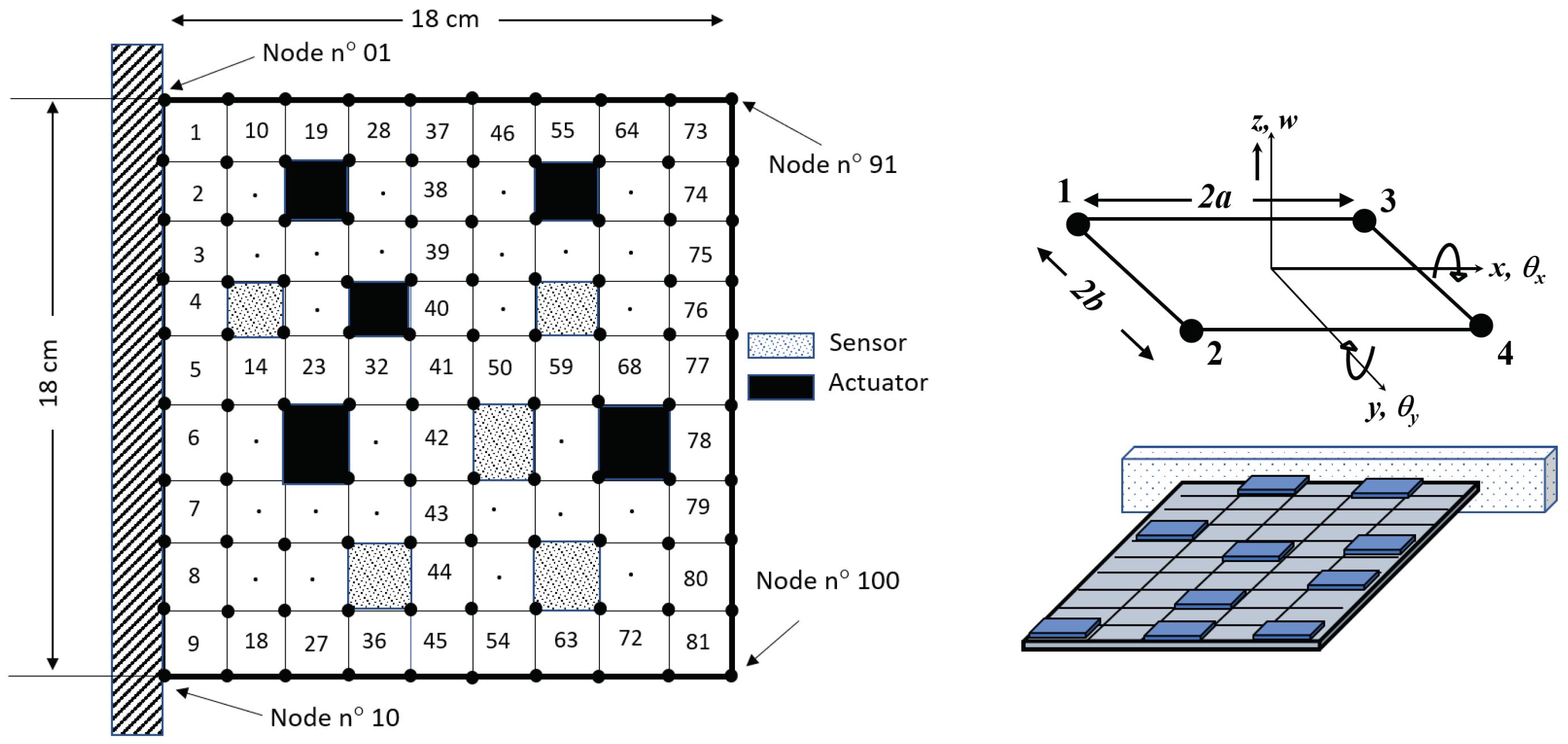
3. Finite Element Formulation

3.1. Full Order Process

In this section, the host plate and the piezoelectric elements are modeled by proceeding to a full-order FE method. Using a finite element with four nodes and Kirchhoff’s classical plate theory, the strains developing in the plate can be written as

$${\left\{\epsilon \right\}}_{3\times 1}=z{\left[{\beta }_u\right]}_{3\times 12}{\left\{u_e\right\}}_{12\times 1}.$$

(13)

where

$${\left[{\beta }_u\right]}_{3\times 12}={\left\{\begin{array}{ccc}-z{\displaystyle \frac{{\partial }^2}{\partial x^2}}& -z{\displaystyle \frac{{\partial }^2}{\partial y^2}}& -2z{\displaystyle \frac{{\partial }^2}{\partial x\partial y}}\end{array}\right\}}_{3\times 1}^T\times {\left[N\right]}_{1\times 12}.$$

(14)

in which ${\left[N\right]}_{1\times 12}$ is the interpolation function and $u_e$ is the element displacement vector. Since the control patches are made using the piezoelectric material PZT-5H for the actuators and PVDF for the sensors, and assuming that the piezoelectric patches are poled in the z-direction, the electric field can be written as

$${\left\{E\right\}}_{3\times 1}=-\left\{{\beta }_{\varphi }\right\}V=-{\left[\begin{array}{ccc}0& 0& 1/h_p\end{array}\right]}^{T}V.$$

(15)

Applying Hamilton’s variational principle, the dynamic equation of one selected finite element of a structure (plate-piezoelectric patches) is given by

$$\left[M_e\right]\left\{{\ddot{u}}_e\right\}+\left[K_e\right]\left\{u_e\right\}=\left\{F_e\right\}.$$

(16)

where $\left[M_e\right]$ and $\left[K_e\right]$ are the elemental mass and stiffness matrices. The total force vector $\left\{Fe\right\}$ acting on the finite element is

$$\left[F^e\right]=F_S^e+F_{T,S}^e+F_{{}_{T,P}}^{{}^e}+F_{E,P}^e.$$

(17)

where the mechanical, the plate material thermal expansion, the piezoelectric material thermal expansion and the electric forces, respectively, are expressed by

$$\begin{array}{ccc}\hfill \left\{F_S^e\right\}& =& {\int }_{A_S}{\left[N\right]}^T\left\{f_S^e\right\}d{A}_S,\hfill \end{array}$$

(18)

$$\begin{array}{ccc}\hfill \{F_{T,S}^e\}& =& 1/2{\int }_{S}z{\left[{\beta }_u\right]}^T\left[C_S\right]\left\{{\alpha }_{{}_S}\right\}\Delta Td\tau ,\hfill \end{array}$$

(19)

$$\begin{array}{ccc}\hfill \{F_{T,P}^e\}& =& 1/2{\int }_{P}z{\left[{\beta }_u\right]}^T\left[C_P\right]\left\{{\alpha }_P\right\}\Delta Td\tau ,\hfill \end{array}$$

(20)

$$\begin{array}{ccc}\hfill \{F_{E,P}^e\}& =& -([K_{u\varphi }^e]+[{\tilde{K}}_{u\varphi }^e])Z_s^{-1}(Q_{ext}^e+Q_{pyr}^e).\hfill \end{array}$$

(21)

where

$$\begin{array}{cc}\hfill [K_{u\varphi }^e]=[K_{\varphi u}^e]& ={\int }_{P}z\left\{{\beta }_u\right\}\left[e^T\right]\left[{\beta }_{\varphi }\right]d\tau ,\hfill \end{array}$$

(22)

$$\begin{array}{cc}\hfill [{\tilde{K}}_{u\varphi }^e]=[{\tilde{K}}_{\varphi u}^e]& ={\int }_{P}z\left\{{\beta }_u\right\}\left[\tilde{e}\right]\left[{\beta }_{\varphi }\right]\Delta Td\tau .\hfill \end{array}$$

(23)

here, $[K_{u\varphi }^e]$ is the electromechanical interaction matrix and $[{\tilde{K}}_{u\varphi }^e]$ is the change in the electromechanical interaction matrix at the applied temperature. The external charge applied on the piezoelectric surface $Q_{ext}^e$, the produced charge on the piezoelectric patch due to the pyroelectric effect $Q_{pyr}^e$ and the sensor capacitance at a reference temperature $Z_s$, are given by

$$\begin{array}{cc}\hfill Q_{ext}^e& ={\int }_{A_P}qd{A}_P,\hfill \end{array}$$

(24)

$$\begin{array}{cc}\hfill Q_{pyr}^e& =\frac{1}{2}{\int }_P{\left\{P\right\}}^T\left\{{\beta }_{{}_{\varphi }}\right\}\Delta Td\tau ,\hfill \end{array}$$

(25)

$$\begin{array}{cc}\hfill Z_s& =([K_{\varphi \varphi }^e]+[{\tilde{K}}_{\varphi \varphi }^e]).\hfill \end{array}$$

(26)

where $[K_{\varphi \varphi }^e]$ is the capacitance of the piezoelectric patches at the reference temperature and $[{\tilde{K}}_{\varphi \varphi }^e]$ is the temporal relative change in this capacitance at a given temperature:

$$\begin{array}{cc}\hfill [K_{\varphi \varphi }^e]& ={\int }_P{\left\{{\beta }_{\varphi }\right\}}^T\left[{\epsilon }^T\right]\left\{{\beta }_{\varphi }\right\}d\tau ,\hfill \end{array}$$

(27)

$$\begin{array}{cc}\hfill [{\tilde{K}}_{\varphi \varphi }^e]& ={\int }_P{\left\{{\beta }_{\varphi }\right\}}^T\left[\tilde{\epsilon }\right]\left\{B_{\varphi }\right\}\Delta Td\tau .\hfill \end{array}$$

(28)

The electrical forces on a piezoelectric patch are due to the thermal strain effect, the pyroelectric effect, and external charges. The voltage produced across these patches can be written as

$$\begin{array}{c}V={\left([K_{\varphi \varphi }^e]+[{\tilde{K}}_{\varphi \varphi }^e]\right)}^{-1}\left\{Q_{ext}^e+Q_{pyr}^e+\left([K_{\varphi u}^e]+[{\tilde{K}}_{\varphi u}^e]\right)\left\{u_e\right\}\right\}\end{array}.$$

(29)

3.2. Modal Analysis

Using uncoupled equations, the analysis of the coupled equations System (16) becomes easier and the multi-degree freedom system can be replaced by a single-degree freedom system using modal analysis. The process consists in adopting the following transformation

$${\left\{X\right\}}_{n\times 1}={\left[H\right]}_{n\times r}{\left\{\eta \right\}}_{r\times 1}.$$

(30)

where $\left[H\right]$ is the eigen-vector matrix, $\left\{\eta \right\}$ is the modal displacement vector, n is the total number of dofs of the structure and r is the considered number of modes. Assuming a linear damping as a combination of the mass and stiffness matrices, the uncoupled dynamic equations can be rewritten as

$${\ddot{\eta }}_m+c_m\dot{\eta }+{\omega }_m^2{\eta }_m=f_m.$$

(31)

where $c_m=2{\zeta }_m{\omega }_m=\mu +\lambda {\omega }_m^2$ with the given modal damping ratio ${\zeta }_m=\frac{\mu }{2{\omega }_m}+\frac{\lambda {\omega }_m}{2}$. Here, “m” denote a mode number and the ($\mu$,$\lambda$) correspond to the mass and stiffness proportional Rayleigh damping coefficients.

The uncoupled Equation (31) represents the equation of motion of the $m_{th}$ mode of a smart plate. The three first five modal frequencies are calculated at a reference temperature using commercial software for the derived FEM model. Applying the boundary conditions of the plate with one cantilevered edge, the Equation (17) can be transformed as

$${\left\{F\right\}}_{270\times 1}={\left\{F_S\right\}}_{270\times 1}+{\left\{F_{T,S}\right\}}_{270\times 1}+{\left\{F_{T,P}\right\}}_{270\times 1}+{\left\{F_{E,P}\right\}}_{270\times 1}.$$

(32)

Assuming that the external surface force $F_S=0$ and the thermal expansion force $F_{TS}=0$, the modal force vector $\left\{f\right\}={\left[H\right]}^T\left\{F\right\}$, depending on the pyroelectric effect, can be evaluated. Substituting $\left\{F_{T,P}\right\}=F_{pth}$ and the value of $\left\{F_{E,P}\right\}$ from Equation (17) into Equation (32), we can obtain the following modal force

$$\left\{f\right\}={\left[H\right]}^T\left\{F_{{}_{pth}}-\left([K_{u\varphi }^e]+[{\tilde{K}}_{u\varphi }^e]\right)Z_s^{-1}(Q_{{}_{ext}}+Q_{{}_{pyr}})\right\}.$$

(33)

where $Q_{ext}=Z_{act}{V}_{ext}$ is the total external charge applied on the actuator surface. The component of the modal force $\left\{f\right\}$ which depends upon the applied external voltage ($V_{ext}$) on the actuator is known as the ‘modal control force’ and is given by

$$\left\{f_c\right\}=-{\left[H\right]}^T\left([K_{u\varphi }^e]+[{\tilde{K}}_{u\varphi }^e]\right)Z_s^{-1}{Z}_{act}{V}_{ext}.$$

(34)

when sensor and actuator patches are subjected to the same temperature, we have $Z_s=Z_{act}$, and the modal control force becomes

$$\begin{array}{c}\left\{f_c\right\}=-{\left[H\right]}^T\left([K_{u\varphi }^e]+[{\tilde{K}}_{u\varphi }^e]\right)Z_s^{-1}{Z}_{act}{V}_{ext}=-{\left[H\right]}^T\left([K_{u\varphi }^e]+[{\tilde{K}}_{u\varphi }^e]\right)V_{ext}\end{array}.$$

(35)

3.3. General Reduction Model

The reduced-order modeling is a global reduction process based on the eigenvalue analysis of the FEM model. There are two reduction process levels; the modal reduction and the dofs reduction. The transformation matrix obtained using this process transforms the full model to a short model using selected eigen-modes with some arbitrary dofs.

Consider an equivalent Kirchhoff plate model element of the above section with four nodes, two mechanical dofs ($\omega ,\theta$), one electric dof ($\varphi$) and one temperature dof ($\theta$) at each node (Figure 1). The FEM model of the plate is derived using Hamilton’s principle; the compact equation of motion for an undamped system with electromechanical coupling can be rewritten as

$$\begin{array}{c}\hfill M_{qq}\ddot{q}+K_{qq}q+K_{q\varphi }\varphi -F=0\end{array}$$

(36)

$$\begin{array}{c}\hfill K_{\varphi q}q+K_{\varphi \varphi }\varphi -Q_a=0\end{array}$$

(37)

where $K_{q\varphi }$, $K_{\varphi \varphi }$, $\varphi$ and $Q_a$ are the electromechanical stiffness matrix, the stiffness matrix due to electrical dofs, the piezoelectric actuator’s electrical vector, and the vector of the electrical charge, respectively.

Substituting $\varphi$ from Equation (37) into Equation (36), the dynamic equation in damped and compact form is given by

$$M\ddot{X}\left(t\right)+C\dot{X}\left(t\right)+KX\left(t\right)=F\left(t\right).$$

(38)

where M, C, and K are, respectively, the mass, damping, and stiffness matrices of the full-order model. $X\left(t\right)$, $\dot{X}\left(t\right)$ and $\ddot{X}\left(t\right)$ represent the displacement, velocity and acceleration vectors. To apply the reduced-order model, Equation (38) will be used in the next formulation. Using a modal matrix, the system can be written in terms of modal coordinates and for “j” eigen-modes as

$$X\left(t\right)={\psi }_{(n\times j)}{\widehat{q}}_{(j\times 1)}\left(t\right).$$

(39)

If only “a” eigen-modes are considered, the solution can be written as

$$X\left(t\right)={\psi }_{(n\times a)}{q}_{(a\times 1)}\left(t\right).$$

(40)

The full-order model can be decomposed into master and slave degrees of freedom. For only “j” selected eigen-modes in Equation (40), we can write in terms of active dofs

$$X\left(t\right)=\left\{\begin{array}{c}{X}^{{}^m}\left(t\right)\\ X^{{}^s}\left(t\right)\end{array}\right\}\approx \left\{\begin{array}{c}{\psi }^{{}^m}\left(t\right)\\ {\psi }^{{}^s}\left(t\right)\end{array}\right\}.{\widehat{q}}_j\left(t\right).$$

(41)

where ${\widehat{q}}_j$ is the modal matrix having “j” modes, and “m” and “s” denote the superscripts corresponding to the master and slave dofs. Moreover, here, ${\psi }^{{}^m}ϵ{\Re }^{{}^{m\times j}}$ and ${\psi }^sϵ{\Re }^{{(}^{n-m)\times j}}$. Considering only the master dofs, the responses in modal form can be given as

$${\widehat{q}}_j\left(t\right)={\psi }_{{}_T}^{{}^m}{X}^{{}^m}\left(t\right).$$

(42)

Since the matrix ${\psi }_{{}_T}^{{}^m}$ may not be a square, the number of modes and number of dofs in the analysis may be the same—this depends on the problem and hence the matrix. The different selection possibilities of modes and dofs are cited in [25]. Substituting Equation (42) in Equation (41), the modal vector can be written as

$$X\left(t\right)=\psi {\psi }_{{}_T}^{{}^m}{X}^{{}^m}\left(t\right)=T_{{}_r}{X}^{{}^m}.$$

(43)

where $\left(T_r\right)$ is the transformation matrix that transforms the full-order model into a reduced-order model. Using this transformation matrix, the full-order model matrices in reduced dimensions can be written as

$$M_{{}_r}=T_r^{{}^T}M{T}_{{}_r};K_r=T_{{}_r}^{{}^T}K{T}_{{}_r};C_r=T_{{}_r}^{{}^T}C{T}_{{}_r}.$$

(44)

here, $M_{{}_r},K_{{}_r}$, $C_{{}_r}$ and $F_{{}_r}\left(t\right)=T_{{}_r}^{{}^T}F\left(t\right)$ represent the mass, stiffness, damping matrices, and force vector expressed in the reduced-order model, respectively. The selection of modes and dofs are governed by the type of system and the conditions of the external charges.

3.4. Monte Carlo Method

A Monte Carlo method is used here to randomly select the number of sensors and their discrete locations along the plate. This selection is established by minimizing the variance and depends on a random points choice of the degrees of freedom of the sensor locations. Applying this distribution, the measurements are randomly allocated by the selected points. MCS requires the specification of dimensions, the FEM grid map, the density of nodes for each region in the plate and, finally, the computational number of samples of repetition $n_{mc}$. For each point in the grid, the generation of the grid map, depending on prefixed dimensions and data, is randomly established from the defined statistical properties of the studied model. The selected random points are chosen from the grid map and the spatial analysis procedure is performed as a function of the different values of location. The optimized variables are determined from the mean-variance values and stored. The above steps are repeated until the minimal mean-variance is found. Therefore, the sensor locations that generated the minimum mean-variance are the most optimal sensor placements based on these repetitions.

4. Control Design

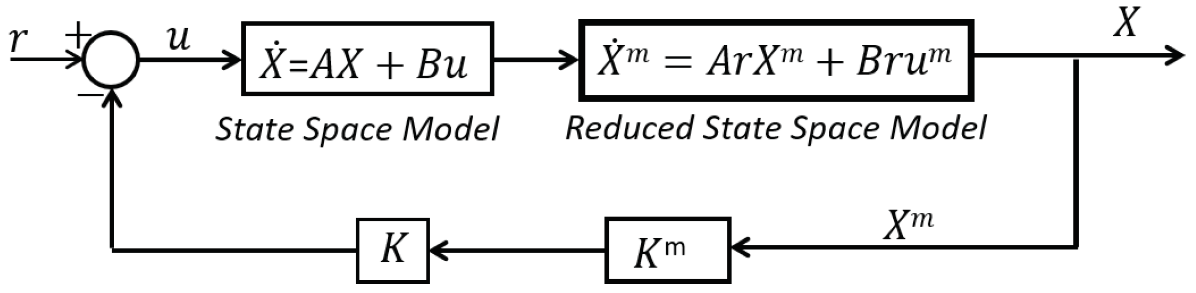
4.1. State Space Model

To control the response of a composite plate using an active vibration control procedure, the uncoupled equations of motion have to be converted into a state-space (SS) model. Therefore, in this section, the uncoupled equations are rewritten in an SS form to represent the structure in a first differential order. The state variables of the structure, hence, are given by

$$\left\{\dot{s}\right\}=\left[A\right]\left\{s\right\}+\left[B\right]u.$$

(45)

where $\left(\dot{s}\right)$ is the first time derivative of the state variables and u is the input of the control box. The sensor outputs are a function of $\left\{s\right\}$ and are given by

$$\left\{y\right\}=C\left\{s\right\}.$$

(46)

Converting the first three modal equations of motion into the state space form by ${\dot{\eta }}_{(j=1,2,3)}=x_{(j=1,2,3)}$ and using Equation (31), the first three modes can be given by

$${\dot{x}}_j+c_j{x}_j+{\omega }_j^{{}^2}{\eta }_j=f_j,(j=1,2,3).$$

(47)

or in matrix form

$$\left(\begin{array}{cccccc}0& 0& 0& 1& 0& 0\\ 0& 0& 0& 0& 1& 0\\ 1& 0& 0& 0& 0& 1\\ 1& 0& 0& 0& 0& 0\\ 0& 1& 0& 0& 0& 0\\ 0& 0& 1& 0& 0& 0\end{array}\right)\left\{\begin{array}{c}{\dot{\eta }}_1\\ {\dot{\eta }}_2\\ {\dot{\eta }}_3\\ {\dot{x}}_1\\ {\dot{x}}_2\\ {\dot{x}}_3\end{array}\right\}+\left(\begin{array}{cccccc}{\omega }_1^2& 0& 0& c_1& 0& 0\\ 0& {\omega }_2^2& 0& 0& c_2& 0\\ 0& 0& {\omega }_3^2& 0& 0& c_3\\ 1& 0& 0& -1& 0& 0\\ 0& 1& 0& 0& -1& 0\\ 0& 0& 1& 0& 0& -1\end{array}\right)\left\{\begin{array}{c}{\eta }_1\\ {\eta }_2\\ {\eta }_3\\ x_1\\ x_2\\ x_3\end{array}\right\}=\left\{\begin{array}{c}{f}_1\\ f_2\\ f_3\\ 0\\ 0\\ 0\end{array}\right\}.$$

(48)

where

$$\left[\begin{array}{ccc}1& 0& 0\\ 0& 1& 0\\ 0& 0& 1\end{array}\right]={\left[H\right]}^{{}^T}\left[M\right]\left[H\right],\left[\begin{array}{ccc}{c}_1& 0& 0\\ 0& c_2& 0\\ 0& 0& c_3\end{array}\right]={\left[H\right]}^{{}^T}\left[C\right]\left[H\right],\left[\begin{array}{ccc}{\omega }_1^2& 0& 0\\ 0& {\omega }_2^2& 0\\ 0& 0& {\omega }_3^2\end{array}\right]={\left[H\right]}^{{}^T}\left[K\right]\left[H\right].$$

(49)

are the modal mass, modal damping, and modal stiffness sub-matrices, respectively. $\left[H\right]$ is the normalized eigenvector matrix. (45) can be rewritten as

$$\left\{\dot{s}\right\}=\left[A\right]\left\{s\right\}+\left[B\right]V_{{}_{ext}}+\left[G\right].$$

(50)

with $\left\{s\right\}={\left\{{\eta }_1{\eta }_2{\eta }_3{x}_1{x}_2{x}_3\right\}}^T$ and $\left[G\right]$ is the matrix corresponding to the thermal strain and to the pyroelectric effects. Equation (50) is the state space model equation. From Equation (29), the voltage produced by the sensors due to deformations of the plate is given by

$$V_{{}_{sens}}=Z_{{}_{sens}}^{{}^{-1}}(Q_{{}_{pyr}}+([K_{{}_{u\varphi }}^{{}^e}]+[{\tilde{K}}_{{}_{u\varphi }}^{{}^e}])u_{{}_e}).$$

(51)

4.2. LQR Control

A linear quadratic regulator (LQR) controller was used and implemented here for comparison with the LQG-Kalman scheme. Therefore, the SS is converted to the reduced-order state model, as shown in Figure 2. The actuator inputs are obtained through the LQR algorithm by minimizing the cost function $(J)$ defined by

$$J=\underset{\tau \to \infty }{lim}\frac{1}{\tau }\left[{\int }_0^{\infty }\left\{{(X^m)}^{T}Q(X^m)+{(u^m)}^{T}R(u^m)\right\}dt\right].$$

(52)

where Q and R are the weight matrices of the state space variable $X^m$ and the input $u^m$. By minimization of the quadratic cost function defined in Equation (52) and using the dynamic equation, we obtain the state feedback in the form of the required control input $u^m$ as follows

$$u^m=-K_s{X}^m.$$

(53)

where $K_s$ is the $(m\times r)$ gain matrix resulting from the reduced model. The gain of a closed loop is determined by solving the Riccati reduced-matrix. With this gain matrix, the control input needed to control the full-order model dynamics of the plate can, hence, be estimated. The capacitance of sensor patch $Z_s$ can be evaluated at an initial temperature by

$$\begin{array}{ccc}\hfill Z_s={\breve{K}}_{\varphi \varphi }^e& =& ([K_{\varphi \varphi }^e]+[{\tilde{K}}_{\varphi \varphi }^e]).\hfill \end{array}$$

(54)

where $[K_{\varphi \varphi }^e]$ is the capacitance of a piezoelectric patch at reference temperature and $[{\tilde{K}}_{\varphi \varphi }^e]$ are the changes in the capacitance at a given temperature. For an initial temperature, the voltage generated across a piezoelectric patch and a modal force at reference temperature can be written as

$$\begin{array}{c}\hfill V={[K_{\varphi \varphi }^e]}^{-1}\left[Q_{ext}^e+[K_{\varphi \varphi }^e]\left\{u_e\right\}\right],\end{array}$$

(55)

$$\begin{array}{c}\hfill \left\{F_c\right\}={[H]}^T\left([K_{u\varphi }^e]{[K_{\varphi \varphi }^e]}^{-1}{Q}_{ext}\right).\end{array}$$

(56)

Using identical sensor and actuator patches at the same temperature, the modal control force becomes

$$\left\{F_c\right\}=-{\left[H\right]}^T[K_{u\varphi }^e]V_{ex}.$$

(57)

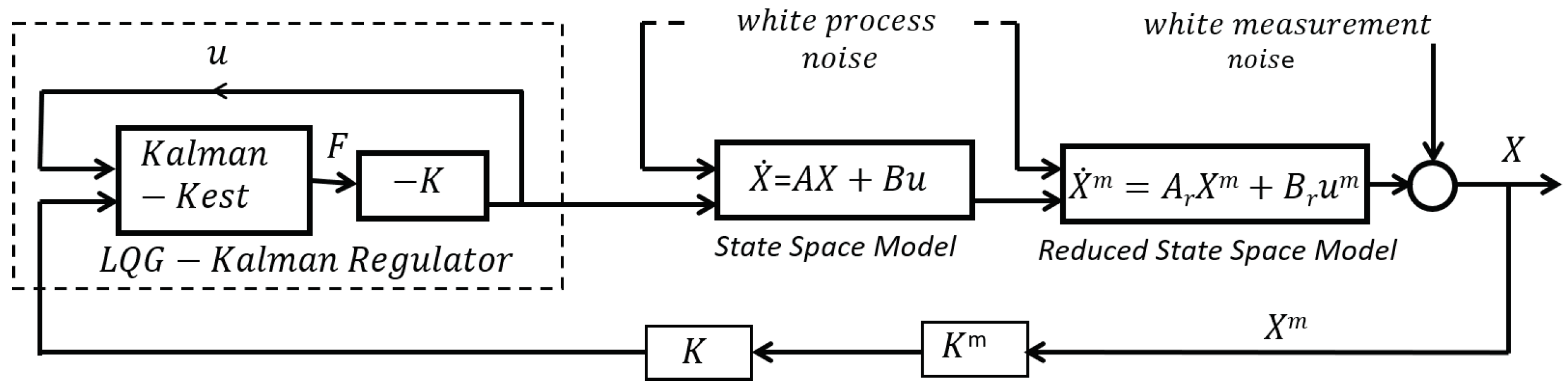
4.3. LQG-Kalman Estimator

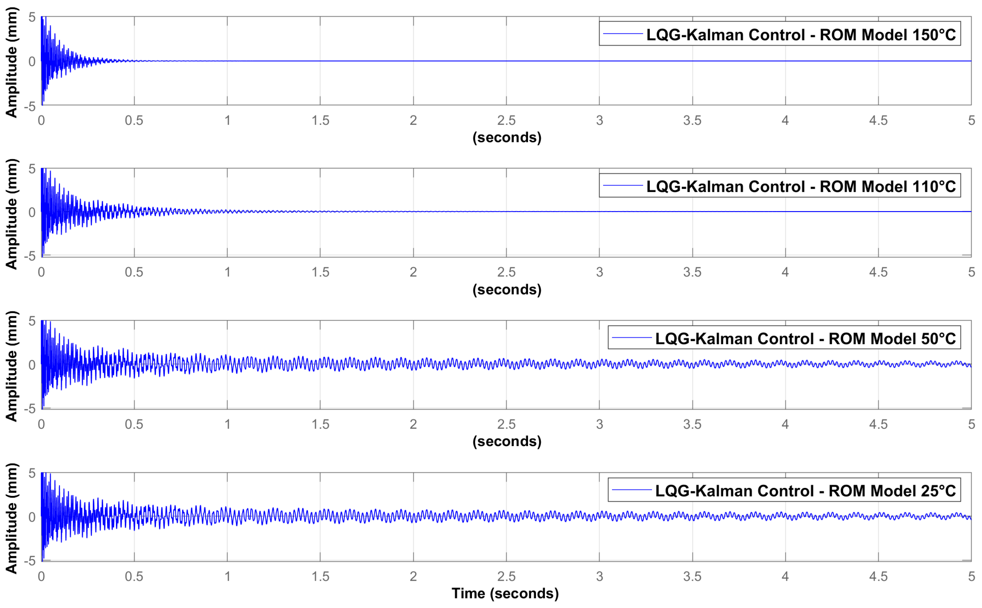
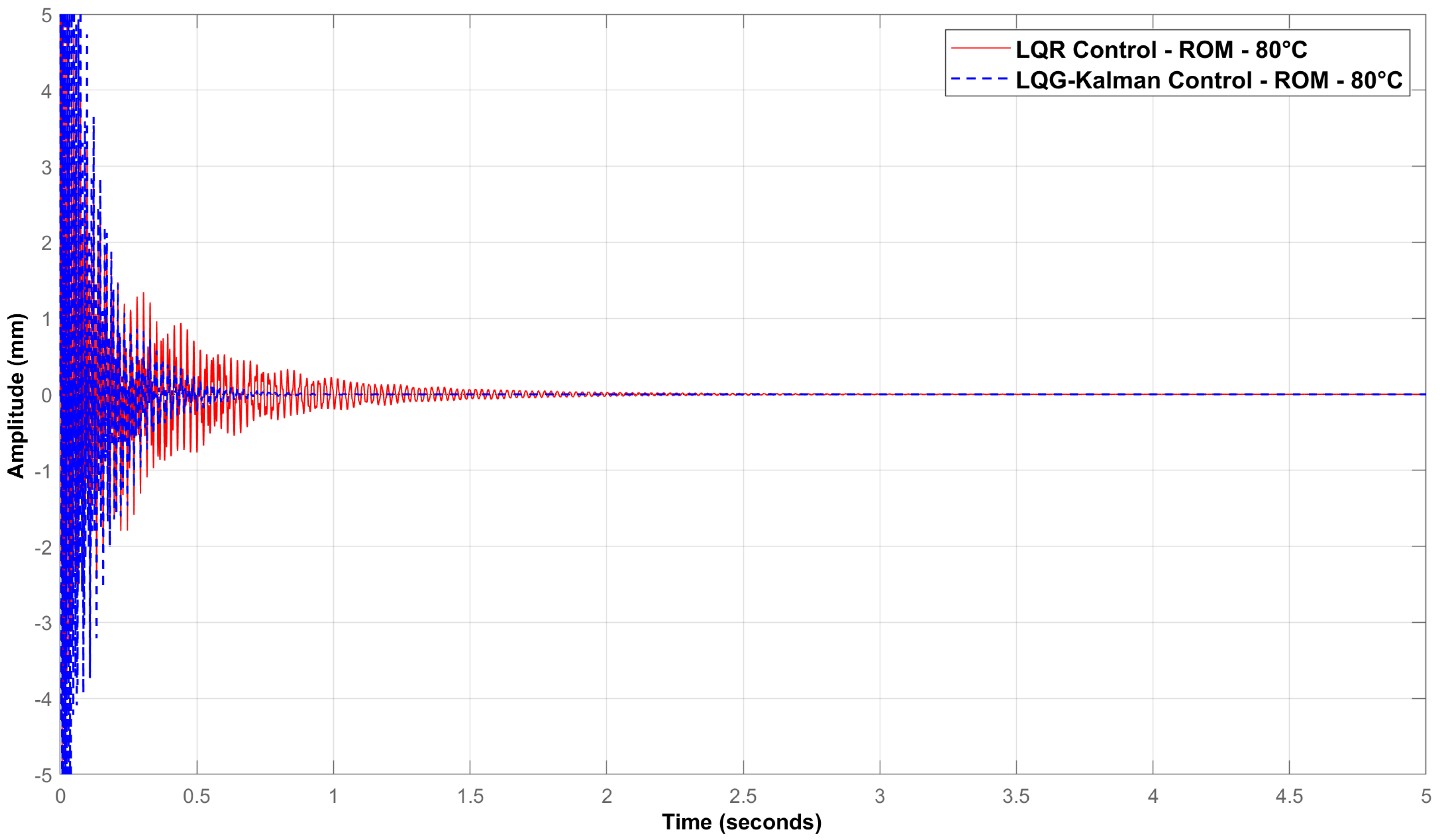
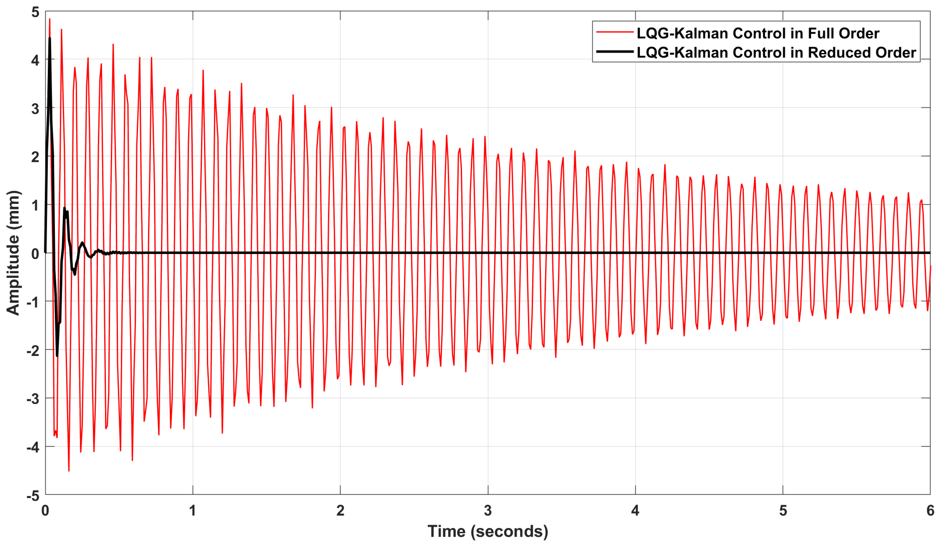
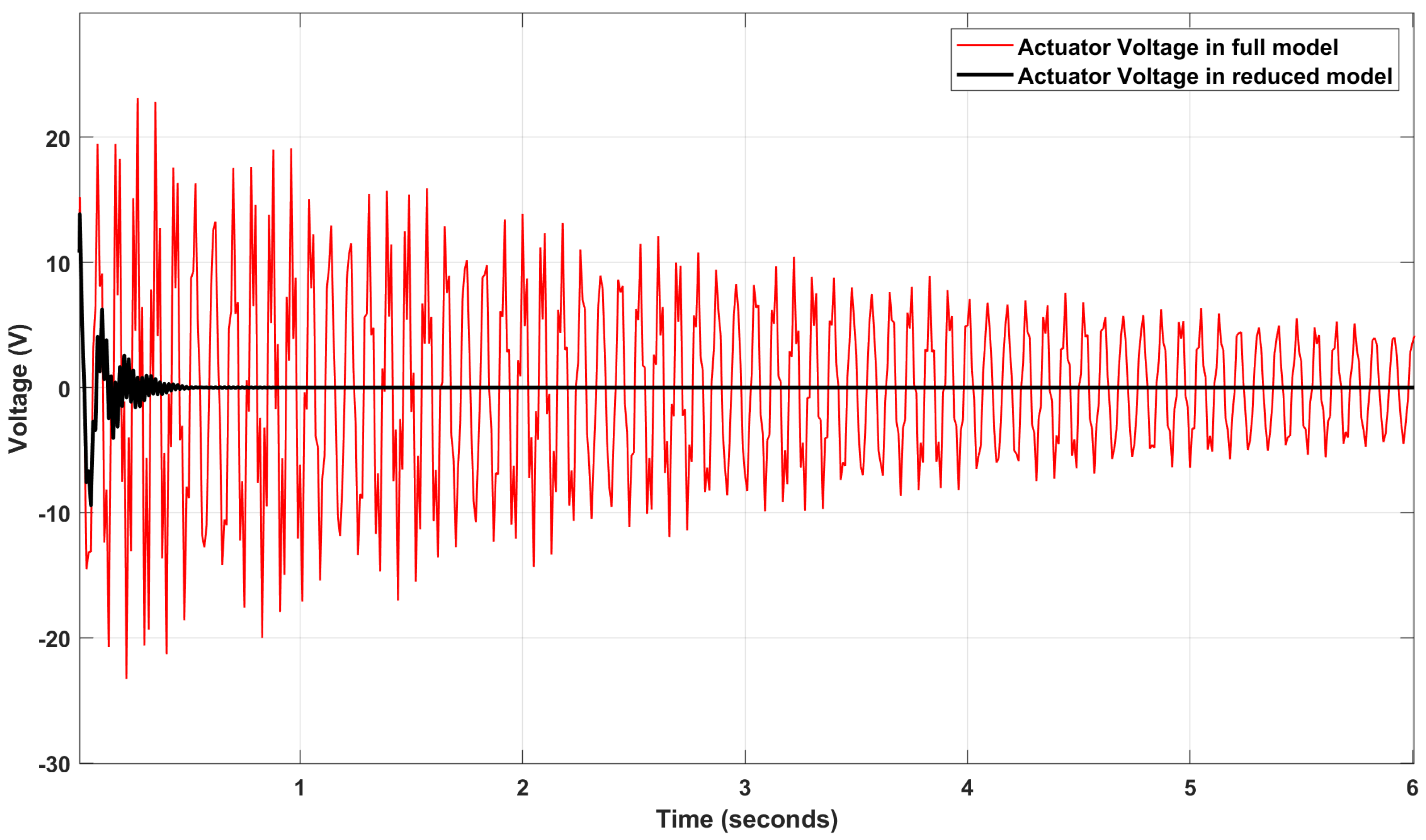
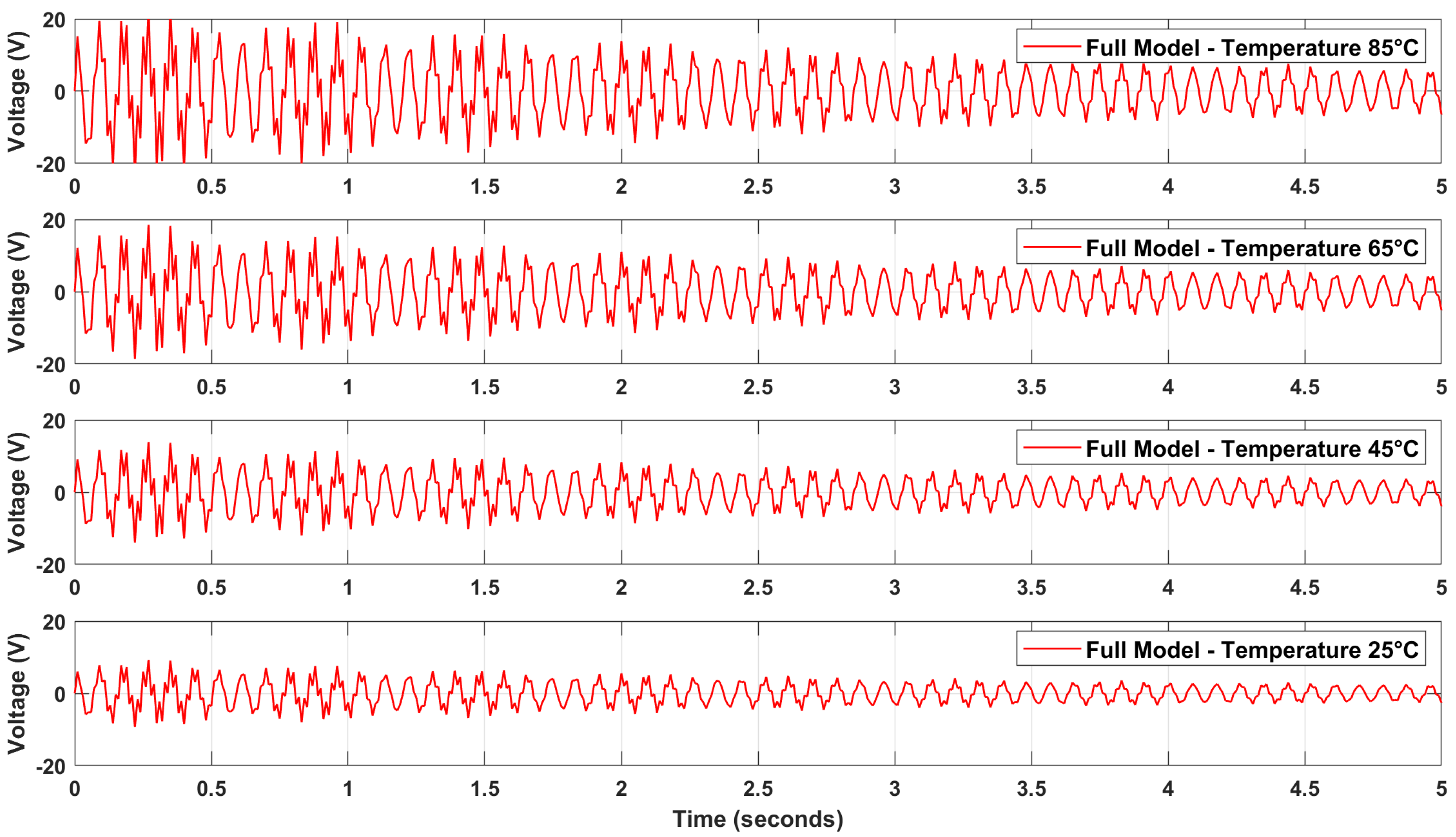
The filter of Kalman is a computational estimator based on two cycles: time and measurement updates. It is used to identify the mechanical displacements and the parameters of a system. Its advantage is that the dynamic noise can be included in the dynamical state model. It is a real time estimator supplying the estimates for an available measurement at a given instant. The filter algorithm is generally a set of analytical equations that implement a prediction (correction-estimation) that is optimal in the sense of minimizing the estimated error covariance in some control conditions. For a studied plate, the feedback control system (LQG-Kalman filter) requires the measurement of tip deflection and its rate. By adding the filter of Kalman, the control design gives the required potential noise control. For this purpose, in the proposed scheme in Figure 3, the noise has been introduced as an auxiliary gain to be highly sensible to noise. In addition, sometimes, due to the nature of the system input to the non-linearity or modal frequency, the system response becomes unstable. This can be solved by filtering the output response in the controller feedback (using measurement data). According to [26,27], the system can be represented as a linear stochastic difference relation as

$$\left\{\dot{x}\right\}=[A]\left\{x\right\}+[B]u+w.$$

(58)

Using the state equation of the structure (50), a first modal control force, a control voltage and a voltage in the sensor are given by

$$\begin{array}{ccc}\hfill \left\{F_c\right\}& =& -{[H]}^T[K_{u\varphi }^e]\left\{V_{ex}\right\},\hfill \end{array}$$

(59)

$$\begin{array}{ccc}\hfill V_{ext}& =& {\left({[H]}^T[K_{u\varphi }^e]\right)}^{-1}k{\dot{\eta }}_e,\hfill \end{array}$$

(60)

$$\begin{array}{ccc}\hfill V_{sens}& =& {[K_{\varphi \varphi }^e]}^{-1}\left[[K_{u\varphi }^e]\left\{u_e\right\}\right].\hfill \end{array}$$

(61)

where ${\dot{\eta }}_e$ is estimated using the Kalman observer. The modal displacements and velocities are estimated using the Kalman observer/estimator and can be constructed as

$$\begin{array}{ccc}\hfill \left\{{\dot{\eta }}_e\right\}=& [A_d]\left\{{\eta }_e\right\}+[B_d]V_{ext}+[L]\left(V_{sens}-[X]\left\{{\eta }_e\right\}\right),\hfill & \\ \hfill \left\{{\dot{\eta }}_e\right\}=& \left\{{\eta }_e\right\}+[M](V_{sens}-[X]\left\{{\eta }_e\right\}).\hfill \end{array}.$$

(62)

where ${\eta }_e$ is the estimated vector in full state and $[A_d]$, $[B_d]$ are discretized forms of $[A]$ and $[B]$. $[L]$ and $[M]$ are the Kalman filter gain matrices. $V_{sen}$ is the sensor voltage and X is the sensor location vector. The matrices $[B],[X],[L]$ and $[M]$ and the state vector ${\dot{\eta }}_e$ all depend on the electromechanical and permittivity coefficients of the used piezoelectric material. The external control voltage to be applied to the actuator patch and corresponding to the modal control force is given by [28]

$$V_{ctrl}=-\frac{G{\dot{\eta }}_e}{{[H]}^T{Z}_{act}}.$$

(63)

where g is the velocity gain of the controller, H is the modal matrix of the first three modes, $Z_{act}$ is the capacitance of the actuator and $f_c$ is the corresponding control force.

5. Discussion

This paper presents an analysis of the behavior of a smart piezocomposite plate, actively controlled in a reduced model and under different values of temperature. Two types of controllers are used: a robust LQG-Kalman controller and an optimal LQR controller. The Kalman filter is based on an analytical model deduced from FEM formulation and the LQR is a regulator based on velocity feedback of the first modal state.

To perform this comparison, to verify the robustness of the LQG-Kalman control, and to analyze the effects of temperature changes and the distribution of sensors, a thin one-side cantilevered square plate of 18 cm × 18 cm × 0.08 cm size is considered, as shown in Figure 1. A range of piezoelectric actuators (PZT) and sensors (PVDF) are randomly distributed along the plate. They are assumed to be perfectly symmetrically bonded upon the top and the bottom sides of the plate. The material properties of both the piezoelectric elements and the host plate are presented in

Table 1. Material properties of the piezoelectric elements and the host plate.

Properties	Actuators PZT	Sensors PVDF	Host Plate
Length (cm)	$l_a$	$l_s$	18
Width (cm)	$b_a$	$b_s$	18
Thickness (cm)	$0,6$	$0,5$	$0,08$
Piezoelectric constant (pm/V) $d_{31},d_{32},d_{33},d_{24},d_{15}$	−220, −220, 374, 670, 670	−22, 22, 0, 0, 0	—
Permittivity (nF/m) ${ϵ}_{11}={ϵ}_{22}\approx {ϵ}_{33}$	15, 3	0, 1062	—
Density (Kg/m${}^3$)	7600	2700	1800
Young’s modulus E (GPa)	63	$2.0$	70

. The plate is divided into 81 quadrilateral finite elements of the same size. The plate element is modeled using Kirchhoff’s theory and has four nodes (Figure 1). Each node has three mechanical dofs (one translation and two rotations), one electrical dof, and one thermal dof.

To establish the control procedure, the sensors are distributed over the entire surface of the plate and in three areas. The first area is near the cantilever edge (element numbers 1 to 27); the second area corresponds to the middle of the plate (elements 28 to 54); and the third concerns the end-edge of the plate (elements 55 to 81). For each distribution, the MCS method is used to select the dofs of elements having the maximum electrical responses, i.e., those which correspond to the significant mechanical deformations (including deformation due to temperature increase, i.e., the pyroelectric effect), which allows the actuator to act locally and not over the entire surface of the plate. The comparison of the control response is, then, accomplished between all proposed distributions. The numeric formulation and control implementation of the structure is achieved using commercial software.

The first vibration mode shapes of the plate are visualized. Impulse responses at the end of the plate are traced. The sensor voltage output, the control voltage applied to the actuator input, the total control deformations, and the state vector estimated by the Kalman observer at different temperatures are evaluated and simulated. The control is next compared to the LQR algorithm to evaluate of his efficiency. Figure 4 and Figure 5 present the first 3D mode shapes of vibration with relative frequencies of the one-edge-cantilevered plate. Figure 6 shows deformation responses using LQG-Kalman control in full and reduced order models for an ambient temperature $25{}^{°}$C. The MCS is applied here to select 20 active dofs from the distributed sensors and with 100 computational number of repetition samples. The Figure 7 compare, in the reduced order model, the impulse response of the strategies of control (LQR and LQG-Kalman) at a temperature $80{}^{°}$C with the same situation of MCS distribution and sensor positions. The comparison between full and reduced order model using LQG-Kalman procedure has been established in Figure 8. the actuator input voltages are given in Figure 9 in both full and reduced models.

Figure 10 and Figure 11 illustrate, in the reduced and full models, the sensor outputs for multiple temperatures: (25 ${}^{°}$C, 45 ${}^{°}$C, 65 ${}^{°}$C, and 85 ${}^{°}$C). Figure 12 shows a comparison of the responses of the control according to the selection of the nodes and which belong to the sensors distributed on the three parts of the plate (the embedded, middle, and free parts). It is noted that it is preferable to multiply the number of sensors to ensure a very good selection through the MCS and to obtain the maximum amount of information on all parts of the plate undergoing the deformations. These are not filtered and contribute to forming the output of all the sensors, which are then introduced into the control box, processed and transmitted to the actuators, which act on their part on the plate.

6. Conclusions

In this study, the active vibration control and thermal effects of a piezo-composite plate are analyzed. Representations of the two procedures of control, i.e., LQR and LQG-Kalman, are established in a reduced model and performed. Based on the problem formulation, the control performance depends on the sensor voltage output, the actuator control voltage (proportional to the control effort), the Kalman filter algorithm and changes in temperature. Further, to maintain the control performance for all temperatures and noise perturbations, the Kalman observer is generally added to the LQG regulator. Therefore, it is concluded that the control is more effective using the reduced model formulation compared to the full model. The simulations demonstrated the robustness of the control law with respect to temperature variations and unpredictable perturbations. The quality of control can be improved by choosing adequate controls to be used as a function of the nature of the perturbations of the structures. The control voltage applied to the inputs of the actuators depends on the number of modes to be controlled, the type of control law, and the piezoelectric material of the actuators. The selection of active dofs produced by the MCS distribution helps in the selection of the nodes with high amplitude of mechanical displacement and neglects the dofs with low amplitudes. All displacements having a low amplitude are ignored under some criteria. The simulations, relative to the reduced model, also show the feasibility, and the effectiveness, of the LQG-Kalman control under thermal conditions.

References

1. Tauchert, T. Piezotheelmoelastic behavior of a laminated plate. J. Therm. Stress. 1992, 15, 25–37. [Google Scholar] [CrossRef]
2. Lee, H.; Saravanos, D. Generalized finite element formulation for smart multilayered thermal piezoelectric composite plates. Int. J. Solids Struct. 1997, 34, 3355–3371. [Google Scholar] [CrossRef]
3. Caruso, G.; Galeani, S.; Menini, L. Active vibration control of an elastic plate using multiple piezoelectric sensors and actuators. Simul. Model. Pract. Theory 2003, 11, 403–419. [Google Scholar] [CrossRef]
4. Kumar, K.; Narayanan, S. The optimal location of piezoelectric actuators and sensors for vibration control of plates. Smart Mater. Struct. 2007, 16, 2680–2691. [Google Scholar] [CrossRef]
5. Dong, X.; Meng, G.; Peng, J. Vibration control of piezoelectric smart structures based on system identification technique: Numerical simulation and experimental study. J. Sound Vib. 2006, 297, 680–693. [Google Scholar] [CrossRef]
6. Xu, S.; Koko, T. Finite element analysis and design of actively controlled piezoelectric smart structure. Finite Elem. Anal. Des. 2004, 40, 241–262. [Google Scholar] [CrossRef]
7. Kim, H.; Sohn, J.; Choi, S. Vibration control of a cylindrical shell structure using macro fibre composite actuators. Mech. Based Des. Struct. Mach. 2011, 39, 491–506. [Google Scholar] [CrossRef]
8. Kusculuoglu, Z.; Royston, T. Finite element formulation for composite plates with piezoceramic layers for optimal vibration control applications. Smart Mater. Struct. 2005, 14, 1139–1153. [Google Scholar] [CrossRef]
9. Tzou, H.; Bao, Y. Nonlinear piezothermoelasticity and multi-field actuations. J. Vib. Acoust. 1997, 119, 374–381. [Google Scholar] [CrossRef]
10. Sanbi, M.; Saadani, R.; Sbai, K.; Rahmoune, M. Thermoelastic and Pyroelectric Couplings Effects on Dynamics and Active Control of Smart Piezolaminated Beam Modeled by Finite Element Method. Smart Mater. Res. 2014, 2014, 145087.1–145087.10. [Google Scholar] [CrossRef]
11. Sanbi, M.; Saadani, R.; Sbai, K.; Rahmoune, M. Thermal Effects on Vibration and Control of Piezocomposite Kirchhoff Plate Modeled by Finite Elements Method. Smart Mater. Res. 2015, 2015, 1–15. [Google Scholar] [CrossRef]
12. Mitchell, J.; Reddy, H. A refined hybrid platetheoryfor composite laminates with piezoelectric laminae. Int. J. Solids Struct. 1995, 32, 2345–2367. [Google Scholar] [CrossRef]
13. Gu, H.; Chattopadhyay, A.; Li, J.; Zhou, X. A higher order temperature theory for coupled thermopiezoelectric-mechanical modeling of smart composites. Int. J. Solids Struct. 2000, 37, 6479–6497. [Google Scholar] [CrossRef]
14. Hughes, P.; Skelton, R. Modal truncation for flexible spacecraft. J. Guid. Control 1981, 4, 291–297. [Google Scholar] [CrossRef]
15. Willcox, K.; Peraire, J. Balanced model reduction via the proper orthogonal decomposition. AIAA J. 2002, 40, 2323–2330. [Google Scholar] [CrossRef]
16. Hsieh, W. Nonlinear principal component analysis by neural networks. Tellus A 2002, 53, 2323–2330. [Google Scholar] [CrossRef]
17. Callahan, J.; Avitabile, P.; Riemer, R. System equivalent reduction expansion process (SEREP). In Proceedings of the 7th International Modal Analysis Conference, Las Vegas, NV, USA, 30 January–2 February 1989; Union College: Schenectady, NY, USA, 1989; pp. 29–37. [Google Scholar]
18. Sharma, M.; Singh, S.; Sachdeva, B. Modal control of a plate using fuzzy logic controller. Smart Mater. Struct. 2007, 16, 1331–1341. [Google Scholar] [CrossRef]
19. Tanaka, N.; Sanada, T. Modal control of a rectangular plate using smart sensors and smart actuators. Smart Mater. Struct. 2007, 16, 36. [Google Scholar] [CrossRef]
20. Rader, A.; Afagh, F.; Yousefi-Koma, A.; Zimcik, D. Optimization of piezoelectric actuator configuration on a flexible fin for vibration control using genetic algorithms. J. Intell. Mater. Syst. Struct. 2007, 18, 1015. [Google Scholar] [CrossRef]
21. Spier, C.; Bruch, J.; Sloss, J.; Adali, S.; Sadek, I. Placement of multiple piezo patch sensors and actuators for a cantilever beam to maximize frequencies and frequency gaps. J. Vib. Control 2009, 15, 643. [Google Scholar] [CrossRef]
22. Sharma, S.; Vig, R.; Kumar, N. Temperature compensation in a smart structure by the application of DC bias on piezoelectric patches. J. Intell. Mater. Struct. 2016, 27, 2524–2535. [Google Scholar] [CrossRef]
23. Gupta, V.; Sharma, M.; Thakur, N. Active structural vibration control: Robust to temperature variations. Mech. Syst. Signal Process. 2012, 33, 80. [Google Scholar] [CrossRef]
24. Nowacki, W. Some general theorems of thermopiezoelectricity. J. Therm. Stress. 1978, 1, 171–182. [Google Scholar] [CrossRef]
25. Lal, H.; Sarkar, S.; Gupta, S. Stochastic model order reduction in randomly parametered linear dynamical systems. Appl. Math. Model. 2017, 51, 744–763. [Google Scholar] [CrossRef]
26. Anderson, B.; Moore, J. Optimal Filtering; Thomas Kailath Editor: Piscataway, NJ, USA, 1979. [Google Scholar]
27. Simon, D.; Curadelli, O.; Ambrosini, D. Kalman Filtering for fuzzy discrete time dynamic systems. Appl. Soft Comput. 2003, 3, 191–207. [Google Scholar] [CrossRef]
28. Garrido, H.; Curadelli, O.; Ambrosini, D. A straightforward method for tuning of Lyapunov based controllers in semi active vibration control applications. J. Sound Vib. 2014, 333, 1119–1131. [Google Scholar] [CrossRef]
Figure 1. The smart plate with distributed thermo-piezoelectric patches and the four-noded Kirchhoff element with mechanical degrees of freedom.
Jcs 06 00242 g001
Figure 2. A schematic representation corresponding to the reduced model control LQR.
Jcs 06 00242 g002
Figure 3. A schematic representation corresponding to the reduced model of LQG-Kalman control.
Jcs 06 00242 g003
Figure 4. 3D first mode shapes 1, 2, 3 and 4 of the plate vibration.
Jcs 06 00242 g004
Figure 5. 3D mode shapes 5, 6, 7 and 8 of the plate vibration.
Jcs 06 00242 g005
Figure 6. Impulse responses of control using reduced LQG-Kalman model for various temperatures with 5 distributed pairs of sensor/actuator and 10 selected sensors nodes.
Jcs 06 00242 g006
Figure 7. Comparison of impulse responses of LQG-Kalman and LQR controls in reduced model for T = 80 ° C with 4 distributed pairs of sensor/actuator and 8 selected sensors nodes.
Jcs 06 00242 g007
Figure 8. Impulse responses of control corresponding to the full and reduced LQG-Kalman models for T = 25 ° C with 8 distributed pairs of sensor/actuator and 20 selected sensors nodes.
Jcs 06 00242 g008
Figure 9. Actuator input Voltage using full and reduced LQG-Kalman models for T = 25 ° C with 8 distributed pairs of sensor/actuator and 20 selected sensors nodes.
Jcs 06 00242 g009
Figure 10. Sensor output voltage using LQG-Kalman control for full model for multiple temperatures with 5 distributed pairs of sensor/actuator and 10 selected sensor nodes.
Jcs 06 00242 g010
Figure 11. Sensor output voltage using LQG-Kalman control in reduced model for multiple temperatures with 5 distributed pairs of sensor/actuator and 10 selected sensor nodes.
Jcs 06 00242 g011
Figure 12. Impulse responses Corresponding to the LQG-Kalman control for different selections of dofs and 10 distributed sensors along the surface of the plate.
Jcs 06 00242 g012