
Validation of Deep Learning Segmentation of CT Images of Fiber-Reinforced Composites


1
Department of Aerospace Engineering and Sciences, University of Colorado, Boulder, CO 80303, USA
2
Advanced Light Source, Lawrence Berkeley Laboratory, Berkeley, CA 94720, USA
3
GE Global Research, Niskayuna, NY 12309, USA
*
Author to whom correspondence should be addressed.
J. Compos. Sci. 2022, 6(2), 60; https://doi.org/10.3390/jcs6020060
Submission received: 8 January 2022
/
Revised: 12 February 2022
/
Accepted: 14 February 2022
/
Published: 18 February 2022
(This article belongs to the Special Issue Ceramic-Matrix Composites)
Abstract
:Micro-computed tomography (µCT) is a valuable tool for visualizing microstructures and damage in fiber-reinforced composites. However, the large sets of data generated by µCT present a barrier to extracting quantitative information. Deep learning models have shown promise for overcoming this barrier by enabling automated segmentation of features of interest from the images. However, robust validation methods have not yet been used to quantify the success rate of the models and the ability to extract accurate measurements from the segmented image. In this paper, we evaluate the detection rate for segmenting fibers in low-contrast CT images using a deep learning model with three different approaches for defining the reference (ground-truth) image. The feasibility of measuring sub-pixel feature dimensions from the µCT image, in certain cases where the µCT image intensity is dependent on the feature dimensions, is assessed and calibrated using a higher-resolution image from a polished cross-section of the test specimen in the same location as the µCT image.
1. Introduction
X-ray micro-computed tomography (µCT) has been widely adopted to investigate internal microstructures and damage of multi-phase structural materials such as fiber-reinforced composites [1,2,3,4,5,6,7,8,9,10]. In situ µCT experiments generate multiple 3D images, each consisting of 2000 slices (~30 gigabytes). These large images make manual analysis a time-consuming task and limit the extraction of quantitative information. This limitation can be overcome by using automated image segmentation to label image pixels according to their constituent material phases. Classical automated methods include simple grey level thresholding as well as more complex image analysis techniques such as classifiers and clustering [11,12,13,14]. All of these methods perform well with images that have minimal noise and artifacts, along with sufficient difference in grey level between the material phases being segmented; however, they often fail, with images having high noise and low contrast.
Previous studies on automating the segmentation of µCT images of fiber-reinforced composites include techniques based on template matching such as in Ushizima et al. [15] and Czabaj et al. [16]; early machine learning methods by Emerson et al. [17]; and deep learning (DL) methods that rely on convolutional neural networks (CNNs) [18]. The template-matching technique uses pre-saved templates of fiber cross-sections to detect center coordinates of individual fibers in a graphite–epoxy composite. In Emerson’s work, a supervised segmentation technique requires users to train a dictionary by manually annotating image intensities of fiber centers. The algorithm looks up the dictionary to decide if certain pixels belong to a fiber. These first two approaches depend to some extent on differences in grey level between the fibers and surroundings. A deep learning model, on the other hand, allows for automated segmentation of fibers by distinguishing shape and edge information rather than relying only on image intensities [18]. This is especially useful in images of composites that consist of fibers and matrix of the same material composition, as in SiC–SiC composites consisting of SiC fibers in a matrix of SiC, with a fiber coating of a different material. Whereas CT images of SiC–SiC composites show no difference in grey level between the fibers and matrix, Figure 1c, the presence of thin fiber coatings generally provides edge information from which the fibers and matrix can be distinguished. Although deep learning models have been shown to be capable of precisely labeling multiple phases in 3D images of such composites, the accuracy of the performance of the deep learning models is yet to be measured reliably. Although visual assessment is a good first step to identify the functionality of image segmentation, it does not provide a quantitative measure of the detection rate for identifying fibers or accuracy of measurement of material constituents.
The objective of this paper is to assess the success rate of segmentation by deep learning in low-contrast CT images of SiC–SiC composites. Two measures of the success rate are of interest in this case. One is the percentage of fibers identified correctly. The other is the accuracy of assigning individual pixels to specific material phases. In both instances, a reference (or ground-truth) segmentation is needed, both for training and for validation. Here, we assess the relative merits of three approaches for defining the ground truth: use of synthetic images, use of manually segmented CT image slices, and use of a high-resolution optical image from a polished cross-section of the test specimen in the same location as the CT image slice. The optical image will also be used to calibrate sub-pixel measurements of fiber coating thicknesses. Creveling et al. [19] recently validated their template-matching approach for segmenting fibers in graphite–epoxy composites by comparing with training using synthetic images that mimic the quality and resolution of CT images, including artifacts such as beam hardening and noise. The use of synthetic data avoids the effort of manual labeling of fibers and the human errors that might result [20]. Emerson et al. validated their machine learning method for fiber segmentation using high-resolution optical and SEM images [21].
2. Material and Imaging
The materials of interest in this work are ceramic-matrix composites (CMCs), which are used for high-temperature applications such as turbine engines, aerospace propulsion, and nuclear power generation [22,23,24,25]. The CT images analyzed in this paper are from an earlier study [2,26,27] in which a SiC–SiC composite was loaded in tension with in situ µCT imaging, to relate damage such as matrix cracks and fiber breaks to microstructural properties. The test specimen was in the form of a dogbone, prepared from a multi-ply unidirectional laminate with fibers aligned in the direction of the tensile loading. The SiC fibers (diameter ~8–16 μm) were surrounded by a thin coating (~0.2–4 μm thickness) of boron nitride (BN) which serves as a weak interphase (necessary for damage tolerant behavior) and the SiC matrix was formed by melt infiltration (MI). Although the 3D images from these previous studies provide a visual insight into microstructure and damage, further quantitative measurements of variations in microstructure and the extent of damage are needed to allow the analysis of CMC performance.
The test specimen was loaded monotonically in tension at room temperature using an in situ loading stage at the Advanced Light Source (ALS) Lawrence Berkeley National Lab Synchrotron beamline 8.3.2. [28]. The loading was paused to allow CT imaging (nine times) immediately after matrix crack events were detected using Acoustic Emission transducers [27]. A white X-ray beam was used for imaging, with an exposure time of 300 ms for each of the 1025 radiographs over 180-degree rotation, giving a total scan time of 6 min/scan. Radiographs were reconstructed using inverse radon transforms yielding 2160 cross-sectional image slices with a voxel size of 1.3 µm/voxel. A region from a cross-sectional slice of the CT image is shown in Figure 1c.
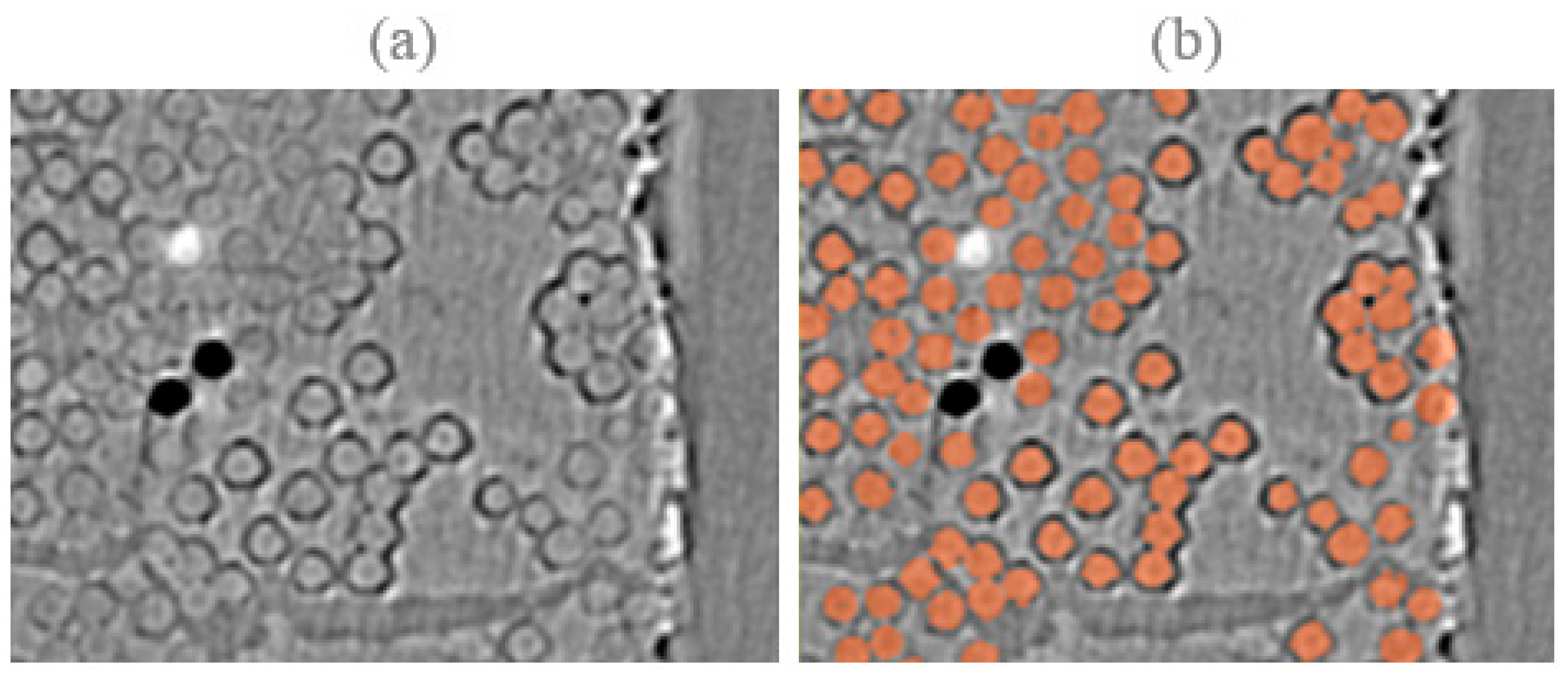
After the completion of testing, the specimen was sectioned and polished normal to the load axis, sequentially at three different locations along the axis. At each location, high-resolution optical images were captured and stitched together to form a complete cross-sectional image (Figure 1a). The CT slice corresponding to each of these optical images was aligned manually with the optical image (Figure 1b,c).
The CT image was obtained before the test specimen was loaded to failure, whereas the optical image was obtained after failure. Damage that occurred during loading after the CT image was obtained can be seen in (a) and (b): gaps (black filled circles) remaining where fibers broke at locations coinciding with the plane of the cross-section and cracks normal to the plane of the cross-section near the left end of the image in (a).
The optical image, with pixel size 0.17 µm, reveals more detailed microstructural information than the lower-resolution CT image (Figure 2).
Figure 1.
(a) Optical image of cross-section of test specimen. (b) Enlargement of area indicated in (a). (c) CT image slice from same area as in (b). The CT image was obtained before the test specimen was loaded to failure, whereas the optical image was obtained after failure. Damage that occurred during loading after the CT image was obtained can be seen in (a,b): gaps (black filled circles) remaining where fibers broke at locations coinciding with the plane of the cross-section and cracks normal to the plane of the cross-section near the left end of the image in (a).

Figure 2.
(a) Optical, (b) CT. Higher magnification images of an area from Figure 1a, with grey level profiles along lines indicated. Pixel sizes: 0.17 µm/pixel in optical image; 1.3 µm/pixel in CT image.
Figure 2.
(a) Optical, (b) CT. Higher magnification images of an area from Figure 1a, with grey level profiles along lines indicated. Pixel sizes: 0.17 µm/pixel in optical image; 1.3 µm/pixel in CT image.

The optical image reveals that BN coatings around the fibers have a variable thickness between 0.2 and 4 μm (varying both around a given fiber and between different fibers), whereas the lower-resolution CT images show no clear difference in widths of thick and thin coatings. However, there is a clear trend of thicker coatings in the optical image corresponding with darker coatings in the CT image, as illustrated by the grey level profiles in Figure 3.
The correlation between coating width and minimum grey level in radial profiles such as Figure 3 is assessed in Section 3.2 as a potential method for measuring coating thickness from the CT image. The optical image also shows that the SiC matrix contains a small amount of silicon, both in isolated islands of diameter less than ~1 μm and in irregular connected channels of width up to ~10 μm. The channels are also visible in the CT image, whereas the isolated islands of silicon are not resolved in the CT image. We also note that the presence of the isolated islands of silicon in the matrix does not alter the average X-ray absorption in the matrix sufficiently to give significant grey level contrast between the fibers and matrix in the CT image. However, in the optical image, there is clear grey level contrast between fibers and matrix.
The images in Figure 1 also show non-uniformity in the spatial distribution of fibers, corresponding with the locations of plies, and a consistent correlation between variations of fiber coating thickness and location within the plies (thicknesses being smaller near the center of the plies than near the exterior). To determine whether these microstructural variations might influence the mechanical behavior and damage of CMCs, it is necessary to quantify the deviations from an ideal composite microstructure having perfectly aligned, uniformly distributed fibers with uniform coatings.
3. Analysis Methods
3.1. Image Segmentation and Correlation
Segmentation of CT images was carried out with a deep learning method based on a convolutional neural network (CNN) in image processing software supplied by Object Research Systems (ORS Dragonfly, Montreal, QC, Canada) (described in [18]). The deep learning model (U-Net architecture) was trained using one cross-sectional image slice that was manually labeled by highlighting pixels associated with fibers. The training slice was taken from the image recorded at the highest load before failure of the composite, after extensive cracking of the matrix and fibers had occurred, in order to train the deep learning model to segment fibers while avoiding matrix cracks and fiber breaks (see Figure A1). Note that the focus of the present study is on the segmentation of fibers from the remainder of the image; the same model has also been trained separately to segment matrix cracks and fiber breaks [18]. Details on the deep learning model training parameters are in the Appendix A. The deep learning model was then used to segment all nine image stacks scanned within the gauge section during the in situ loading experiment, a Hough transform plugin (developed in ImageJ by UCB vision sciences under the GNU Public License) in ImageJ being used to extract the center locations of fibers by finding elliptical features in the segmented CT image. The fibers highlighted in orange in Figure 4 are a result from this automated fiber segmentation from the slice of a CT image recorded at an early stage of the loading (100 MPa) from the location corresponding to one of the high-resolution optical images captured after failure.
The segmentation of the optical image was done by conventional image thresholding, since as noted earlier; there is a grey level difference between fibers, coatings, and matrix. The thicknesses of the fiber coatings were then measured as described in [29]. The segmented fibers of the optical image are shown in black in Figure 4c–e.
Locations of individual fibers in the segmented CT and optical images were matched to allow fiber-to-fiber correlation for comparing the detection rate of the deep learning segmentation. Figure 4 shows the correlation of segmented fibers from the optical images (black) and the segmented fibers from the CT image (orange) with a green line joining the matched fibers centers. The correlation between the locations of segmented fibers in the optical and CT images accounts for relative displacements due to possible misalignment between the CT and optical images (e.g., due to a slight tilt (up to ~0.7°) in the sample while polishing or a tilt while CT or optical imaging). In this manner, fibers that were within ~7 µm in the CT image from their corresponding fibers in the optical image were matched, Figure 4c–e. A full view of the cross-sectional image of the fibers in the optical and CT images with their corresponding segmentation is given in Figure A2.
3.2. Measurements of Fiber Coating Thicknesses
After locating the center of each fiber in the CT image slice and corresponding optical image, profiles of grey level in the image along a set of fiber radii at 48 equally spaced angles were averaged to obtain a location and magnitude for an averaged minimum grey level for the coating surrounding that fiber in the CT image. Typical results for three fibers with coatings of different thicknesses, spanning the range of thicknesses observed in the optical image, are shown in Figure 3. There is a clear correlation in these three cases between the magnitude of the minimum grey level and the average coating thickness obtained from the optical images, with the average minimum grey level varying by more than a factor of two between the fibers with the thickest and thinnest coatings. Results of a detailed correlation for all of the fibers in the three optical images are given in Section 4.2.
The accuracy with which the fiber radii can be measured from the CT image is determined by the accuracy of locating the edge of a fiber, which is limited by contributions to the image contrast from the presence of the coating (of unknown variable thickness below the resolution of the image) and by near-field diffraction effects, which are influenced by scan parameters including the distance between the detector and test specimen. An approach for improving the accuracy of locating the fiber edge by making use of the location and magnitude of the minimum grey level in the average radial profile could be potentially used to improve measurements of fiber radii.
4. Results
4.1. Deep Learning Segmentation Validation
Validation of the deep learning segmentation (DL) involves a comparison between the segmented image and a reference image or “ground truth” (GT). Here, we compare the validation results obtained using three different ground-truth images: the first is a synthetically generated image; the second a manually segmented CT image; and the third a threshold segmented optical image with relatively high resolution from a polished cross-section at the same location as the CT slice.
Various metrics are explored for quantifying the detection rates of fibers using the three validation approaches. Pixel-based metrics for image validation rely on correctly labeled pixels in an image assuming that pixels are a true representation of material phases in the image and are not affected by image noise or artifacts. Although pixel-based metrics are essential in the image training and validation stage, other validation methods based on identifying physical features of the material are needed to relate the accuracy of segmentation to the true structure of materials (which can sometimes be misrepresented by pixel-based methods due to limitations in the resolution). The presence of diffraction effects mentioned in the previous section is an example of how image contrast and edge location can be influenced by scan parameters and thus influence the accurate representation of material phases in the pixels of an image. Material-based metrics such as fiber detection rate do not rely on image pixels for ground truth. The fiber detection rate is a metric based on feature identification and is defined as the number of fibers segmented correctly in the CT images by the deep learning divided by the number of fibers in the ground truth, which may not be sensitive to mislabeling of some of the pixels. Pixel-based metrics on the other hand are a function of all possible outcomes for all the pixels: (i) true positive (TP, number of correctly labeled fiber pixels), (ii) false positive (FP, number of incorrectly labeled fiber pixels), (iii) true negative (TN, number of pixels correctly labeled background), and (iv) false negative (FN, number of pixels incorrectly labeled as background). Different pixel-based metrics are commonly used: (i) Intersection Over Union (IOU) is the area of TP segmented fibers divided by the area of the union of the DL segmented fibers and the fibers in the GT; (ii) the DICE score is two times the area of TP segmented fibers divided by the sum of the number of pixels in the DL and GT; (iii) accuracy is the percentage of correctly labeled pixels in the DL segmentation compared to all labeled pixels; (iv) precision is the ratio of correctly predicted pixels of fibers to the total number of predicted pixels in the DL; (v) recall is the ratio of correctly predicted pixels of fibers in the DL to the ground-truth pixels of fibers. Equations for these validation metrics are as follows:
4.1.1. Ground Truth from Synthetic Data
In this section, the fiber detection rate and pixel-based accuracy of the DL model to segment synthetically generated images of fiber-reinforced composites are assessed using image data from Creveling et al. [19]. Synthetic images were generated to resemble real X-ray CT images of a carbon/epoxy laminate in different pixel sizes and resolutions while accounting for image artifacts and noise [30]. A DL model was trained on one synthetically generated composite image as shown in Figure 5a. The U-Net model training parameters were kept identical to the ones used for the CT images in this study as described in Appendix A. After being trained, the DL model was used to segment all image slices from the synthetic dataset for validation.
The detection rate of the DL model to segment fibers in the synthetic data is 100% (Figure 5b), while the five pixel-based metrics fall in the range of 99.5–100% (Table 1).
All of the errors result from a few incorrectly labeled pixels (FP + FN) at the edges of some fibers, as shown in Figure 5c. These could be due to fiber edges that intersect only part of a pixel and therefore are classified as a fiber pixel. Overall, the DL model successfully trained and segmented the synthetically generated images with a 100% fiber detection rate.
4.1.2. Ground Truth from Manually Segmented CT Images
A ground-truth image was prepared by manually segmenting a region of a CT image slice (621 × 549 pixels) in Figure 1b, shown in Figure 6.
Manual segmentation can be conducted by selecting the pixels of fibers in an image with image highlighting tools in any image processing software (Dragonfly, in this case). The manually segmented image was not used in the training of the DL model so it could provide an unbiased evaluation of the performance of the model. The training of the U-Net model was carried out using a manually trained 549 × 2560 pixel image as described in the Appendix A. The DL model was run to segment the images from all loads including the manually segmented region used for ground truth in Figure 6.
Comparison of the image slice segmented by the trained DL model to the ground-truth image slice yielded a fiber detection rate of 89.6%. Only the TP pixels of the DL segmented fibers were used for the estimate of the detection rate. The intersected pixels between the manually defined ground truth and the segmentations (colored green, Figure 6) are the correctly labeled fibers (TP). Fibers that were in the ground-truth image but missed by the DL segmentation are colored blue (FN). The yellow pixels were erroneously segmented by the DL model as fibers (FP). The reasons for the FN and FP cases are discussed in Section 5. The pixel-based accuracy scores, which ranged from 76% to 94% (Table 1), are much lower than those for the validation method that used ground truth from the synthetic data. Although the variation of scores in Table 1 provides insight to the precision, recall, and accuracy of the DL model, the question is raised as to which pixel-based accuracy score is the most relevant in this case. Since the main objective is to detect and measure fiber locations reliably, validation metrics based on pixels might not be the best indication of segmentation accuracy when the goal is to relate fiber locations to material properties.
4.1.3. Ground Truth from High-Resolution Optical Images
The high-resolution optical image that was segmented by grey level thresholding was used as ground truth to assess the fiber detection rate from the deep learning segmentation of CT images. The DL U-Net model was trained using manually highlighted images as described in the Appendix A. Since the fiber coating plays a key role in distinguishing fibers from the matrix in these CT images, and fibers with the thinnest coatings can be difficult to identify, either by eye or by automated segmentation techniques (Figure 1), use of the high-resolution optical image as ground truth is expected to be the preferred approach.
Superposing the segmented fibers from the CT image onto the optical image, as in Figure 4, allows visual evaluation of the effectiveness of automated segmentation to identify fibers in CT images. The detection rate of the DL segmentation is 93.7%. To assess whether the detection rate is influenced by microstructural parameters such as fiber radius, coating thickness, and fiber location, the combined numbers of fiber detections and misses for all three optical images (total of 2966 fibers) are plotted as a function of these parameters in Figure 7.
The total number of fibers in the optical image with certain radii, coating thicknesses, and locations are shown as grey bars in Figure 7. The red bars represent the subset of the fibers in the optical image that were matched with their corresponding DL segmented fibers from the CT image (detected by CT). Fibers from the optical image with no matched fibers from the CT images (missed by CT) are shown as blue bars. The detection rate does not appear to be dependent on the fiber radius (Figure 7a), whereas it is affected by the coating thickness (Figure 7b), with a bias for fibers with thin coatings being missed by the DL segmentation. In direct examination of images such as Figure 1, it is clear that some of the fibers with thin coatings are challenging to distinguish from the matrix because the dark rings around the fibers become less distinct as the coating thickness decreases.
The fiber detection rate was also plotted as a function of the locations of the fibers within the image, left to right Figure 7c and top to bottom Figure 7d. There is no obvious variation in fiber detection rate across the image from left to right in Figure 7c. However, a bias towards missed fibers being located in the centers of the plies is evident in Figure 7d. This is consistent with the result in Figure 7b (fibers with thin coatings being missed) since the fibers with the thinnest coatings tend to be located in the centers of the plies. Additionally, many fibers at the edges of the cross-section were missed by the DL segmentation (Figure 7d). This is attributed to the presence of image artifacts at the edge of the test specimen as well as damage introduced during preparation of the polished cross-sections for optical imaging (fibers that are chipped or have no matrix around them). In calculating the detection rate listed in Equation (1), fibers along the edges were removed from consideration to avoid these artifacts. If the fibers at the edges were to be included, the detection rate would drop from 93% to 89%. The precision, recall, DICE, and IOU metrics were also evaluated for the validation with ground truth from the optical image as shown in Equations (2)–(6); however, in this case, all TP, FP, FN were considered as numbers of fibers in the CT data. The accuracy metric is not applicable in this case since TN does not apply to fibers as it applies to pixels.
4.2. Calibration of CT Measurements of Coating Thickness with Optical Measurements
After matching the fibers in the three optical cross-section images and the corresponding CT image slices, an averaged minimum grey level for the coating surrounding each fiber in the CT images was computed as described in Section 3.2 and plotted as a function of the average coating thickness measured directly from the corresponding optical image of the fiber. The results are shown in Figure 8.
A consistent inverse relation is evident between the averaged minimum grey level and the coating thickness. A linear regression analysis indicated a correlation with an R2 value of 0.75. With the linear fit to the data shown in Figure 8, the coating thickness can be inferred from a measured grey level with an accuracy of about ±0.5 μm.
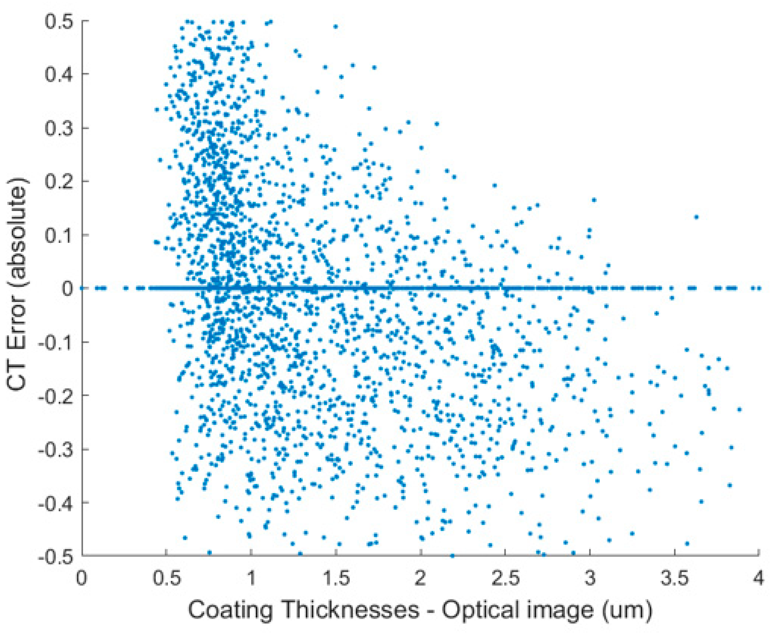
The error of the correlation was evaluated by the difference between the CT and optical coating thickness measurements divided by the absolute value of the optical (CT-Optical)/Optical, shown in Figure A3.
5. Discussion
The validation of DL segmentation of CMCs has been examined using three different approaches for defining ground-truth images.
5.1. Ground Truth from Synthetic Data
Validation based on synthetic images as ground truth is the most accurate approach for benchmarking and comparing the performance of segmentation algorithms (Equations (2)–(6)). However, we note that synthetic datasets are not ideal for validating the segmentation of real images of the composite studied here. Synthetic images may be the best for a more simple composite microstructure as in the graphite–epoxy composite used by Creveling et al. Generation of synthetic data to replicate real images requires considerable expertise and time that may exceed the effort involved with manual labeling of real images and can fail to include all microstructural variations and artifacts found in real images. The synthetic data used here (from Creveling et al. [30]) do not account for statistical variations in microstructural features such as the thickness of fiber coatings, which has a major effect on the details of the image feature used to identify fibers in the composite of this study. For this reason, the use of synthetic data for training followed by validation with real images was not undertaken.
5.2. Ground Truth from Manually Segmented Images
Visual inspection of the manually labeled ground-truth image in Figure 6 reveals that most of the false negatives were fibers with thin coatings that were not detected in the automated segmentation. The false positives were either (1) artifacts in the image that had groups of pixels with relatively low grey levels arranged in a ring shape that resembled a fiber, or in a few cases fibers that were missed by the manual labeling of the ground-truth image. The potential for missing or mislabeling ground-truth pixels due to human errors is a drawback of this validation method. However, the use of manually trained ground-truth images remains the most convenient and accessible method for generating diverse training data that encompass most variations in an image. Although the success of a deep learning model relies on the quality of the ground-truth image, the human errors in the training image, if sufficiently rare, can be treated as outliers in the training set and given less weight by the deep learning training procedure. This leads to successful networks that can learn to segment fibers with thin coatings, even if there are misses in the manually segmented ground-truth images.
5.3. Ground Truth from High-Resolution Optical Images
The use of a higher-resolution image as ground truth, an optical image in this case, allows for a more accurate evaluation of the segmentation performance than the use of ground truth from manually labeled CT images or synthetically generated data. Similar to the validation method using GT from manually segmented images, a fiber detection rate is evaluated by comparing the fibers segmented by deep learning to their corresponding matched fibers in the optical image. However, there are no labeling errors in the optical validation method.
The detection rate metric gives more insight on the performance of the segmentation because it relies on a one-to-one fiber detection correlation instead of an accuracy based on overlapping pixels. In Figure 9, there is a clear correlation between missed fibers and fibers with thin coatings.
This is another visual evidence of the dependence of the DL model detection rate on the fiber coating thickness. The effect of image distortion on the edge of the sample, seen in Figure 9, can cause the DL segmentations to miss fibers. In addition, reconstruction artifacts can distort the circularity of the fibers in the CT image, shown in the missed fibers of Figure 9. Fibers in the CT images are observed to have deviations from circularity, shown clearly in Figure 3a–c. This deviation is due to shifting in the center of image reconstruction.
5.4. Measurements from CT Image
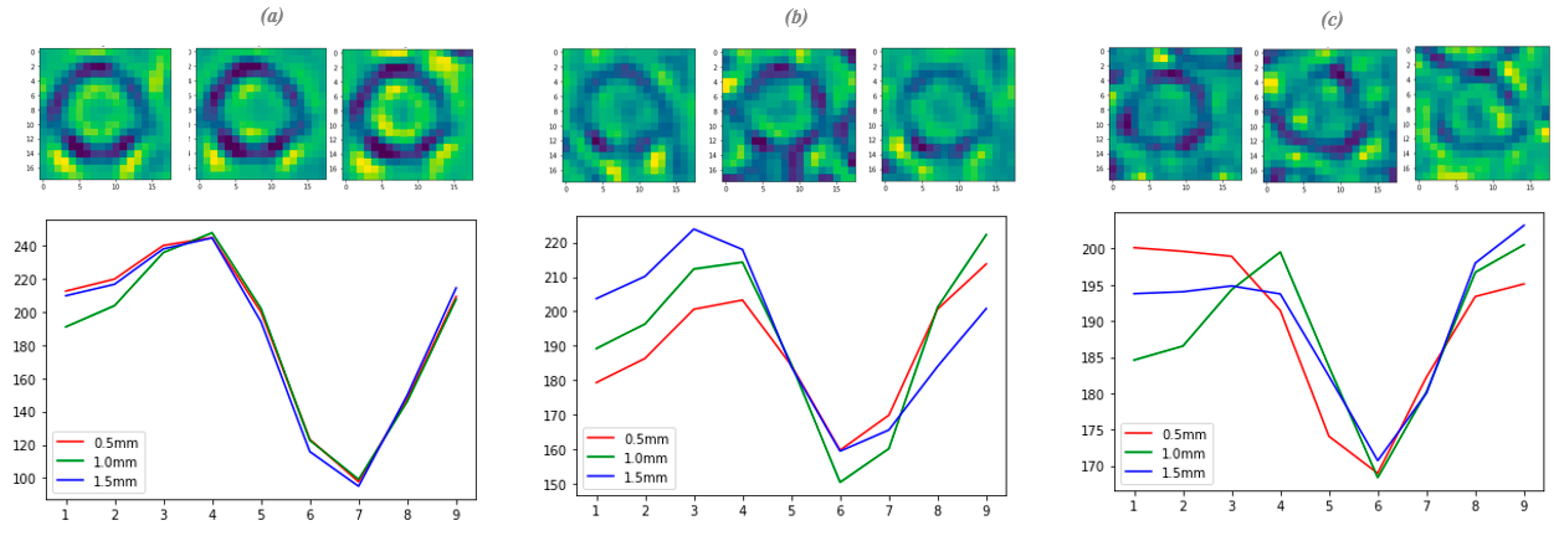
The correlation shown in Figure 8 between minimum grey level in the coating image and coating thickness enables assessment of the uniformity of coating thickness along the lengths of individual fibers. The coating thickness was computed using this approach at several locations along each fiber within the 3 mm field of view of the CT images. Examples are shown for three fibers with coatings of different thickness, one representative of the thickest coatings, one of medium thickness and one representative of the thinnest coatings, as shown in Figure 10.
The radial profiles and the minimum grey level values are almost identical along a given fiber, indicating that the fiber coating thicknesses do not vary greatly along the fiber length.
6. Conclusions
Segmentation training and validation using synthetic images provide higher accuracy than other training and validation methods. Consequently, synthetic images are commonly used for benchmarking segmentation algorithms [31,32]. However, expertise and time are required to generate synthetic images including noise and artifacts. Any variations in material constituents or imaging parameters would require generation of new synthetic replicas for training. Manually labeled CT image slices for DL model training are more accessible and easier to use. However, validation with manually defined ground truth is not ideal because of the human errors introduced. In this work, validation of image segmentation with ground truth defined by a higher-resolution optical image resulted in an accurate assessment of fiber detection rate compared to the physical sample, instead of solely relying on an image-based verification method. Although validation methods relying on high-resolution images can be laborious in some cases, they provide a more accurate assessment of detection rates and measurements.
Measurements of sub-pixel features in images are feasible but only limited to a relative minimum grey level difference that could be calibrated in the presence of a ground truth from a high-resolution image. The superior resolution of the optical image allowed for accurate measurements and a one-to-one correlation with estimates extracted from CT. Coating thickness measurements from the CT images were directly correlated to measurements from the optical image. In this work, the minimum grey level value of the fiber radial profile correlated with coating thickness measurements from the high-resolution optical image has an R2 value of 0.75. This demonstrated that it is possible to estimate measurements of features below the resolution of CT while validating and calibrating estimates with a higher-resolution image. The calibrations carried out for the measurements in this work are limited to images from similar material with identical scan parameters. However, the methodology for extracting relative measurements from sub-pixel features can be adapted to other images. The segmentations and measurements from this work have been used to study the effect of microstructural variability on matrix cracking and fiber fracture in this class of SiC–SiC composites [33].
Author Contributions
Conceptualization, A.B., D.P., D.U. and E.M.; formal analysis, A.B. and D.P.; funding acquisition, E.M. and D.M.; methodology, A.B., D.P., D.U. and D.M.; software, A.B., D.P. and E.M.; supervision, D.M. and E.M.; validation, D.M.; visualization, A.B., D.M. and E.M.; writing—original draft, A.B.; writing—review & editing, D.M., D.U. and E.M. All authors have read and agreed to the published version of the manuscript.
Funding
A US National Science Foundation PIRE program at Kansas State University, Grant number 1743701, funded this work. The materials and experiments that provided the images analyzed in this paper were supported by the AFRL under contract F865011C5227. This work was performed as part of an approved program at the Advanced Light Source (Lawrence Berkeley National Laboratory, Berkeley, CA, USA), which is a DOE Office of Science User Facility [contract no. DE-AC02-05CH11231].
Institutional Review Board Statement
Not applicable.
Informed Consent Statement
Not applicable.
Data Availability Statement
The deep learning models for segmentation can be downloaded from the Materials Data Facility Repository [34]. The codes for image correlation and radial profile can be downloaded from the same repository.
Acknowledgments
The authors would like to thank A. Santamaria-pang, A. Singhal, and Y. Gao for their technical support in sample preparation, in situ experiments, and optical imaging.
Conflicts of Interest
The authors have no conflict of interest to declare.
Appendix A. Details of Analysis Methods
Appendix A.1. Deep Learning Image Segmentation
A U-Net model (layer depth of 3 and initial filter count of 64) was trained for 77 epochs with early stopping enabled to avoid overfitting (The model stops early if the validation loss increases). Other model parameters were assigned as follows: the input patch and batch size were set to 32; the stride to input ratio was 0.25; the loss function used was ORSDiceLoss, and the optimization algorithm used was adadelta.
From the image used for training (consisting of 549 × 2560 pixels), 60% of the pixels were used for training, 20% were reserved for training validation, and 20% were reserved for test. The training image shown in Figure A1, was augmented to increase the training volume by flipping vertically, horizontally, sheared, rotated and scaled differently at every epoch cycle. Validation and test pixels were reserved, unseen by the model while training, to ensure an unbiased evaluation of model accuracy. These pixels were used by model optimization functions and are kept separate from the manually segmented ground truth used for inference validation in Section 4.1.2. Once the training accuracy reached a DICE accuracy of 89% on the validation dataset the model was used to segment previously unseen image stacks.
Figure A1.
A cropped (a) raw (b) manually labeled CT image used for deep learning training.
Appendix A.2. Hough Transform
A Hough transform was used to find the circular features of the segmented fibers. The segmented images were converted from filled circles of fibers to empty circles with the default edge detection in ImageJ. The Hough transform parameters used for extracting fiber centers and radii were as follows: minimum search radius, 6 pixels; maximum search radius, 10 pixels; radius search increment, 1 pixel; maximum number of circles to be found, 3500; Hough score threshold, 0.7; and the number of steps per transform were 1000. From an input of a binary image of fiber segmentations, an output matrix file of fiber X&Y center location and an estimated fiber radius was extracted.
Figure A2.
(a) Segmented CT cross-sectional image and its corresponding (b) optical image (c) alignment and correlation of optical and CT fiber segmentations optical fibers mask (black), CT fibers (red) and a line (green) joining center coordinates of fibers. The optical fiber to CT Fiber correlation and alignment has a tolerance of matching fibers centers 7 µm apart, to account for possible misalignment between cross-section slice in 3D CT and the sectioned/polished plane in optical.

Figure A3.
Absolute error in the fiber coating thickness correlation (CT-Optical)/Optical.
References
- Bale, H.A.; Blacklock, M.; Begley, M.R.; Marshall, D.B.; Cox, B.N.; Ritchie, R.O. Characterizing three-dimensional textile ceramic composites using synchrotron x-ray micro-computed-tomography. J. Am. Ceram. Soc. 2012, 95, 392–402. [Google Scholar] [CrossRef]
- Bale, H.A.; Haboub, A.; Macdowell, A.A.; Nasiatka, J.R.; Parkinson, D.Y.; Cox, B.N.; Marshall, D.B.; Ritchie, R.O. Real-time quantitative imaging of failure events in materials under load at temperatures above 1600 °C. Nat. Mater. 2013, 12, 40–46. [Google Scholar] [CrossRef]
- Chateau, C.; Gélébart, L.; Bornert, M.; Crépin, J.; Boller, E.; Sauder, C.; Ludwig, W. In situ X-ray microtomography characterization of damage in SiCf/SiC minicomposites. Compos. Sci. Technol. 2011, 71, 916–924. [Google Scholar] [CrossRef] [Green Version]
- Wright, P.; Moffat, A.; Sinclair, I.; Spearing, S.M.; High, S.M.S. High resolution tomographic imaging and modelling of notch tip damage in a laminated composite. Compos. Sci. Technol. 2012, 70, 1444–1452. [Google Scholar] [CrossRef] [Green Version]
- Mazars, V.; Caty, O.; Couégnat, G.; Bouterf, A.; Roux, S.; Denneulin, S.; Pailhès, J.; Vignoles, G.L. Damage investigation and modeling of 3D woven ceramic matrix composites from X-ray tomography in-situ tensile tests. Acta Mater. 2017, 140, 130–139. [Google Scholar] [CrossRef] [Green Version]
- Cox, B.N.; Bale, H.A.; Begley, M.R.; Blacklock, M.; Do, B.-C.; Fast, T.; Naderi, M.; Novak, M.D.; Rajan, V.P.; Rinaldi, R.G.; et al. Stochastic Virtual Tests for High-Temperature Ceramic Matrix Composites. Annu. Rev. Mater. Res. 2014, 44, 479–529. [Google Scholar] [CrossRef]
- Saucedo-Mora, L.; Lowe, T.; Zhao, S.; Lee, P.D.; Mummery, P.M.; Marrow, T.J. In situ observation of mechanical damage within a SiC-SiC ceramic matrix composite. J. Nucl. Mater. 2016, 481, 13–23. [Google Scholar] [CrossRef]
- Barnard, H.S.; MacDowell, A.A.; Parkinson, D.Y.; Mandal, P.; Czabaj, M.W.; Gao, Y.; Maillet, E.; Blank, B.; Larson, N.M.; Ritchie, R.O.; et al. Synchrotron X-ray micro-tomography at the Advanced Light Source: Developments in high-temperature in-situ mechanical testing. J. Phys. Conf. Ser. 2017, 849. [Google Scholar] [CrossRef] [Green Version]
- Larson, N.M.; Cuellar, C.; Zok, F.W. X-ray computed tomography of microstructure evolution during matrix impregnation and curing in unidirectional fiber beds. Compos. Part A Appl. Sci. Manuf. 2019, 117, 243–259. [Google Scholar] [CrossRef]
- Garcea, S.C.; Wang, Y.; Withers, P.J. X-ray computed tomography of polymer composites. Compos. Sci. Technol. 2018, 156, 305–319. [Google Scholar] [CrossRef]
- Mardia, K.V.; Hainsworth, T.J. A Spatial Thresholding Method for Image Segmentation. IEEE Trans. Pattern Anal. Mach. Intell. 1988, 10, 919–927. [Google Scholar] [CrossRef]
- Pham, D.L.; Xu, C.; Prince, J.L. Current Methods in Medical Image Segmentation. Ann. Rev. Biomed. Eng. 2000, 2, 315–337. [Google Scholar] [CrossRef] [PubMed]
- Perciano, T.; Ushizima, D.M.; Krishnan, H.; Parkinson, D.Y.; Larson, N.M.; Pelt, D.M.; Bethel, W.; Zok, F.W.; Sethian, J. Insight into 3D micro-CT data: Exploring segmentation algorithms through performance metrics. J. Synchrotron Radiat. 2017, 24, 1065–1077. [Google Scholar] [CrossRef] [PubMed]
- Straumit, I.; Lomov, S.V.; Wevers, M. Quantification of the internal structure and automatic generation of voxel models of textile composites from X-ray computed tomography data. Compos. Part A Appl. Sci. Manuf. 2015, 69, 150–158. [Google Scholar] [CrossRef]
- Ushizima, D.; Perciano, T.; Krishnan, H.; Loring, B.; Bale, H.A.; Parkinson, D.Y.; Sethian, J. Structure recognition from high resolution images of ceramic composites. In Proceedings of the 2014 IEEE International Conference on Big Data, Washington, DC, USA, 27–30 October 2014; pp. 683–691. [Google Scholar] [CrossRef] [Green Version]
- Czabaj, M.W.; Riccio, M.L.; Whitacre, W.W. Numerical reconstruction of graphite/epoxy composite microstructure based on sub-micron resolution X-ray computed tomography. Compos. Sci. Technol. 2014, 105, 174–182. [Google Scholar] [CrossRef]
- Emerson, M.J.; Jespersen, K.M.; Dahl, A.B.; Conradsen, K.; Mikkelsen, L.P. Individual fibre segmentation from 3D X-ray computed tomography for characterising the fibre orientation in unidirectional composite materials. Compos. Part A Appl. Sci. Manuf. 2017, 97, 83–92. [Google Scholar] [CrossRef]
- Badran, A.; Marshall, D.B.; Legault, Z.; Makovetsky, R.; Provencher, B.; Piché, N.; Marsh, M. Automated segmentation of computed tomography images of fiber-reinforced composites by deep learning. J. Mater. Sci. 2020, 55, 16273–16289. [Google Scholar] [CrossRef]
- Creveling, P.J.; Whitacre, W.W.; Czabaj, M.W. A fiber-segmentation algorithm for composites imaged using X-ray microtomography: Development and validation. Compos. Part A Appl. Sci. Manuf. 2019, 126, 105606. [Google Scholar] [CrossRef]
- Sinchuk, Y.; Kibleur, P.; Aelterman, J.; Boone, M.N.; Paepegem, W. Van Geometrical and Deep Learning Approaches for Instance Segmentation of CFRP Fiber Bundles in Textile Composites. Compos. Struct. 2021, 277, 114626. [Google Scholar] [CrossRef]
- Emerson, M.J.; Dahl, V.A.; Conradsen, K.; Mikkelsen, L.P.; Dahl, A.B. Statistical validation of individual fibre segmentation from tomograms and microscopy. Compos. Sci. Technol. 2018, 160, 208–215. [Google Scholar] [CrossRef]
- Padture, N.P. Advanced structural ceramics in aerospace propulsion. Nat. Mater. 2016, 15, 804–809. [Google Scholar] [CrossRef] [PubMed]
- Zok, F.W. Ceramic-matrix composites enable revolutionary gains in tubeine engine efficiency. Am. Ceram. Soc. Bull. 2016, 95, 22–28. [Google Scholar]
- Spitsberg, I.; Steibel, J. Thermal and Environmental Barrier Coatings for SiC/SiC CMCs in Aircraft Engine Applications. Int. J. Appl. Ceram. Technol. 2004, 1, 291–301. [Google Scholar] [CrossRef]
- Steibel, J. Ceramic Matrix Composites Taking Flight at GE Aviation, (n.d.). Available online: www.ceramics.org (accessed on 16 September 2021).
- Hilmas, A.M.; Sevener, K.M.; Halloran, J.W. Damage evolution in SiC/SiC unidirectional composites by X-ray tomography. J. Am. Ceram. Soc. 2020, 103, 3436–3447. [Google Scholar] [CrossRef]
- Maillet, E.; Singhal, A.; Hilmas, A.M.; Gao, Y.; Zhou, Y.; Henson, G.; Wilson, G. Combining in-situ synchrotron X-ray microtomography and acoustic emission to characterize damage evolution in ceramic matrix composites. J. Eur. Ceram. Soc. 2019, 39, 3546–3556. [Google Scholar] [CrossRef]
- Haboub, A.; Bale, H.A.; Nasiatka, J.R.; Cox, B.N.; Marshall, D.B.; Ritchie, R.O.; Macdowell, A.A. Tensile testing of materials at high temperatures above 1700 °C with in situ synchrotron X-ray micro-tomography. Rev. Sci. Instrum. 2014, 85, 1–13. [Google Scholar] [CrossRef] [Green Version]
- Brada, R.S.; Ron Wein, R.; Wilson, G.; Santamaria-Pang, A.; Gugel, L. Multi-Stage Segmentation using Synthetic Images. U.S. Patent 10991101, 27 April 2021. [Google Scholar]
- Creveling, P.J.; Whitacre, W.; Czabaj, M. Synthetic X-ray Microtomographic Image Data of Fiber-Reinforced Composites. 2019. Available online: https://materialsdata.nist.gov/handle/11256/988 (accessed on 9 June 2021).
- Ros, G.; Sellart, L.; Materzynska, J.; Vazquez, D.; Lopez, A.M. The Synthia Dataset: A Large Collection of Synthetic Images for Semantic Segmentation of Urban Scenes. In Proceedings of the IEEE Conference on Computer Vision and Pattern Recognition, Las Vegas, NV, USA, 27–30 June 2016; pp. 3234–3243. [Google Scholar]
- Hinterstoisser, S.; Lepetit, V.; Wohlhart, P.; Konolige, K. On Pre-Trained Image Features and Synthetic Images for Deep Learning. In Proceedings of the European Conference on Computer Vision (ECCV) Workshops 2018, Munich, Germany, 8–14 September 2018. [Google Scholar]
- Badran, A.; Marshall, D.B.; Maillet, E. Effect of Microstructural Variability on Matrix Cracking and Fiber Fracture in Unidirectional SiC-SiC Composites. Unpublished work. 2022; in preparation. [Google Scholar]
- Badran, A.; Marshall, D.B.; Legault, Z.; Makovetsky, R.; Provencher, B.; Piché, N.; Marsh, M. XCT dataset and Deep Learning Models for Automated Segmentation of Computed Tomography Images of Fiber-Reinforced Composites. Mater. Data Facil. Open 2020. [Google Scholar] [CrossRef]
Figure 3.
CT images of three fibers with coatings of different thicknesses spanning the range seen in Figure 1b (thickest in (a), medium in (b) and thinnest in (c)). (d) Radial grey level profiles for each fiber averaged over a set of 48 radial lines obtained by rotating the line indicated in red (a) about the center of the fiber in increments of 2π/48.

Figure 4.
Comparisons of segmented fibers with optical image of an area within Figure 1a. (a) Optical image. (b) Superposition of optical image in (a) with fiber segmentation mask derived from CT image of the same area. (c–e) Superposition of fiber segmentation masks derived from optical image (black) and CT image slice (red). Green lines connect corresponding fibers in the two masks (the correlation allowed a tolerance up to 7 µm to account for possible misalignment between the optical and CT images).

Figure 5.
Superposition of synthetic image with (a) ground-truth segmentation (GT, blue) and (b) deep learning segmentation (DL, orange). Locations of false positives (FP) and false negatives (FN) are indicated by yellow pixels in (c).
Figure 5.
Superposition of synthetic image with (a) ground-truth segmentation (GT, blue) and (b) deep learning segmentation (DL, orange). Locations of false positives (FP) and false negatives (FN) are indicated by yellow pixels in (c).

Figure 6.
Superposition of CT image with two segmentations: (i) ground-truth segmentation (GT) obtained by manual segmentation of the CT image and (ii) deep learning segmentation (DL). Green = intersection of DL and GT; yellow = fibers identified by DL but not in GT (FP); blue = fibers in GT but missed by DL (FN).
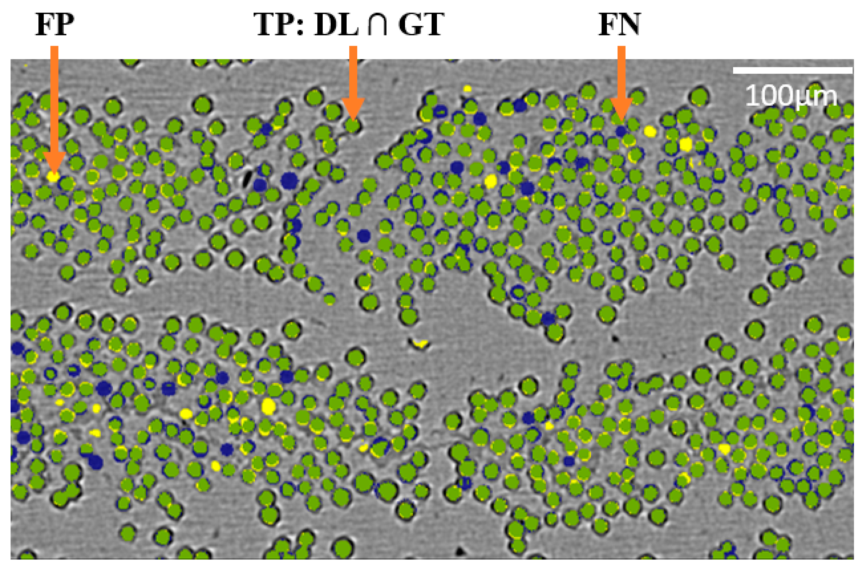
Figure 7.
Fiber detection rates as a function of (a) fiber radius, (b) coating thickness, (c) location in horizontal direction in the image of Figure 1 (x-coordinate), and (d) location in vertical direction in the image of Figure 1 (y-coordinate). The combined detection rate is 93.7%. In (a) missed fibers are not correlated with variations in fiber radii. In (b) fibers with thin coatings are more likely to be missed. In (d) most of the missed fibers are located in the centers of the plies.
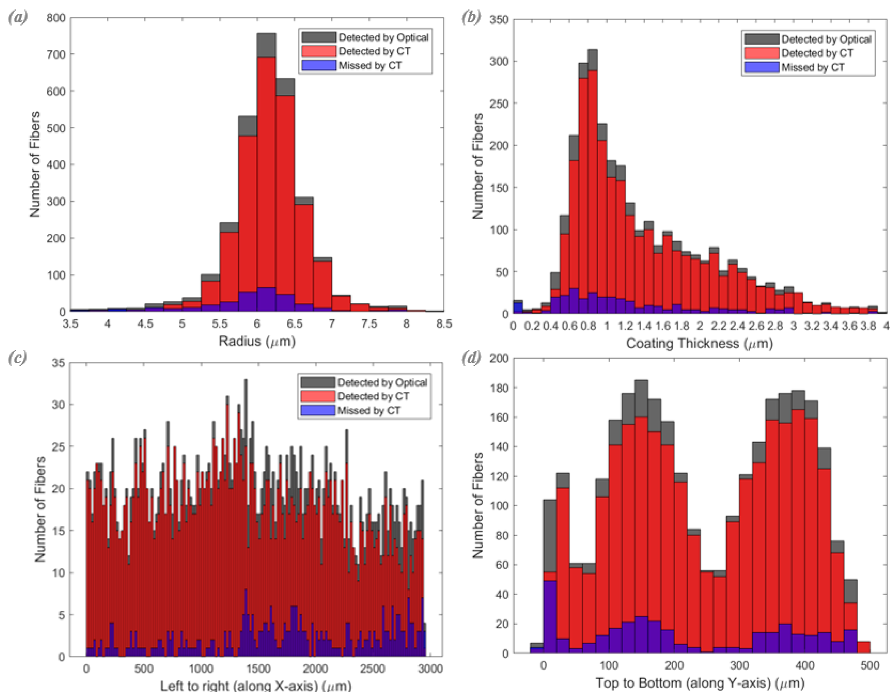
Figure 8.
Correlation between minimum grey level in averaged radial profile for each fiber in CT image and thickness of fiber coating obtained from optical image.
Figure 8.
Correlation between minimum grey level in averaged radial profile for each fiber in CT image and thickness of fiber coating obtained from optical image.
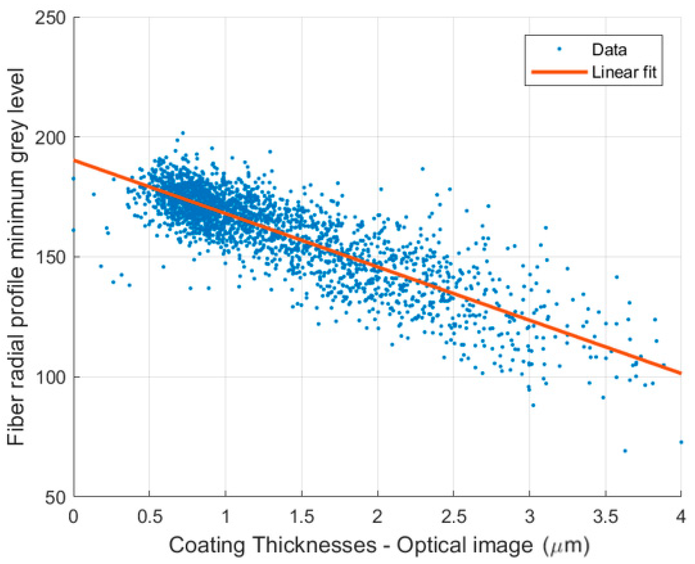
Figure 9.
Higher magnification views of images and segmentations from a small region within Figure 3, showing the effect of damage and image artifacts near the edge of the test specimen: (a) optical image; (b) CT image; (c) superposition of fiber segmentation masks derived from optical image (black) and CT image slice (red). Green lines connect corresponding fibers in the two masks.

Figure 10.
CT images and radial grey level profiles from three fibers with coatings of different thickness at three locations along the length of each fiber: (a) coating of high thickness; (b) coating of medium thickness; and (c) coating of low thickness.
Figure 10.
CT images and radial grey level profiles from three fibers with coatings of different thickness at three locations along the length of each fiber: (a) coating of high thickness; (b) coating of medium thickness; and (c) coating of low thickness.

Table 1.
A comparison between three segmentation validation methods.
| Metric | ||||||
|---|---|---|---|---|---|---|
| Method | Detection Rate % | Precision % | Recall % | Accuracy % | DICE % | IOU % |
| Synthetic | 100 | 99.8 | 99.6 | 100 | 99.7 | 99.5 |
| GT from Manual | 89.6 | 93.9 | 86.5 | 76.2 | 93.3 | 80.6 |
| GT from Optical | 93.7 | 88.4 | 89.2 | NA | 88.8 | 80.0 |
Publisher’s Note: MDPI stays neutral with regard to jurisdictional claims in published maps and institutional affiliations. |
© 2022 by the authors. Licensee MDPI, Basel, Switzerland. This article is an open access article distributed under the terms and conditions of the Creative Commons Attribution (CC BY) license (https://creativecommons.org/licenses/by/4.0/).
Share and Cite
MDPI and ACS Style
Badran, A.; Parkinson, D.; Ushizima, D.; Marshall, D.; Maillet, E. Validation of Deep Learning Segmentation of CT Images of Fiber-Reinforced Composites. J. Compos. Sci. 2022, 6, 60. https://doi.org/10.3390/jcs6020060
AMA Style
Badran A, Parkinson D, Ushizima D, Marshall D, Maillet E. Validation of Deep Learning Segmentation of CT Images of Fiber-Reinforced Composites. Journal of Composites Science. 2022; 6(2):60. https://doi.org/10.3390/jcs6020060
Chicago/Turabian StyleBadran, Aly, Dula Parkinson, Daniela Ushizima, David Marshall, and Emmanuel Maillet. 2022. "Validation of Deep Learning Segmentation of CT Images of Fiber-Reinforced Composites" Journal of Composites Science 6, no. 2: 60. https://doi.org/10.3390/jcs6020060