Machining Forces Due to Turning of Bimetallic Objects Made of Aluminum, Titanium, Cast Iron, and Mild/Stainless Steel

Ullah, AMM Sharif

doi:10.3390/jmmp2040068

Open AccessArticle

Machining Forces Due to Turning of Bimetallic Objects Made of Aluminum, Titanium, Cast Iron, and Mild/Stainless Steel

by

AMM Sharif Ullah

Faculty of Engineering, Kitami Institute of Technology, Kitami 090-8507, Japan

J. Manuf. Mater. Process. 2018, 2(4), 68; https://doi.org/10.3390/jmmp2040068

Submission received: 28 August 2018 / Revised: 5 October 2018 / Accepted: 10 October 2018 / Published: 11 October 2018

(This article belongs to the Special Issue Anniversary Feature Papers)

Download

Browse Figures

Versions Notes

Abstract

:

This article elucidates the characteristics of machining forces (an important phenomenon by which machining is studied) using three sets of bimetallic specimens made of aluminum–titanium, aluminum–cast iron, and stainless steel–mild steel. The cutting, feed, and thrust forces were recorded for different cutting conditions (i.e., different cutting speeds, feeds, and cutting directions). Possibility distributions were used to quantify the uncertainty associated with machining forces, which were helpful in identifying the optimal machining direction. In synopsis, it was found that while machining the steel-based bimetallic specimens, keeping a low feed and high cutting speed is the better option, and the machining operation can be performed in both the hard-to-soft and soft-to-hard material directions, but machining in the soft-to-hard material direction is the better option. On the other hand, very soft materials should not be used in fabricating a bimetallic part because it creates machining problems. Cutting power was estimated using the cutting and feed force signals. Manufacturers who support sustainable product development (including design, manufacturing, and assembly) can benefit from the outcomes of this study because parts/products made of dissimilar materials (or multi-material objects) are better than their mono-material counterparts in terms of sustainability (cost, weight, and CO₂ footprint).

Keywords:

sustainability; bimetallic object; cutting force; uncertainty; machining power

1. Introduction

The research on machining is mostly concerned with the machining of objects made of mono-material and special alloys. On the other hand, research on the machining of objects made of multiple materials cannot be ignored, mainly because of the rising concerns for sustainability. The explanation is given below.

In general, sustainability means fulfilling the present generation’s needs without compromising the ability to fulfill the future generations’ needs [1]. In more specific terms, sustainability means ensuring material efficiency, energy efficiency, and component efficiency, preferably simultaneously, for all products that inhabit the artificial world [2]. Here, material efficiency is with respect to the usages of materials and takes into account the issues regarding energy consumption and resource depletion while producing the primary materials; it also considers issues like the cost and weight reduction of a product [2,3,4,5]. Energy efficiency takes into account the energy consumption during the manufacturing activities (e.g., machining and assembly) of a product [2,5]. Component efficiency takes into account the degree of fulfillment of the intended functionality, quality, and reliability requirements of the components used in a product [2]. The interplay of these efficiencies is presented in detail in [2], where it is concluded that material efficiency is more effective than the other two efficiencies in enhancing the sustainability of a product. For example, a multi-material object is better than its monometallic counterpart (e.g., an object made of aluminum–titanium is better than its monometallic counterpart made of Titanium only, in terms of cost, weight, and CO₂ footprint) [2]. Increasing the material efficiency might affect the energy and component efficiencies, which is not desirable. Therefore, optimization is needed to obtain the best that a multi-material object can offer.

Nevertheless, the usages of multi-material products are expected to increase in the years to come due to the fact mentioned above (i.e., enhancing the sustainability of a product from the viewpoint of material efficiency). Nowadays, both physical joining processes (e.g., friction welding) [6,7,8,9] and additive manufacturing processes (e.g., selective laser sintering) [10,11,12,13] are used to manufacture objects made of dissimilar metals. The advent of such manufacturing processes will also accelerate the usages of multi-material products since these processes help manufacture different parts made of different types of dissimilar metals. It is worth mentioning that additive manufacturing processes that add materials layer by layer based on the solid model of an object have been found suitable for manufacturing very complex and highly customized objects using multiple materials [10,11,12,13]. As such, additive manufacturing processes (selective laser sintering) can easily fabricate an object made of multiple materials, which is often difficult to achieve by conventional manufacturing processes (e.g., machining, casting, forming, and welding).

The above explanation refers to the fact that more and more objects made of multiple materials will inhabit our surroundings in the years to come. However, a multi-material object manufactured either by additive manufacturing or by other manufacturing processes (e.g., friction welding) must be machined so that it achieves the required dimensional accuracy and surface finish. This necessitates machining knowledge regarding multi-material objects. In the literature, a relatively limited number of studies are found regarding the machining of objects made of dissimilar materials. In particular, the studies reported in [14,15,16,17,18,19,20,21] are noted. These studies show that the machining of a multi-material object entails some unique properties. For example, a monometallic workpiece can be machined from any sides, whereas while machining a workpiece made of two different materials, the machining direction must be optimized (e.g., machining from the softer material side to the harder material side or vice versa) [20]. The surface roughness quantification process of an object made of two different metals needs some unconventional parameters (e.g., entropy, possibility distribution, and the like) [19,21]. The main issue of such uniqueness is the existence of the joint area or heat-affected zone, where the material compositions and properties (particularly hardness) exhibit a great deal of variability compared to the constituent materials. The authors in [6,7,8,9,22] have described this issue elaborately. Depending on whether a cutting tool passes the joint area from the softer material side to the harder material side, or vice versa, the machining characteristics might differ. As a result, the machining forces (cutting force, feed force, and so on) might exhibit a different kind of character when the cutting tool passes the joint area either from the softer material side to the harder material side or vice versa. Since machining forces provide valuable insights into machining phenomena [23], it is worth investigating the nature of the machining forces that arise when a cutting tool passes the joint area from both sides of a bimetallic specimen. From this contemplation, this article reports the characteristics of machining forces that occur when turning three sets of dissimilar metallic specimens made of aluminum–titanium, aluminum–cast iron, and stainless steel–mild steel. Accordingly, the remainder of this article is organized as follows. Section 2 describes the bimetallic specimens, experimental setup, and data acquisition technique. Section 3 presents the characteristics of the machining forces underlying the stainless steel–mild steel in terms of time series data and uncertainty. Section 4 presents the characteristics of the machining forces underlying the aluminum–titanium in terms of time series data and uncertainty. Section 5 presents the characteristics of the machining forces underlying the aluminum–cast iron in terms of time series data and uncertainty. Section 6 discusses the implication of the results. Section 7 provides the concluding remarks of this study.

2. Machining Experiments and Data Acquisition

This section describes the bimetallic specimens, experimental setup, and data acquisition technique used while turning the bimetallic specimens.

Three different sets of bimetallic specimens were fabricated using friction welding [6,7]. The description of the welding conditions can be found in [2]. Table 1 lists the materials used to prepare the specimens. The tensile strength, percent elongation, and hardness of each material are also listed in Table 1.

The first set of specimens, defined as SU–SC, was prepared by joining two different materials, namely, stainless steel (JIS: SUS304) and mild steel (JIS: S15CK). The chemical composition (wt%) of the stainless steel was as follows: 0.052 C, 0.416 Si, 1.529 Mn, 0.0319 P, 0.0186 S, 8.057 Ni, 18.293 Cr, 0.185 Mo, 0.483 Cu, and 70.9345 Fe. The chemical composition (wt%) of the mild steel was as follows: 0.15 C, 0.20 Si, 0.40 Mn, 0.19 P, 0.022 S, 0.03 Ni, 0.14 Cr, 0.02 Cu, and 98.848 Fe. The tensile strength (i.e., ultimate strength), elongation, and hardness of the stainless steel were 663 MPa, 55%, and 182 HV, respectively. The tensile strength (i.e., ultimate strength), elongation, and hardness of the Mild Steel were 439 MPa, 38%, and 132 HV, respectively. The second set of specimens, defined as Al–Ti, was prepared by joining two different materials, namely, aluminum (JIS: A1070) and commercial pure (CP) titanium. The chemical composition (wt%) of the aluminum (JIS: A1070) were as follows: 0.03 Si, 0.10 Fe, 0.01 Cu, 0.02 Mg, 0.01 V, 0.01 Ti, others ≤ 0.03 others, and 99.82 Al. The chemical composition (wt%) of the CP titanium was as follows: 0.0011 H, 0.089 O, 0.006 N, 0.038 Fe, 0.005 C, and 99.8609 Ti. The tensile strength (i.e., ultimate strength), elongation, and hardness of the aluminum (JIS: A1070) were 120 MPa, 27%, and 41 HV, respectively. The tensile strength (i.e., ultimate strength), elongation, and hardness of the CP titanium were 401 MPa, 35%, and 146 HV, respectively. The other set of specimens, defined as Al–CI, was prepared by joining two different materials, namely, aluminum (JIS: A5052) and ductile cast iron. The chemical composition (wt%) of the aluminum (JIS: A5052) was as follows: 0.09 Si, 0.16 Fe, 0.02 Cu, 0.03 Mn, 2.6 Mg, 0.25 Cr, 0.01 Zn, ≤0.15 others, and 96.69 Al. The chemical composition (wt%) of the ductile cast iron was as follows: 3.76 C, 2.91 Si, 0.49 P, 0.011 S, 0.029 Mg, and 92.8 Fe. The tensile strength (i.e., ultimate strength), elongation, and hardness of the aluminum (JIS: A5052) were 265 MPa, 17.4%, and 86 HV, respectively. The tensile strength (i.e., ultimate strength), elongation, and hardness of the ductile cast iron were 442 MPa, 18.7%, 79.2 HRB, respectively.

Note that the tensile strength, percent elongation, and hardness of one of the constituent materials are greater than those of the other for each set of specimens. This ensures machining of soft-to-hard material or vice versa at the joint area. Figure 1 shows the pictures of the specimens, one from each set of specimens. The flash generated in the joint area (see Figure 1) was removed by using a turning operation before conducting the machining experiments for obtaining the machining force data. The friction welding conditions used to prepare the bimetallic specimens (Figure 2) are listed in Table 2. As seen in Table 2, for the specimens called SU-SC, the rotating material was S15CK (i.e., mild steel). For the specimens called Al-Ti, the rotating material was A1070 (i.e., aluminum). For the other specimens, the rotating material was A5052 (aluminum). The diameters of rotating material (while performing friction welding) for all specimens were 12 mm. The friction speed, friction pressure, and upset time were 27.5 s⁻¹ (1650 rpm), 30 MPa, and 6 s, respectively, for all specimens. Whereas, the friction times for the specimens namely SU-SC, Al-Ti, and Al-CI were 2 s, 1 s, and 3 s, respectively. The upset pressures for the specimens, namely SU-SC, Al-Ti, and Al-CI were 270 MPa, 90 MPa, and 200 MPa, respectively.

On the other hand, the cutting conditions for the machining experiments are summarized in Table 3. Carbide inserts (TNMG160404-MF) supplied by Sandvik^TM were used as cutting tools for the machining experiments. Two cutting speeds (v_c), 25 m/min and 50 m/min, were used here. The reason for using such cutting velocities is that most job-shop type workshops, where machining is carried out in real-life settings, are often forced to use very low cutting velocities due to resource constraints: see [24] for a detailed description on the choice of cutting speed based on real-life constraints. However, the rotational speed of the chuck was adjusted in every machining run, ensuring the above cutting velocities. The cutting speeds also ensure no or less tool wear during each machining run. Similar to cutting speed, two values of feed (f), 0.1 mm/rev and 0.2 mm/rev, were used, whereas the depth of cut (a_p) was kept constant (1 mm) for all machining runs. The machining experiments were conducted at three different zones of each specimen: the zones of the constituent materials and the joint area. In Figure 2, one of the constituent materials is denoted as Material A and the other is denoted as Material B. According to Table 1, Material A means stainless steel (JIS: SUS304), aluminum (JIS: A1070), or aluminum (JIS: A5052), for the specimen SU–SC, Al–Ti, or Al–CI, respectively. Similarly, Material B means mild steel (JIS: S15CK), commercial pure (CP) titanium, or ductile cast iron, for the specimen SU–SC, Al–Ti, or Al–CI, respectively.

The joint area was machined from both directions—the hard-to-soft material direction and vice versa (i.e., from the Material A to Material B directions, and vice versa)—for each specimen. To do this, the machining force signals for a machining length of about 4 mm were recorded using a strain gage-based data acquisition system, as schematically illustrated in Figure 2. As seen in Figure 2, the system outputs the machining forces from three different channels. One of the channels records the forces in the direction of the cutting speed. The force signals recorded from this channel are called cutting force signals. Another channel records the forces in the direction of the feed. The force signals recorded from this channel are called feed force signals. The other channel records the forces in the direction of the tool post. The force signals recorded from this channel are called thrust force signals. The signals were recorded after every 0.2 ms for the three channels. It is worth mentioning that the cutting and feed force signals were used to calculate the cutting power and thereby to determine the specific cutting energy/pressure. The thrust force signals were not used in the calculations but recorded for the sake of having a complete picture of the machining phenomena.

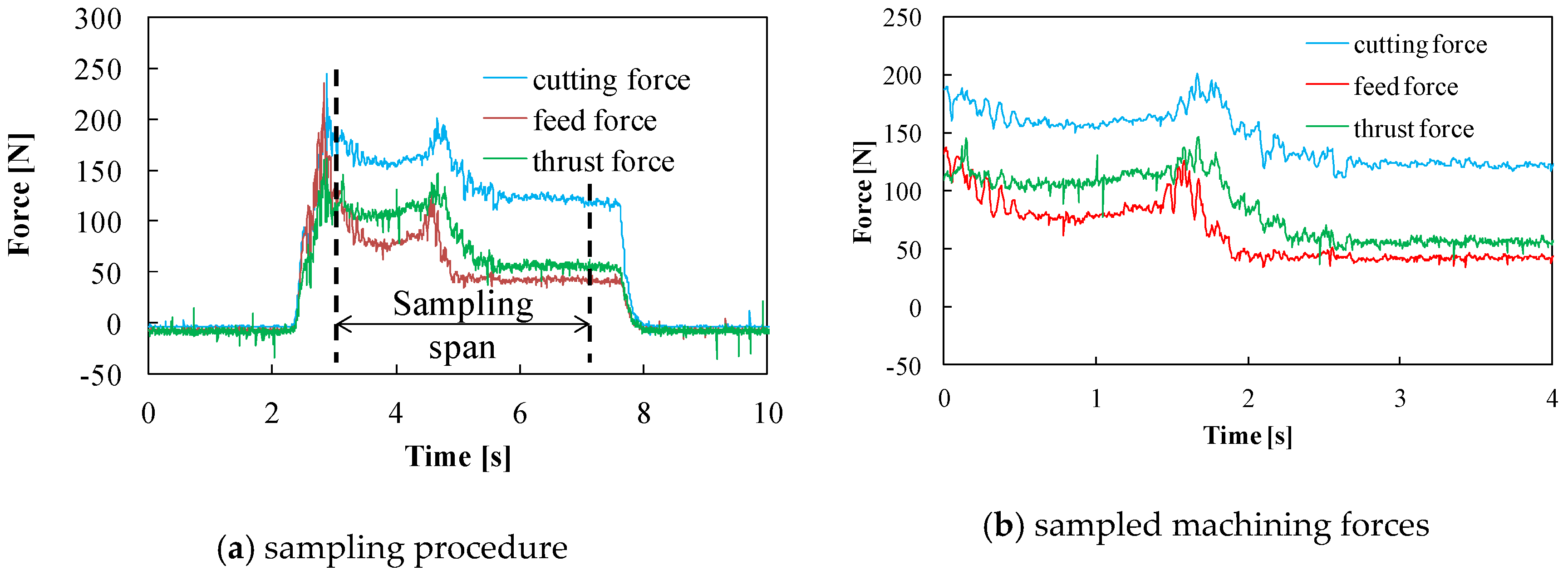
However, for the sake of analysis, the raw signals require sampling. Figure 3 schematically illustrates the sampling technique. The description is as follows. The time series of the force signals consists of the signals produced when the cutting tool approaches the cutting zone, when the cutting tool is removing materials, and when the cutting tool moves away from the cutting zone. Therefore, the raw signals, as shown in Figure 3a, require sampling. To do the sampling, a sampling span, i.e., a time interval, was chosen in such a way that the signals in the sampling span consist of cutting/feed/thrust force signals only when the cutting tool removes the materials either in the constituent material zone (i.e., in the zone of Material A and Material B) or in the joint area (i.e., the segment where Material A and B are physically connected). The case shown in Figure 3 corresponds to the sampling of the machining force signals in the joint area. The force signals after sampling were reset to a time equal to zero. Thus, the following relationships hold between the raw and sampled signals.

Let F_RX(t), t = 0, Δ, …, T1, T1 + Δ, …, T2, … be the raw signals of X, ∀X ∈ {C, F, T}. Here, C, F, and T mean cutting, feed, and thrust force signals, respectively. The interval [T1, T2] is the sampling span. The symbol Δ is the sampling interval of the raw signals F_RX(t). As mentioned before, here Δ = 0.2 ms. The segment of signals F_RX(t = T1), …, F_RX(t = T2) is used to get the sampled signals. However, the time interval in the sampled signal can be increased for the sake of analysis. Let F_SX(τ) be the sampled signals. Thus, F_SX(τ = 0) = F_RX(t = T1), F_SX(τ = λΔ) = F_RX(t = T1 + λΔ), …, F_SX(τ = nλΔ) = F_RX(t = T2). This means that the sampled signal consists of n + 1 data points, and the data points are collected using a time interval λΔ. If λ = 5, and Δ = 0.2 ms, then λΔ = 1 ms, i.e., the time interval of the sampled signal is 1 ms. Therefore, F_SX(τ) means cutting, feed, or thrust force signals at a time interval of 1 ms where X = C, F, or T, respectively. This convention is used throughout this article. The pictures of the specimens taken after machining are shown in Appendix A.

3. Analyzing Machining Forces Underlying SU–SC

This section describes the machining forces underlying the bimetallic specimens denoted as SU–SC.

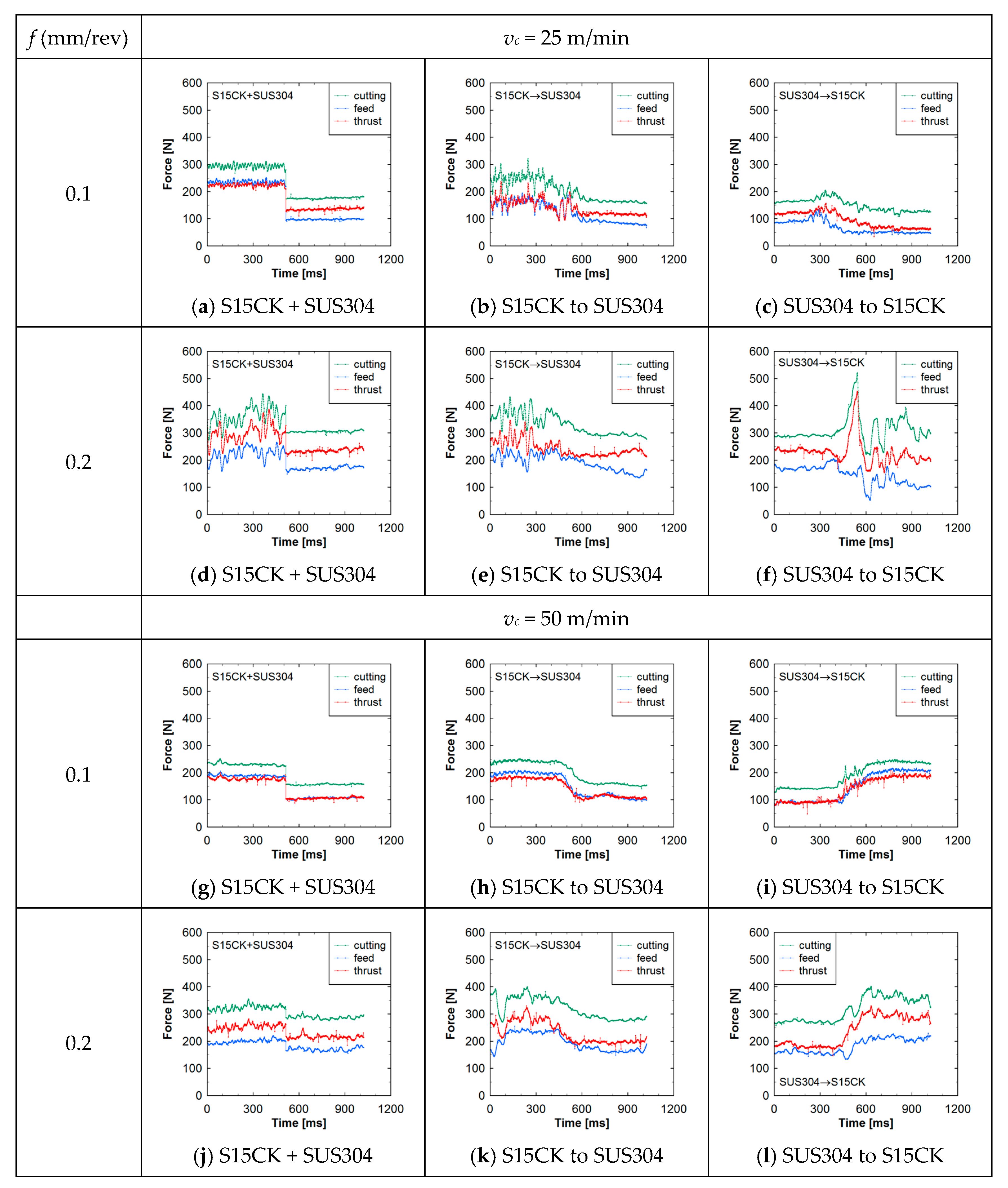
Figure 4 shows the machining forces (thrust, feed, and cutting forces) in the time domain. The plots in Figure 4a,d,g,j show the expected machining forces of the constituent materials (S15CK + SUS304), neglecting the joint area. The plots in Figure 4b,e,h,k show the machining forces manifested in the joint area while machining from the S15CK direction to the SUS304 direction. The plots in Figure 4c,f,i,l show the machining forces manifested in the joint area while machining from the SUS304 direction to the S15CK direction. As seen in Figure 4, if a low feed (0.1 mm/rev) and low cutting speed (25 m/min) are used and machining is done from the hard material (SUS304) direction to the soft material (S15CK) direction, then the machining forces can be reduced. When a high feed is preferred, then the choice is to machine from the opposite direction—from the soft material (S15CK) direction to the hard material (SUS304) direction. For a high cutting speed (50 m/min), this argument is still valid for both low and high feeds, but a low feed is perhaps a better option.

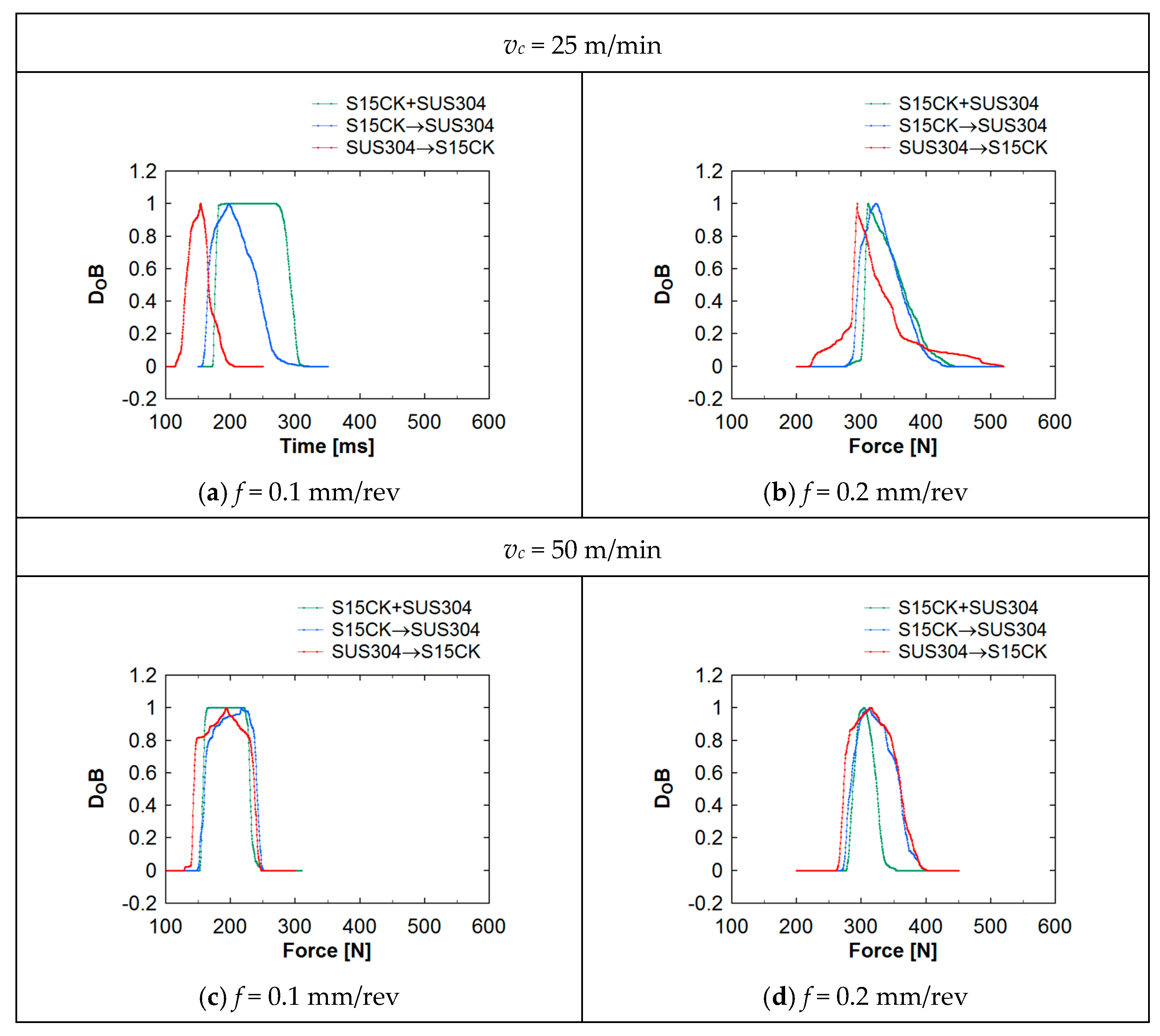
To be more specific, the uncertainty in the cutting forces was studied by constructing the possibility distributions [25,26] (probability-distribution-neutral representation of uncertainty) for the cutting forces, as shown in Figure 4. Appendix B shows the mathematical settings for inducing a possibility distribution from a set of numerical data. The results are shown in Figure 5. In the plots in Figure 5, the phrase “DoB” means the degree of belief (or membership value, see Appendix B), which is a value in the interval [0, 1]. The possibility distributions also support the abovementioned conclusions regarding the relationships between cutting conditions and cutting forces. In particular, the possibility distributions show that the use of a low feed and low cutting speed and the cutting direction hard-to-soft is a better option for reducing the cutting force and its uncertainty.

4. Analyzing Machining Forces Underlying Al–Ti

This section describes the machining forces underlying the bimetallic specimens denoted as Al–Ti. It is worth mentioning that this is a uniform combination similar to SU–SC because the tensile strength, hardness, and percent elongation of CP titanium are greater than those of aluminum (A1070), as listed in Table 1. As such, it will help validate the conclusion made in the previous section.

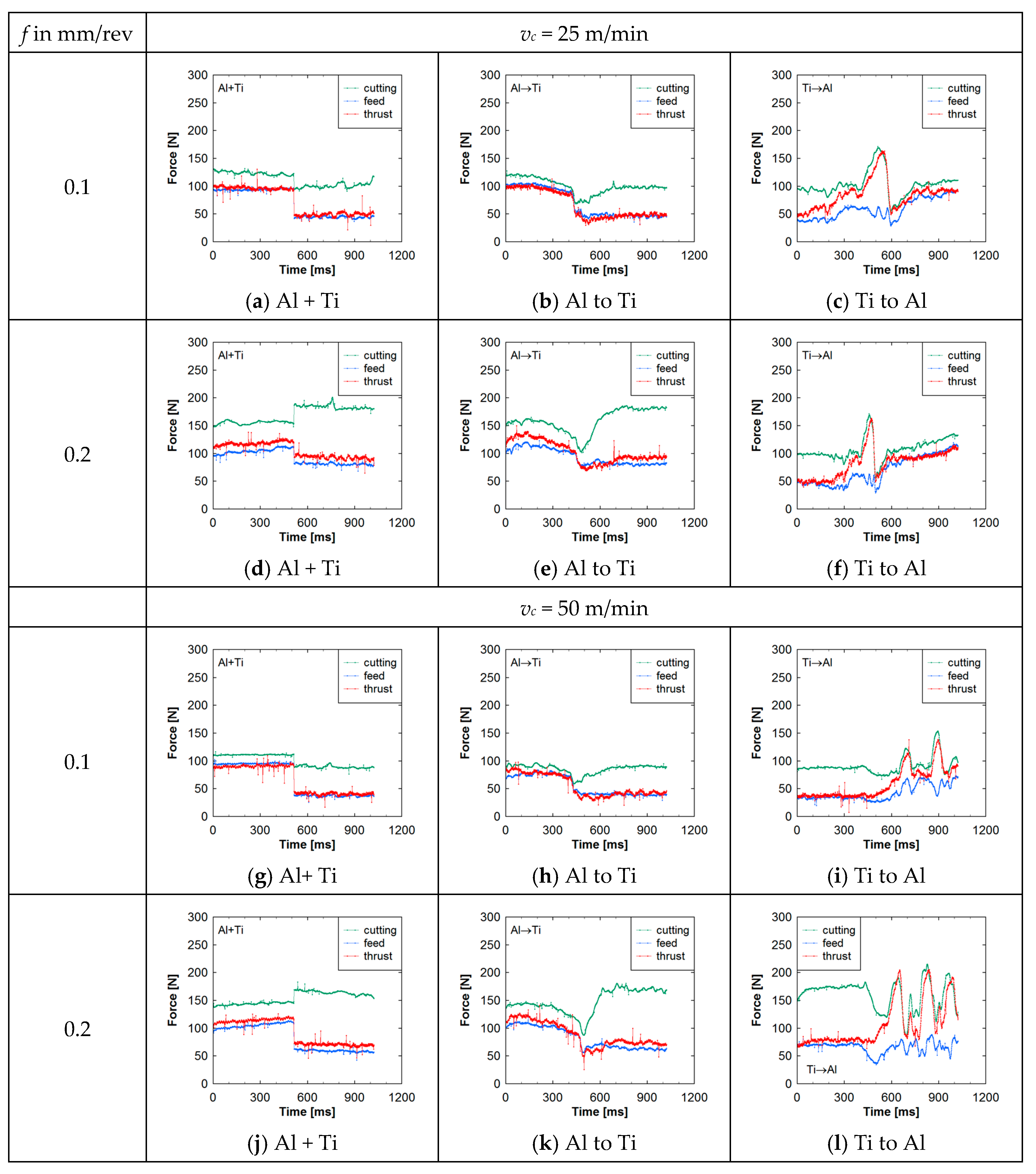
Figure 6 shows the machining forces (thrust, feed, and cutting forces) in the time domain for the dissimilar metallic specimens denoted as Al–Ti for the cutting conditions listed in Table 1. The plots in Figure 6a,d,g,j show the expected machining forces of the constituent materials (Al + Ti), neglecting the joint area. The plots in Figure 6b,e,h,k show the machining forces manifested in the joint area while machining from the Al direction to the Ti direction. The plots in Figure 6c,f,i,l show the machining forces manifested in the joint area while machining from the Ti direction to the Al direction. As seen in Figure 6, if a low feed (0.1 mm/rev) and low cutting speed (25 m/min) are used and the machining is done from the soft material (Al) direction to the hard material (Ti) direction, then the machining forces can be reduced. The same conclusion regarding the feed is valid for a high cutting speed. This is somewhat an opposing conclusion compared to that of the previous case. The reason for this somewhat dissimilar result is perhaps the hardness of the materials. Here, Al is too soft compared to the other material. This means that when a very soft metal is used in a dissimilar metallic object, it is better to start the machining operation from the soft material side using a low feed and low cutting speed.

To be more specific, the uncertainty in the cutting forces shown in Figure 6 was further studied by constructing possibility distributions similar to the previous case. The results are shown in Figure 7. The possibility distributions also support the abovementioned conclusions regarding the relationships between cutting conditions and cutting forces. In particular, the possibility distribution shows that the use of a low feed and low cutting speed and employing the cutting direction soft-to-hard is the right approach for reducing the cutting force and its uncertainty.

5. Analyzing Machining Forces Underlying Al–CI

This section describes the machining forces underlying the bimetallic specimens denoted as Al–CI. It is worth mentioning that this is a uniform combination similar to the previous two cases, because the tensile strength, hardness, and percent elongation of cast iron are greater than those of aluminum (A5052), as listed in Table 1 (note that the hardness equal to 79.2 HRB is about 142 HV.) Compared to the previous case, the Al alloy used here is much harder. As such, it will help validate the conclusions made in the previous two sections.

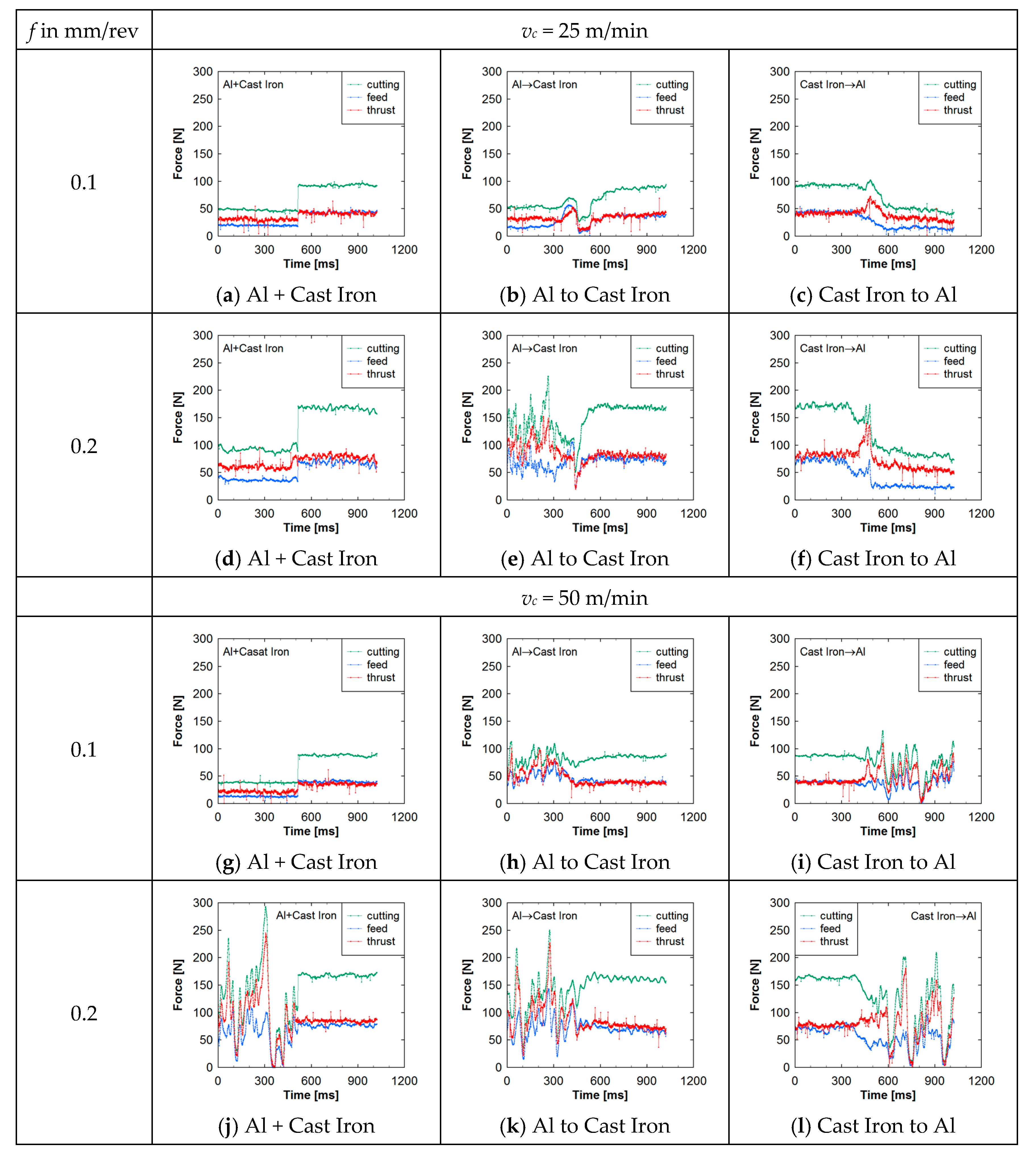
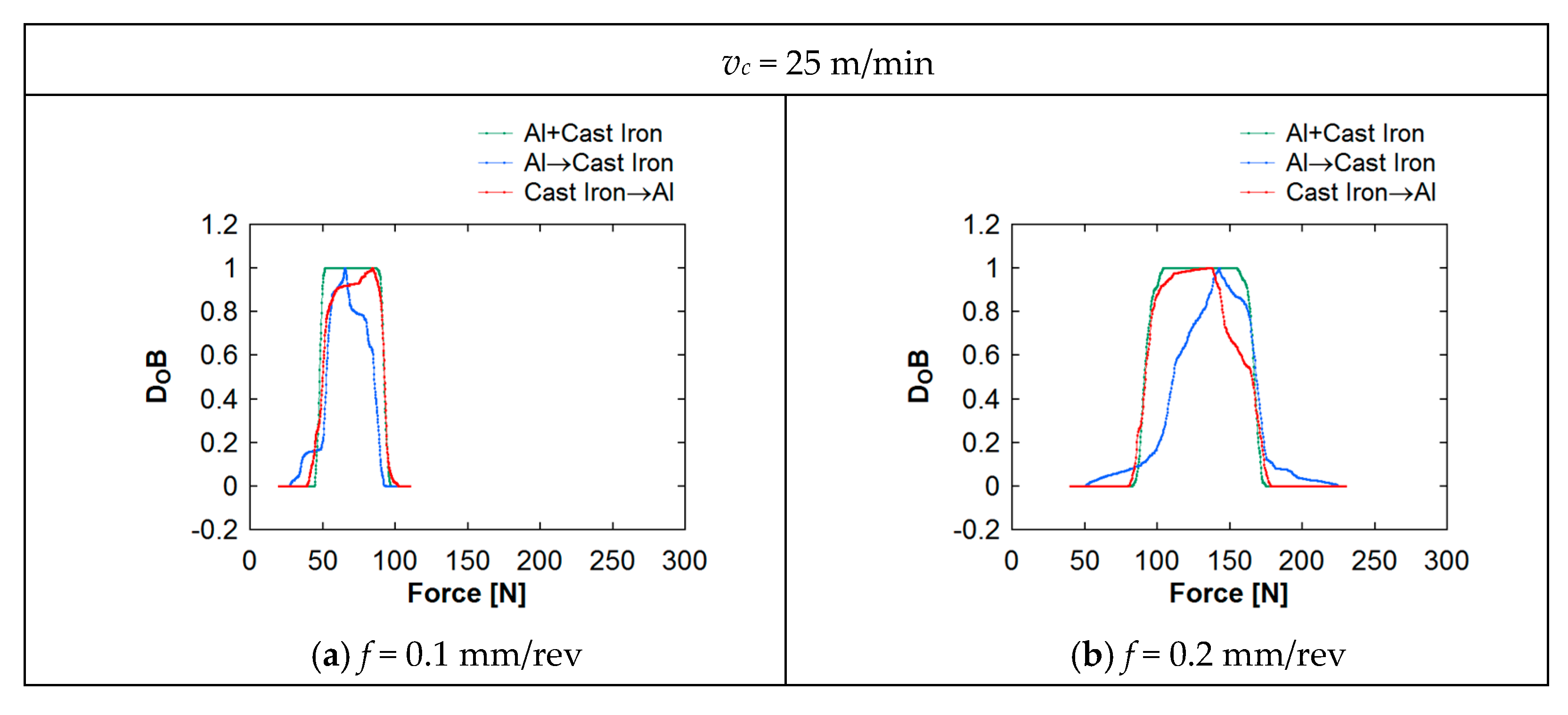
Figure 8 shows the machining forces (thrust, feed, and cutting forces) in the time domain for the dissimilar metallic specimens denoted as Al–CI for the cutting conditions listed in Table 1. The plots in Figure 8a,d,g,j show the expected machining forces of the constituent materials (Al + CI), neglecting the joint area. The plots in Figure 8b,e,h,k show the machining forces manifested in the joint area while machining from the Al direction to the CI direction. The plots in Figure 8c,f,i,l show the machining forces manifested in the joint area while machining from the CI direction to the Al direction. As seen in Figure 8, if a low feed (0.1 mm/rev) and low cutting speed (25 m/min) are used, both machining directions provide similar cutting forces. For the high cutting speed, the machining direction soft-to-hard provides a better result only for the low feed. To be more specific, the uncertainty in the cutting forces shown in Figure 8 was further studied by constructing the possibility distributions similar to the previous two cases. The results are shown in Figure 9. The possibility distributions also support the abovementioned conclusions regarding the relationships between cutting conditions and cutting forces. In particular, the possibility distributions show that the use of a low feed and low cutting speed and using the cutting direction soft-to-hard is the best procedure for reducing the cutting force and its uncertainty.

6. Discussions

Manufacturers who support sustainable product development (including design, manufacturing, and assembly) can benefit from the outcomes of this study because parts/products made of dissimilar materials (or multi-material objects) are better than their mono-material counterparts in terms of sustainability (cost, weight, and CO₂ footprint). Particularly, this kind of study will help them by supplying the knowledge of material wastages and energy conceptions during the manufacturing processes. Regarding the material wastage calculation, the methodology described in [2] can be used. As far as the energy consumption is concerned, the machining force signals shown in Figure 4, Figure 5, Figure 6, Figure 7, Figure 8 and Figure 9 can be used. For example, the machining power (P_M) (kW) can be estimated using the cutting and feed force signals, which is a useful piece of information for determining the energy efficiency of a manufacturing process [2]. The machining power, denoted as P_M, has two components, namely, Cutting power (P_c) and Feed power (P_f) components. As such, the following formulation holds:

P_{M} (i) = P_{c} (i) + P_{f} (i) = \frac{1}{60 \times 10^{3}} [F_{S C} (i) v_{c} + \frac{F_{S F} (i) f N}{10^{3}}]

(1)

Figure 10 shows, for example, the P_M of the bimetallic specimen called SU–SC for the cutting conditions v_c = 25 m/min and f = 0.2 mm/rev. As seen in Figure 10, P_M varies in the range of [0.2, 0.45] kW. The variability in the cutting power for the four possibilities are illustrated in Figure 10a–d that correspond to the segments S15CK, SUS304, S15CK to SUS304, and SUS304 to S15CK, respectively. When the cutting tool passes the joint area, a gradual decrease/increase in the cutting power is observed, which is similar to that of the machining forces. This means that when the force sensors are not available, a power measurement instrument can be used to monitor the machining behavior of a bimetallic object.

7. Concluding Remarks

This study reports the cutting/feed/thrust forces exhibited by three sets of bimetallic specimens. It was found that an entirely different machining force behavior arises due to the presence of two different materials, as well as the joint area.

The results shown in Figure 4, Figure 5, Figure 6, Figure 7, Figure 8 and Figure 9 lead to the following conclusions:

Referring to the results in Figure 4 and Figure 5, while machining steel-based bimetallic objects, keeping a low feed and high cutting speed is the better option, and the machining operation can be performed in both hard-to-soft and soft-to-hard material directions, but machining in the soft-to-hard material direction is the better option.

It is not recommended to create a bimetallic object using very soft material. Otherwise, it creates a machining problem (e.g., the case shown in Figure 6 and Figure 7).

If an aluminum-based bimetallic part is preferred, then it is better to use a relatively harder alloy (e.g., compare the results shown in Figure 6 and Figure 7 with those of shown in Figure 8 and Figure 9). For the aluminum-based bimetallic objects, it is better to machine at a low cutting speed and low feed when the hard-to-soft material direction is needed.

Nevertheless, the research on machining is mostly concerned with the machining of objects made of mono-material and special alloys, whereas the research on machining objects made of multiple materials is in its infancy. The outcomes of this study can be used as a reference while enriching the machining technology of multi-material parts.

Funding

This work was funded by Kitami Institute of Technology.

Acknowledgments

The author gratefully acknowledges two of his former graduate students, Shin Matsui and Dongyuan Wu, and Masaaki Kimura at the University of Hyogo for their valuable inputs during the course of this study.

Conflicts of Interest

The author declares no conflict of interest.

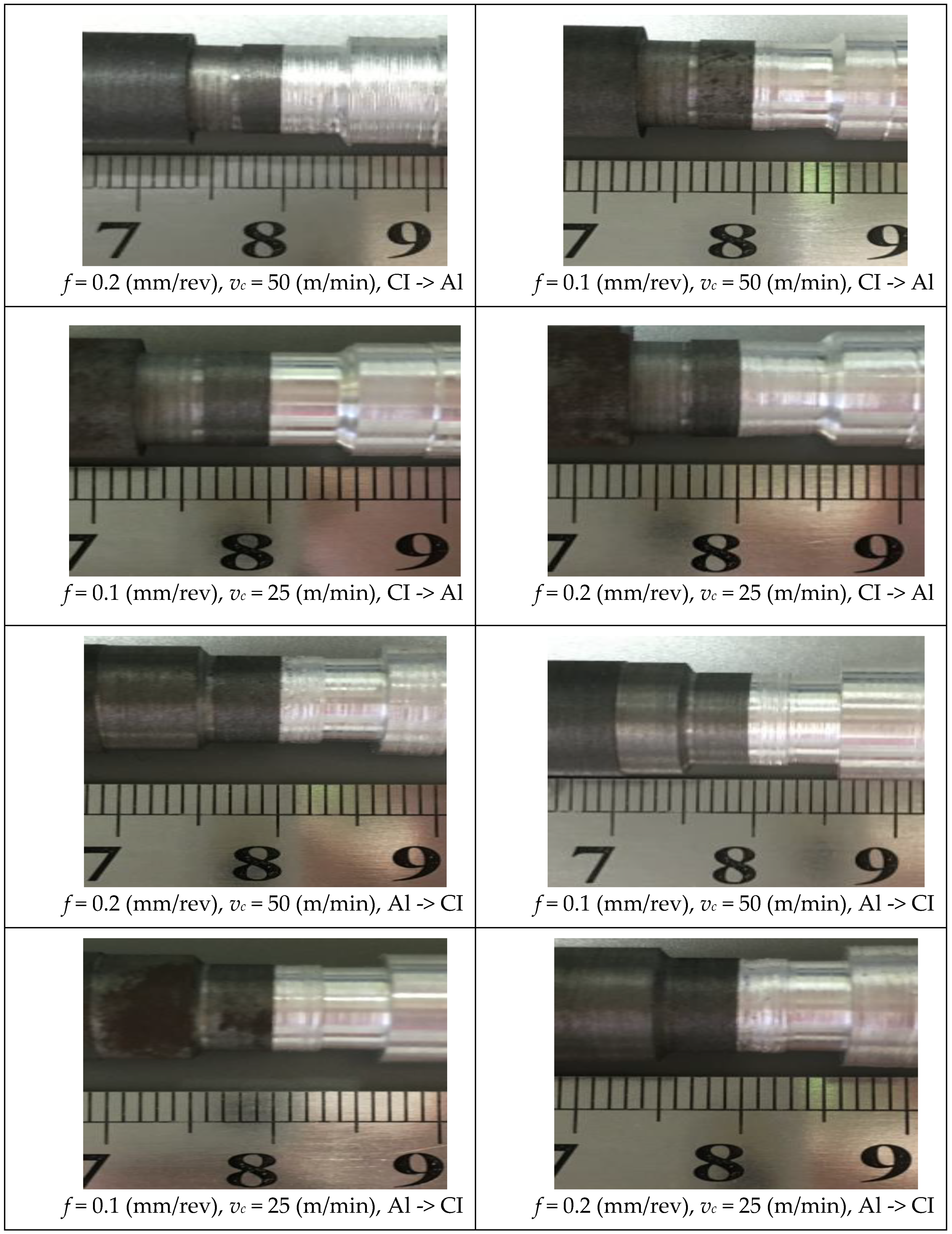
Appendix A. Pictures of the Bimetallic Specimens Taken after Machining

This Appendix shows the pictures of the three types of specimens after conducting the turning experiments. The respective cutting conditions and directions are shown.

Figure A1. The SU–SC specimens.

Figure A2. The Al–Ti specimens.

Figure A3. The Al–CI specimens.

Appendix B. Inducing Possibility Distributions (Fuzzy Numbers) from Numerical Data

This appendix describes the mathematical procedures used to induce the possibility distributions (fuzzy numbers) from the time series of machining forces. The same procedure can be found in [25,26].

Let x(t) ∈ ℜ, t = 0, …, n − 1 be n data points in the form of a time series, as shown in Figure A4.

Figure A4. A given set of numerical data.

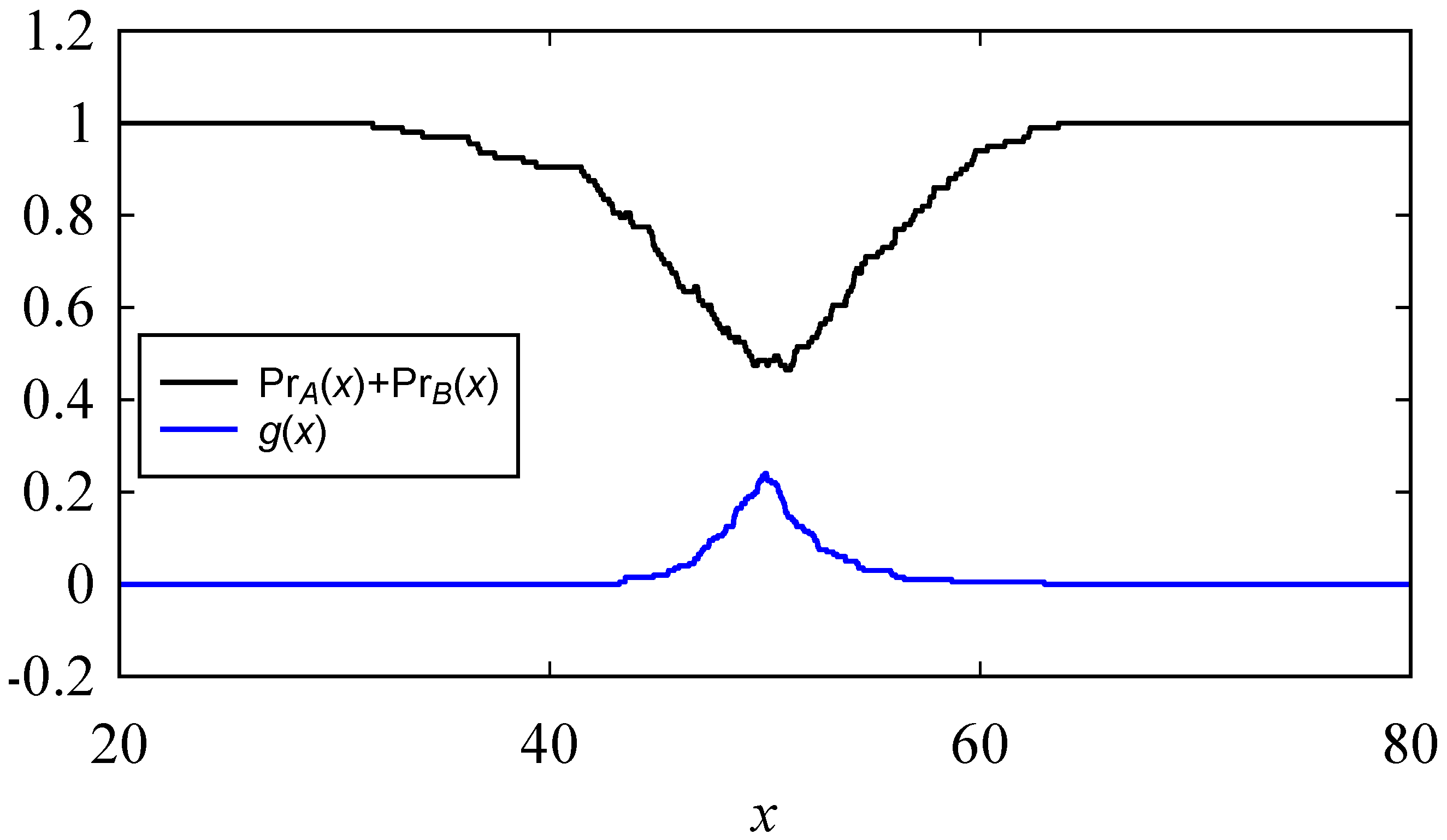
Let (x(t), x(t + 1)), t = 0, …, n − 1 be a point-cloud in the universe of discourse X = [x_min, x_max] so that x_min < min(x(t)| ∀t ∈ {0, …, n}) and x_max > max(x(t)| ∀t ∈ {0, …, n}). Let A and B two square boundaries so that the vectors of the vertices of A and B (in the anti-clockwise direction) are ((x_min, x_min), (x, x_min), (x, x), (x_min, x)) and ((x_max, x_max), (x, x_max), (x, x), (x_max, x)), respectively, ∀x ∈ X. As such, (x, x) is the common vertex of A and B. For example, consider the arbitrary point-cloud shown in Figure A5. According to Figure A5, the universe of discourse is as follows, X = [20, 80]. Notice the relative positions of the boxes denoted as A and B in Figure A5. The boxes are connected at their common vertices.

Figure A5. Relative position of A and B in the point-cloud (x(t), x(t + 1)).

Let Pr_A(x) and Pr_B(x) be two subjective probabilities, wherein Pr_A(x) and Pr_B(x) represent the degrees of chance that the points in the point-cloud are in A and B, respectively. As such, these functions are defined by the following mappings:

\begin{array}{l} X \to [0, 1] \\ x \mapsto \Pr_{A} (x) = \frac{\sum_{i = 0}^{n - 1} Θ (t)}{n - 1} \\ Θ (t) = {\begin{cases} 1 ((x (t) \leq x) \land (x (t + 1) \leq x)) \\ 0 o t h e r w i s e \end{cases} \end{array}

(A1)

\begin{array}{l} X \to [0, 1] \\ x \mapsto \Pr_{B} (x) = \frac{\sum_{i = 0}^{n - 1} Ω (t)}{n - 1} \\ Ω (t) = {\begin{cases} 1 ((x (t) \geq x) \land (x (t + 1) \geq x)) \\ 0 o t h e r w i s e \end{cases} \end{array}

(A2)

The typical natures of the functions defined in Equations (A1) and (A2) are illustrated in Figure A6, using the information of the point-cloud shown in Figure A5. Note that Pr_A(x) increases with the increase in x, and the opposite is true for Pr_B(x). It is worth mentioning that Pr_A(x) + Pr_B(x) ≤ 1 for the point-cloud, though for some cases, Pr_A(x) + Pr_B(x) = 1 (see Figure A7). This means that the expression Pr_A(x) + Pr_B(x) does not serve the role of “cumulative probability distribution.” A cumulative probability distribution can, however, be formulated by using the information of Pr_A(x) and Pr_B(x), as shown in Figure A7.

Figure A6. The typical nature of Pr_A(x) and Pr_B(x) for unimodal quantity.

Figure A7. Nature of Pr_A(x) + Pr_B(x) and min(Pr_A(x), Pr_B(x)) for unimodal data.

Consider a mapping that maps x into the minimum of Pr_A(x) and Pr_B(x), as follows:

\begin{array}{l} X \to [0, a] \\ x \mapsto g (x) = \min (\Pr_{A} (x), \Pr_{B} (x)) \end{array}

(A3)

In Equation (A3), a = 1 if the point-cloud is a point; otherwise, a < 1. Figure A7 shows the nature of g(x) with respect to Pr_A(x) + Pr_B(x). The area under g(x) is given by:

Q = \int_{X} g (x) d x

(A4)

There is no guarantee that Q = 1. Otherwise, g(x) could have been considered a probability distribution of the underlying point-cloud. However, a function F(x) can be defined as follows:

\begin{array}{l} [0, a] \to [0, 1] \\ x \mapsto F (x) = \frac{\int_{x_{\min}}^{x} g (x) d x}{Q} \end{array}

(A5)

F(x) can be considered a cumulative probability distribution because max(F(x)) = 1, F(x) ≥ F(z) for x ≥ z, F(x) ∈ [0, 1], ∀x, z ∈ X. Figure A8 shows the nature of F(x) derived from g(x) shown in Figure A7. The cumulative probability distribution defined in Equation (A5) produces a probability distribution Pr(x). Thus, the following formulation holds:

\Pr (x) = \frac{d F (x)}{d x}

(A6)

Figure A9 shows the probability distribution Pr(x) that corresponds to F(x) as shown in Figure A8. The area under the probability distribution Pr(x) is unit and Pr(x) remains in the bound of [0, 1].

From the induced probability distribution Pr(x), a possibility distribution given by the membership function μ_I(x)) can be defined based on the heuristic rule of probability-possibility transformation—the degree of possibility is greater than or equal to the degree of probability. The easiest formulation is to normalize Pr(x) by its maximum value, max(Pr(x) | ∀x ∈ X), yielding the following formulation:

\begin{array}{l} [0, 1] \to [0, 1] \\ \Pr (x) \mapsto μ_{I} (x) = \frac{\Pr (x)}{\max (\Pr (x) | \forall x \in X)} \end{array}

(A7)

Figure A10 shows the possibility distribution μ_I(x) derived from the probability distribution Pr(x) shown in Figure A9. The shape of the induced probability and possibility distributions are identical, as evident from Figure A9 and Figure A10, respectively. Other formulations can be used instead of the formulation (A7), if needed.

Figure A8. Nature of cumulative probability distribution of a point-cloud.

Figure A9. The nature of the probability distribution of a unimodal point-cloud.

Figure A10. The nature of the possibility distribution of a unimodal point-cloud.

However, it is observed that when the point-cloud resembles the point-cloud of a bimodal quantity, the induced possibility distribution resembles a trapezoidal fuzzy number. In addition, when the point-cloud is a point, the induced possibility distribution becomes a fuzzy singleton. Moreover, when the point-cloud resembles the point-cloud of unimodal data, the induced probability/possibility distribution resembles a triangular fuzzy number. To define the membership function of an induced fuzzy number in the form of a triangular fuzzy number, the following formulation can be used.

Let u, v, and w be three points in ascending order in the universe of discourse X, u ≤ v ≤ w ∈ X. Let the interval [u, w] be the support of a triangular fuzzy number and the point v be the core. The following procedure can be used to determine the values of u, v, and w from the induced fuzzy number μ_I(x) (Equation (A7)):

\begin{array}{l} u \leq v \leq w \in X \\ u = x (μ_{I} (x) = 0 \land μ_{I} (x + d x) > 0) \\ v = x (μ_{I} (x - d x) < 1 \land μ_{I} (x) = 1) \\ w = x (μ_{I} (x - d x) > 0 \land μ_{I} (x) = 0) \end{array}

(A8)

As defined in (A8), u is the point after which the membership value μ_I(x) is greater than zero, v is the point corresponding to the maximum membership value max(μ_I(x)), and w is the point from/beyond which the membership value μ_I(x) again becomes/remains zero. Thus, the membership function of the induced triangular fuzzy number denoted as μ_T(x) is as follows:

\begin{array}{l} X \to [0, 1] \\ x \mapsto μ_{T} (x) = \max (0, \min (\frac{x - u}{v - u}, \frac{w - x}{w - v})) \end{array}

(A9)

In this article, the formulations up to (A7) were used, i.e., the regular fuzzy number was not constructed. The triangular fuzzy numbers are particularly important when the optimization of cutting conditions is carried out using the experimental data obtained by using a statistical procedure (e.g., design of experiment), as shown in [26].

References

United Nations Environment Program. Report of the World Commission on Environment and Development Annex to General Assembly Document a/42/427; United Nations: Nairobi, NY, USA, 1987. [Google Scholar]
Ullah, A.M.M.S.; Fuji, A.; Kubo, A.; Tamaki, J. Analyzing the sustainability of bimetallic components. Int. J. Autom. Technol. 2014, 8, 745–753. [Google Scholar] [CrossRef]
Allwood, J.M.; Ashby, M.F.; Gutowski, T.G.; Worrell, E. Material efficiency: A white paper. Resour. Conserv. Recycl. 2011, 55, 362–381. [Google Scholar] [CrossRef]
Bian, J.; Mohrbacher, H.; Zhang, J.-S.; Zhao, Y.-T.; Lu, H.-Z.; Dong, H. Application potential of high performance steels for weight reduction and efficiency increase in commercial vehicles. Adv. Manuf. 2015, 3, 27–36. [Google Scholar] [CrossRef] [Green Version]
Ullah, A.M.M.S.; Hashimoto, H.; Kubo, A.; Tamaki, J. Sustainability analysis of rapid prototyping: Material/resource and process perspectives. Int. J. Sustain. Manuf. 2013, 3, 20–36. [Google Scholar] [CrossRef]
Kimura, M.; Kusaka, M.; Kaizu, K.; Fuji, A. Effect of post-weld heat treatment on joint properties of friction welded joint between brass and low carbon steel. Sci. Technol. Weld. Join. 2010, 15, 590–596. [Google Scholar] [CrossRef]
Kimura, M.; Fuji, A.; Konno, Y.; Itoh, S.; Kim, Y.C. Investigation of fracture for friction welded joint between pure nickel and pure aluminium with post-weld heat treatment. Mater. Des. 2014, 57, 503–509. [Google Scholar] [CrossRef]
Sahu, P.K.; Kumari, K.; Pal, S.; Pal, S.K. Hybrid fuzzy-grey-Taguchi based multi weld quality optimization of Al/Cu dissimilar friction stir welded joints. Adv. Manuf. 2016, 4, 237–247. [Google Scholar] [CrossRef]
Buffa, G.; de Lisi, M.; Sciortino, E.; Fratini, L. Dissimilar titanium/aluminum friction stir welding lap joints by experiments and numerical simulation. Adv. Manuf. 2016, 4, 287–295. [Google Scholar] [CrossRef]
Gibson, I.; Rosen, D.; Stucker, B. Additive Manufacturing Technologies: 3D Printing, Rapid Prototyping, and Direct Digital Manufacturing, 2nd ed.; Springer: New York, NY, USA, 2015. [Google Scholar]
Bourell, D.L.; Rosen, D.W.; Leu, M.C. The Roadmap for Additive Manufacturing and Its Impact. Print. Addit. Manuf. 2016, 1, 231–238. [Google Scholar] [CrossRef]
Ullah, A.M.M.S. Design for additive manufacturing of porous structures using stochastic point-cloud: A pragmatic approach. Comput. Aided Des. Appl. 2018, 15, 138–146. [Google Scholar] [CrossRef]
Tateno, T. Anisotropic Stiffness Design for Mechanical Parts Fabricated by Multi-Material Additive Manufacturing. Int. J. Autom. Technol. 2016, 10, 231–238. [Google Scholar] [CrossRef]
Song, X.; Lieh, J.; Yen, D. Application of small-hole dry drilling in bimetal part. J. Mater. Process. Technol. 2007, 186, 304–310. [Google Scholar] [CrossRef]
Uthayakumar, M.; Prabhaharan, G.; Aravindan, S.; Sivaprasad, J.V. Machining studies on bimetallic pistons with CBN tool using the Taguchi method—Technical communication. Mach. Sci. Technol. 2008, 12, 249–255. [Google Scholar] [CrossRef]
Uthayakumar, M.; Prabhakaran, G.; Aravindan, S.; Sivaprasad, J.V. Influence of Cutting Force on Bimetallic Piston Machining by a Cubic Boron Nitride (CBN) Tool. Mater. Manuf. Process. 2012, 27, 1078–1083. [Google Scholar] [CrossRef]
Manikandan, G.; Uthayakumar, M.; Aravindan, S. Machining and simulation studies of bimetallic pistons. Int. J. Adv. Manuf. Technol. 2013, 66, 711–720. [Google Scholar] [CrossRef]
Malakizadi, I.; Sadik, L. Nyborg, Wear Mechanism of CBN Inserts During Machining of Bimetal Aluminum-grey Cast Iron Engine Block. Procedia CIRP 2013, 8, 188–193. [Google Scholar] [CrossRef]
Ullah, A.M.M.S.; Fuji, A.; Kubo, A.; Tamaki, J.; Kimura, M. On the Surface Metrology of Bimetallic Components. Mach. Sci. Technol. 2015, 19, 339–359. [Google Scholar] [CrossRef]
Matsui, S.; Ullah, S.; Kubo, A.; Fuji, A. Cutting force signal processing for machining bimetallic components. In Proceedings of the International Conference on Leading Edge Manufacturing in 21st Century: LEM21, Tokyo, Japan, 18–22 October 2015. [Google Scholar] [CrossRef]
Wu, D.; Ullah, S.; Kubo, A.; Fuji, A. On the complexity in roughness quantification across bimetallic boundary. In Proceedings of the International Conference on Leading Edge Manufacturing in 21st Century: LEM21, Tokyo, Japan, 18–22 October 2015. [Google Scholar] [CrossRef]
Kaynak, Y.; Kitay, O. Porosity, Surface Quality, Microhardness and Microstructure of Selective Laser Melted 316L Stainless Steel Resulting from Finish Machining. J. Manuf. Mater. Process. 2018, 2, 36. [Google Scholar] [CrossRef]
Cabrera, C.G.; Araujo, A.C.; Castello, D.A. On the wavelet analysis of cutting forces for chatter identification in milling. Adv. Manuf. 2017, 5, 130–142. [Google Scholar] [CrossRef]
Ullah, A.M.M.S.; Akamatsu, T.; Furuno, M.; Chowdhury, M.A.K.; Kubo, A. Strategies for Developing Milling Tools from the Viewpoint of Sustainable Manufacturing. Int. J. Autom. Technol. 2016, 10, 727–736. [Google Scholar] [CrossRef]
Ullah, A.M.M.S.; Shamsuzzaman, M. Fuzzy Monte Carlo Simulation using point-cloud-based probability–possibility transformation. Simulation 2013, 89, 860–875. [Google Scholar] [CrossRef]
Chowdhury, M.A.K.; Sharif Ullah, A.M.M.; Anwar, S. Drilling High Precision Holes in Ti6Al4V Using Rotary Ultrasonic Machining and Uncertainties Underlying Cutting Force, Tool Wear, and Production Inaccuracies. Materials 2017, 10, 1069. [Google Scholar] [CrossRef] [PubMed]

Figure 1. The pictures of the bimetallic specimens.

Figure 2. Experimental setup.

Figure 3. Force data after sampling.

Figure 4. Machining forces underlying SU–SC.

Figure 5. Uncertainties in the machining forces underlying SU–SC.

Figure 6. Machining forces underlying Al–Ti.

Figure 7. Uncertainties in the machining forces underlying Al–Ti.

Figure 8. Machining forces underlying Al–CI.

Figure 9. Uncertainties in the machining forces underlying Al–CI.

Figure 10. Machining power of the SU–SC bimetallic specimen (v_c = 25 m/min, f = 0.2 mm/rev).

Table 1. Materials used for fabricating the dissimilar metallic specimens.

Bimetallic Specimens	Materials	Tensile Strength	Elongation	Hardness
Bimetallic Specimens	Materials	(MPa)	(%)	(Scale)
SU–SC	Stainless Steel	663	55	182
	(JIS: SUS304)	663	55	(HV)
	Mild Steel	439	38	132
	(JIS: S15CK)	439	38	(HV)
Al–Ti	Aluminum	120	27	41
	(JIS: A1070)	120	27	(HV)
	Commercial Pure (CP) Titanium	401	35	146
	Commercial Pure (CP) Titanium	401	35	(HV)
Al–CI	Aluminum	265	17.4	86
	(JIS: A5052)	265	17.4	(HV)
	Ductile Cast Iron	442	18.6	79.2
	Ductile Cast Iron	442	18.6	(HRB)

Table 2. Friction welding conditions for fabricating the dissimilar metallic specimens.

Friction Welding Conditions	Specimens
Friction Welding Conditions	SU-SC	Al-Ti	Al-CI
Rotating material	S15CK	A1070	A5052
Diameter of the rotating material (mm)	12
Friction speed (s⁻¹)	27.5 (1650 rpm)
Friction pressure (MPa)	30
Friction time (s)	2	1	3
Upset pressure (MPa)	270	90	200
Upset time (s)	6

Table 3. Cutting conditions for machining experiments.

Items	Descriptions
Machine Tool	Lathe Machine Make: WASHINO Model: LEO-80A
Cutting Tool	Carbide CVD Coated Insert Make: Sandvik™ Code: TNMG160404-MF
Cutting Speed (v_c) (m/min)	25, 50
Rotational Speeds of the Chuck (rpm)	1377
Feed (f) (mm/rev)	0.1, 0.2
Depth of Cut (a_p) (mm)	1
Cutting Direction	A to B, B to A (for the joint area)

© 2018 by the author. Licensee MDPI, Basel, Switzerland. This article is an open access article distributed under the terms and conditions of the Creative Commons Attribution (CC BY) license (http://creativecommons.org/licenses/by/4.0/).

Share and Cite

MDPI and ACS Style

Ullah, A.S. Machining Forces Due to Turning of Bimetallic Objects Made of Aluminum, Titanium, Cast Iron, and Mild/Stainless Steel. J. Manuf. Mater. Process. 2018, 2, 68. https://doi.org/10.3390/jmmp2040068

AMA Style

Ullah AS. Machining Forces Due to Turning of Bimetallic Objects Made of Aluminum, Titanium, Cast Iron, and Mild/Stainless Steel. Journal of Manufacturing and Materials Processing. 2018; 2(4):68. https://doi.org/10.3390/jmmp2040068

Chicago/Turabian Style

Ullah, AMM Sharif. 2018. "Machining Forces Due to Turning of Bimetallic Objects Made of Aluminum, Titanium, Cast Iron, and Mild/Stainless Steel" Journal of Manufacturing and Materials Processing 2, no. 4: 68. https://doi.org/10.3390/jmmp2040068

Article Menu

Machining Forces Due to Turning of Bimetallic Objects Made of Aluminum, Titanium, Cast Iron, and Mild/Stainless Steel

Abstract

1. Introduction

2. Machining Experiments and Data Acquisition

3. Analyzing Machining Forces Underlying SU–SC

4. Analyzing Machining Forces Underlying Al–Ti

5. Analyzing Machining Forces Underlying Al–CI

6. Discussions

7. Concluding Remarks

Funding

Acknowledgments

Conflicts of Interest

Appendix A. Pictures of the Bimetallic Specimens Taken after Machining

Appendix B. Inducing Possibility Distributions (Fuzzy Numbers) from Numerical Data

References

Share and Cite

Article Metrics

Article Access Statistics

Further Information

Guidelines

MDPI Initiatives

Follow MDPI